Estimating Volume Loss for Shield-Driven Tunnels Based on the Principle of Minimum Total Potential Energy

Abstract

Volume loss is an important method to estimate ground movement during tunnelling. However, volume loss is usually estimated by empirical methods, especially for volume loss at the tunnel face, which is a three-dimensional problem. Based on the principle of minimum total potential energy, we proposed a semi-analytical method to predict the volume loss at the tunnel face and ground surface. The proposed method provides a more direct way of estimating volume loss at the tunnel face from an energy point of view. Moreover, a new deformation mechanism was designed to describe the ground movement before the tunnel face. Based on the proposed method, we investigated the influence of the support pressure, tunnel diameter, and tunnel depth on the volume loss at the tunnel face, and other parameters related to surface subsidence. The volume loss at the tunnel face decreased with the increase in the support pressure ratio and the slurry weight. The volume loss at ground surface was generally smaller than the volume loss at the tunnel face due to the soil compression during ground movement. The bigger the tunnel diameter, the bigger the volume loss at the tunnel face. However, the volume loss at ground surface may not increase with the increase in tunnel depth, because of the soil arching effect. Moreover, the deeper the tunnel, the more obvious the influence of the support pressure ratio on volume loss. Similarly, the bigger the tunnel diameter, the more obvious the influence of the slurry weight on the volume loss.

1. Introduction

The slurry pressure balance shield tunnel is widely adopted in practice, and ground movement is inevitably induced during tunnel excavation. The induced ground movement may cause serious damage to existing buildings and subterranean facilities. Therefore, the estimation of ground movement is important in the design stage of tunnelling. Many researchers have contributed to analyzing the ground movement by different methods. Those methods can be divided into three categories: the analytical method [1,2,3,4,5,6,7,8], the empirical method [9,10,11], and numerical simulation [12,13,14].

Volume loss plays an important role in the analysis of ground movement. The effect of the tail grout on the volume loss was studied [15]. Different ways for determining the volume loss are summarized [11]. Furthermore, many researchers have investigated the volume loss in two-dimensional problems by assuming a zero-volume change in soil (i.e., undrained volume loss). The undrained volume loss is equal to ground loss, which is defined as the ratio of shrinkage deformation to the area of the tunnel (sometimes the undrained volume loss is called “ground loss”, in some literature). The analytical solution for the tunnel excavation as the function of the ground loss and the tunnel ovalization parameter are developed [16]. The deformation was divided into the ground loss, ovalization, and vertical movement [17]. A lot of researchers have investigated undrained volume loss with gap parameters, which was developed by considering the 3D elastoplastic deformation at the tunnel face [18]. The procedure for estimating the gap parameter was supported with 14 case monitoring data [19]. Loganathan and Poulos [3] incorporated the gap parameter into the closed-form solution derived by Verruijt and Booker [16]. Based on the work performed by Loganathan and Poulos [3], A solution for predicting the ground movement in multi-layered clayed soil was proposed [20]. The above research assumed a plane strain condition, which was limited to a two-dimension solution.

Some researchers have devoted their study to investigating the ground deformation and volume loss before the tunnel face. Based on the field monitoring data, Different relationships between the stability number, which is used in the stability analysis for tunnelling, and the volume loss before the tunnel face are established [21,22,23,24].

In recent years, the energy method has been developed rapidly in the analysis of ground deformation due to tunnelling. The two-dimensional ground movement was predicted with the balance between energy and work, ignoring soil volume change [25]. Based on the principle of energy conservation, an innovative method to predict the two-dimensional undrained volume loss were proposed [26]. Plamer and Mair [27] gave a solution for estimating volume loss in the elastic ground on the basis of the reciprocal theorem. As for volume loss at the tunnel face, Klar and Klein [28] estimated the face ‘take’ undrained volume loss with the use of a mobilizable strength design (MSD).

In this paper, we develop a method to predict volume loss at the tunnel face based on the principle of minimum total potential energy. Moreover, a new deformation mechanism is created based on a proposed deformation mechanism [29] to consider the soil volume change. Finally, we analyze the influence of support pressure supplied by slurry, tunnel diameter, and tunnel depth on volume loss. The proposed method provides a more direct way of estimating volume loss at the tunnel face from the energy point of view. The soil volume changes during ground movement are considered in the proposed method.

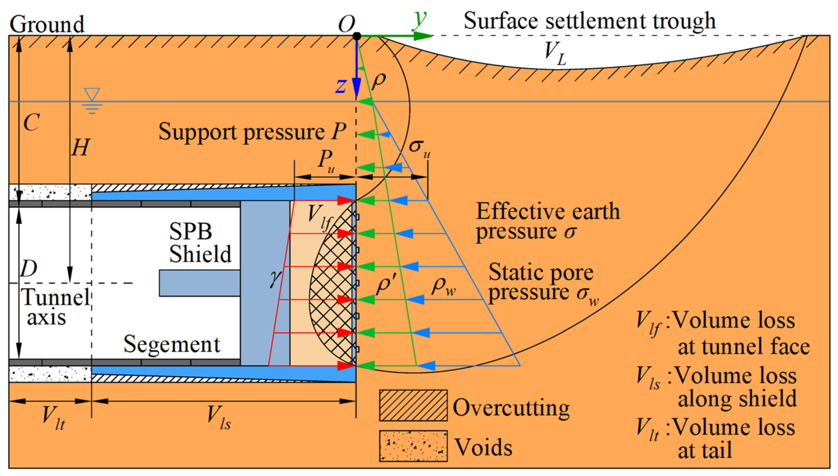
2. Problem Description

According to the causes of volume loss in slurry pressure balance shield tunnelling [10,24,30], volume loss can be categorized into three components, as shown in Figure 1:

V_lf: Volume loss at the tunnel face. The stability of the working face is achieved by the support pressure provided by a pressurized mixture of bentonite or clay and water (i.e., slurry). However, the support pressure is different from the lateral earth pressure. In general, the soil tends to move towards the excavation chamber and the ground movement will cause the subsidence of the ground surface before the face.

V_ls: Volume loss along the shield. To facilitate the advancement of the shield machine, the radius at the head of the shield is bigger than that at the tail. This will cause the overcutting of the soil and the subsidence of the ground surface above the shield.

V_lt: Volume loss at the tail. The voids between the excavation surface and precast segment cause volume loss at the tail. Volume loss at the tail can be compensated by the appropriate grout at the tail.

In this paper, we focus on investigating the volume loss at the tunnel face (V_Lf) under different support pressure supplied by the slurry. The other components of volume loss are assumed to be zero, and the displacement of the tunnel opening is fixed. The same assumption has been adopted by previous researchers [31,32,33]. V_L refers to the volume loss at the ground surface which is defined as the ratio of the integral of the vertical displacement over the three-dimensional settlement trough to the cross-sectional area of the tunnel per unit length. V_lf is defined as the ratio of the integral of the horizontal displacement over the tunnel face to the cross-sectional area of the tunnel per unit length. Due to difficulties in considering the volume changes of soil, most researchers assume that the moved soil has a constant volume and V_L is equal to V_lf. In our method, we simply consider the volume change.

As shown in Figure 1, we assumed a circular tunnel of diameter D at finite depth H. The depth of the cover soil is denoted by C. The stress of the soil increases with the depth, and the Buoyant unit weight of the soil is ρ′. The lateral pressure coefficient of the soil is k. The initial horizontal earth pressure at the crown of the tunnel is noted by σ_u, as shown in Figure 1.

When tunnelling, the soil ahead of the face tends to move into the excavation chamber. The support pressure supplied by the slurry is important in controlling the ground movement. As shown in Figure 1, the support pressure at the tunnel crown is denoted by P_u, and it can be given by Equation (1):

$$P_u=\alpha ·{\sigma }_w=\alpha ·\left(k{\sigma }_u^{\prime }+{\sigma }_w\right)$$

(1)

where α is the support pressure ratio; σ_u is the sum of the lateral earth pressure (${\sigma }_u^{\prime }$) and the static pore pressure (σ_w) at the tunnel crown.

Due to the weight of the slurry, the support pressure (P) linearly increases along h and increases to P_b at the tunnel invert (Equation (2)). The support pressure can be given as follows:

$$P=P_u+\gamma h$$

(2)

where γ is the unit weight of the slurry, and h is the distance from the tunnel crown.

3. Principle of Minimum Total Potential Energy

The principle of minimum total potential energy is widely utilized in different industries, including chemistry, physics, and engineering. Moreover, many numerical simulation methods are based on it. The principle of minimum total potential energy indicates that an unbalanced system will finally translate to a balanced system with the minimum total potential energy. In order to utilize the minimum total potential energy principle in the proposed problem, the start and end of the deformation process first have to be determined. As shown in Figure 2, the soil is stable in the initial unbalanced state. When tunnelling, the support pressure supplied by slurry cannot substitute the original earth pressure, and face stress relief happens. As a result, the soil begins to move into the excavation chamber. In our model, the support pressure was assumed to be constant during the deformation process. At last, the system was stable when the total potential energy reached the minimum potential energy in the final equilibrium state. So, we determined the final equilibrium by finding the state with the minimum total potential energy. In other words, the parameters in the deformation mechanism can be determined by minimizing the total potential energy of the studied system.

In our model, the moved soil is regarded as the studied system in our method. The potential energy of the studied system contains three components: elastic strain energy stored in the deformed system (U_s), the potential energy of gravity (V_g), and the potential energy of the support pressure (V_p). V_g and V_p belong to the potential energy of external force associated with the external force (V).

The elastic strain energy can be calculated by the strain of the soil. In elastic mechanics, the strain energy density (strain energy of unit volume) can be calculated as follows:

$$U_{s0}=\frac{E}{2(1+\mu )}\left[\frac{\mu }{1-2\mu }{({\epsilon }_x+{\epsilon }_y+{\epsilon }_z)}^2+({\epsilon }_x^2+{\epsilon }_y^2+{\epsilon }_z^2)+\frac{1}{2}\left({\gamma }_{xy}^2+{\gamma }_{xz}^2+{\gamma }_{yz}^2\right)\right]$$

(3)

where ε_x, ε_y, ε_z, ε_xy, ε_xz, and ε_yx, are the strain in the Cartesian coordinate system as shown in Figure 2, E is the elastic modulus of the soil, and μ is Poisson’s ratio of the soil. Furthermore, the soil is assumed to behave elastically. The strain energy can be calculated by integrating U_s0 over the moved soil:

$$V_P={\displaystyle {\int }_N{U}_{s0}}\mathrm{d}n$$

(4)

where N is the volume of the moved soil in the deformation mechanism.

The external force consists of the support pressure and gravity. The potential energy of the external force is generally measured by the work performed by the external force. The increase in the potential energy of the external force is equal to the minus work performed by the external force. So, the potential energy of the support pressure and gravity can be given as follows:

$$\left\{\begin{array}{l}{V}_P=-{\displaystyle {\int }_S(P-{\gamma }_w)u_f}\mathrm{d}s\\ V_g=-{\displaystyle {\int }_N{g}^{\prime }w}\mathrm{d}n\end{array}\right.$$

(5)

where u_f is the axial displacement on the face, w is the vertical displacement of the soil, and S is the area of the face.

Some parameters for the calculation of potential energy (w, u_f, and the strain of soil) are tightly related to the deformation mechanism. Thus, these parameters are introduced in Section 4.2 after the deformation mechanism introduction.

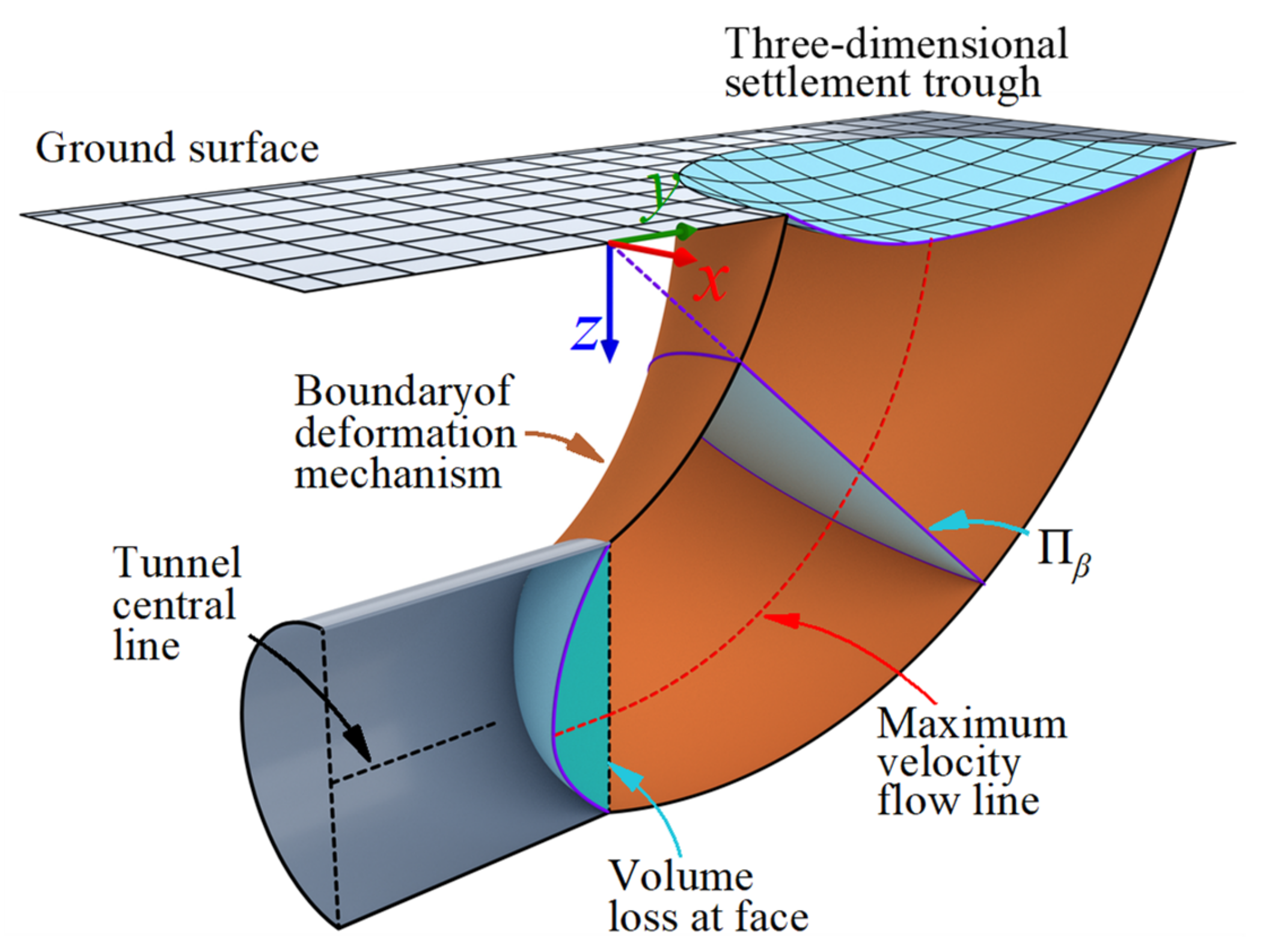
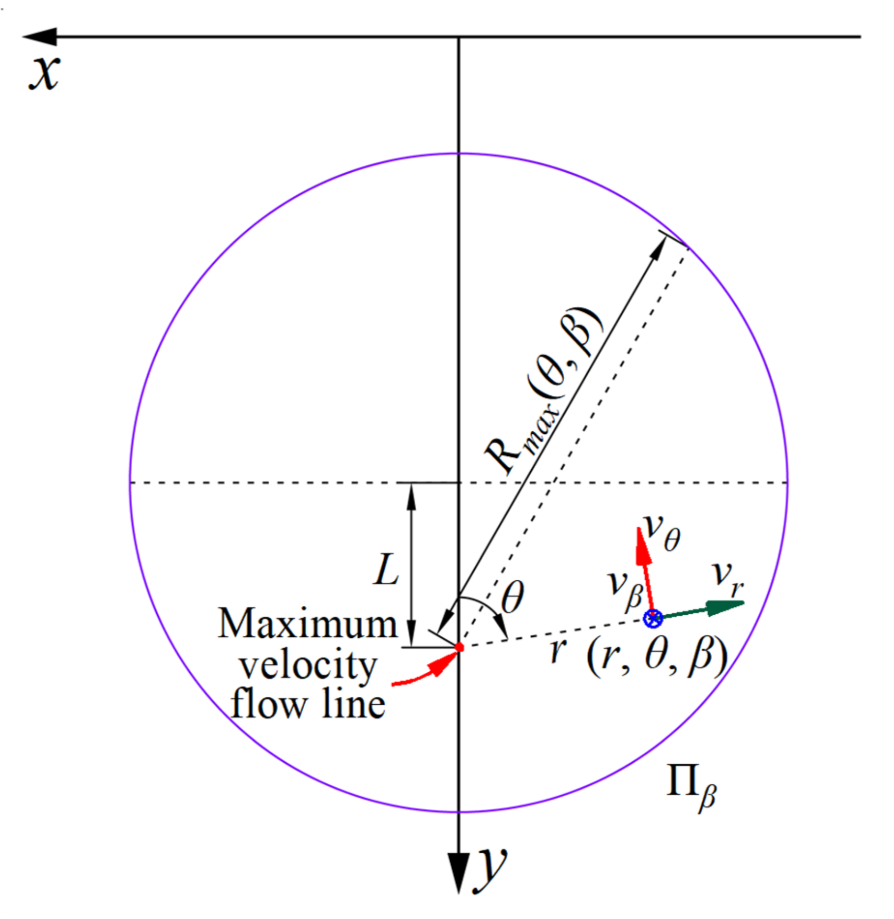
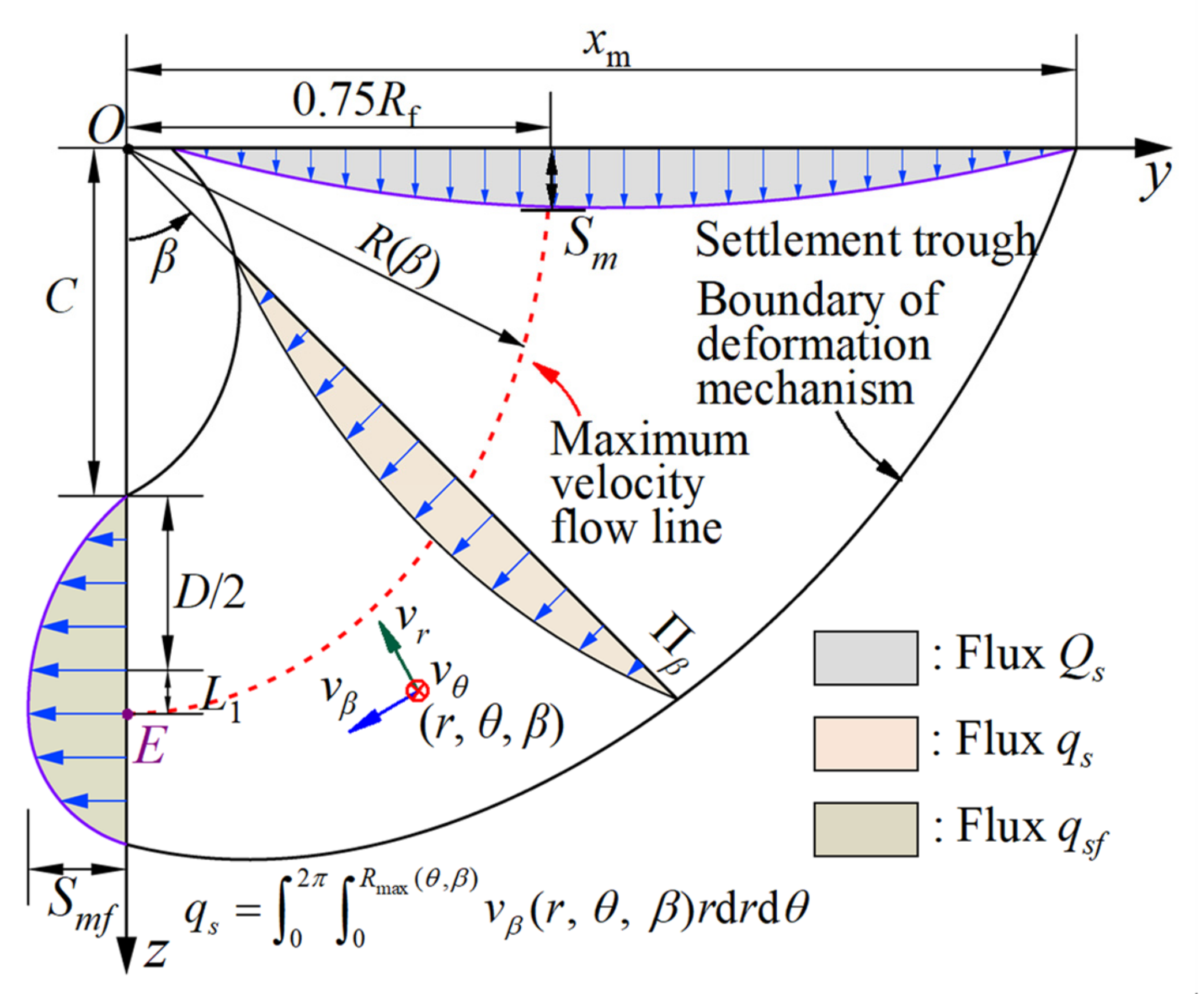
4. Deformation Mechanism

4.1. Deformaiton Mechanism

Two different continuous velocity fields for the collapse of a pressurized tunnel face were constructed [29]. The first velocity field, M1, assumed that the point with maximum velocity was located at the center of the tunnel face. The second velocity field was more suitable for engineer projects, because it assumed that the point with maximum velocity was located below the center of the tunnel face. However, the M2 velocity field was designed for collapse, and ignored the volume change of soil. A new deformation mechanism (Figure 3) was designed based on the modification of the M2 velocity field. The new deformation mechanism contains several parameters which decide the geometry of the new deformation mechanism. The parameters depend on the mechanical properties of the soil.

As shown in Figure 4, the maximum displacement on the tunnel face is S_mf and is located at point E. The maximum velocity flow line is a quarter of an ellipse, with respect to the origin O. The semi-major axis of the ellipse is R_f = C + D/2 + L₁. L₁ is the distance between the center of the face and point E. The semi-minor axis of the ellipse is 0.75 R_f. For a better description of the deformation mechanism, the curvilinear coordinate system (r, θ, β) is adopted.

The new deformation mechanism assumes that the soil within the boundary flows towards the face in a toric manner, and the soil outside the boundary is rigid. The boundary is constructed by the periphery of the different circular cross-section, Π_β, as shown in Figure 5

R_max is the radius of the circular cross-section, and it can be given by Equation (6):

$$R_{\max }(\theta , \beta )=\frac{D·{\mathsf{\Omega }}_1{\mathsf{\Omega }}_2}{2{\mathsf{\Omega }}_3}$$

(6)

$${\mathsf{\Omega }}_1(\beta )=(1+2{\overline{L}}_1)(\pi -2\beta )+3\beta {\overline{R}}_f$$

(7)

$${\mathsf{\Omega }}_2(\theta ,\beta )=2\overline{L}\cos \theta +\sqrt{1-2{\overline{L}}^2+2{\overline{L}}^2\cos 2\theta }$$

(8)

$${\mathsf{\Omega }}_3=(1+2{\overline{L}}_1)\pi$$

(9)

$$\overline{L}={\overline{L}}_1-l\beta$$

(10)

where $\overline{[·]}$ means normalized with respect to tunnel diameter (such as $\overline{C}=C/D$). L indicates the distance between the point with maximum displacement and the center of the circular cross-section.

On the Π_β plane, the orthoradial displacement component (v_r) is assumed to be zero. The axial displacement component (v_β) is assumed to decrease in a parabolic way to vanish at the boundary, as shown in Figure 4. Equation (11) gives the orthoradial displacement of points (r, θ, β) on the plane Π_β:

$$v_{\beta }(r, \theta , \beta )=v_m(\beta )⟮1-\frac{r^2}{R_{\max }^2(\theta , \beta )}⟯$$

(11)

where v_m(β) is the orthoradial displacement on the maximum velocity flow line. On the face, the displacement can be expressed as follow:

$$v_{\beta }(r, \theta , 0)=S_{mf}⟮1-\frac{r^2}{R_{\max }^2(\theta , 0)}⟯$$

(12)

where S_mf is the maximum displacement on the face. Furthermore, the flux across the tunnel face (q_sf) can be acquired by integral Equation (13) over the tunnel face.

$$q_{sf}=S_{mf}·\frac{\pi D^2}{8}$$

(13)

In previous deformation mechanism [29], the assumption of zero volume change was made and the flux through any Π_β plane was the same. However, as drainage or volume loss always happens in the sand, we assume that the flux across plane Π_β linearly increases (or decreases) with β:

$$q_s=q_{sf}(k\beta +1)=S_{mf}·\frac{\pi D^2}{8}(k\beta +1)$$

(14)

where k is used to describe the extent of the volume change of the soil, and q_s denotes the flux through plane Π_β. At the tunnel face, q_s is equal to q_sf. q_s equal to Q_s at the ground surface.

$$\begin{array}{ll}{q}_s& ={\displaystyle {\int }_0^{2\pi }{\displaystyle {\int }_0^{R_{\max }(\theta ,\beta )}{v}_{\beta }(r, \theta , \beta )}r\mathrm{d}r\mathrm{d}\theta }\\ & ={\displaystyle {\int }_0^{2\pi }{\displaystyle {\int }_0^{R_{\max }(\theta ,\beta )}{v}_m(\beta )⟮1-\frac{r^2}{R_{\max }^2(\theta , \beta )}⟯r\mathrm{d}r\mathrm{d}\theta }}\\ & =v_m(\beta ){\displaystyle {\int }_0^{2\pi }{\displaystyle {\int }_0^{R_{\max }(\theta ,\beta )}⟮1-\frac{r^2}{R_{\max }^2(\theta , \beta )}⟯r\mathrm{d}r\mathrm{d}\theta }}\\ & =v_m(\beta )\frac{\pi D^2{\mathsf{\Omega }}_1^2}{8{\mathsf{\Omega }}_3^2}\end{array}$$

(15)

So, combining Equations (14) and (15), the maximum orthoradial displacement on any plane can be given by Equation (16).

$$v_m(\beta )=\frac{S_{\mathrm{mf}}(k\beta +1){\mathsf{\Omega }}_3^2}{{\mathsf{\Omega }}_1^2}$$

(16)

So, v_β can be derived as follows.

$$v_{\beta }(r, \theta , \beta )=\frac{S_{\mathrm{mf}}(k\beta +1){\mathsf{\Omega }}_3^2}{{\mathsf{\Omega }}_1^2}⟮1-\frac{r^2}{R_{\max }^2(\theta , \beta )}⟯$$

(17)

In solid mechanics, there are two expressions for the volumetric strain (Θ): the ratio of the volume change (∆V) to the original volume (V), and the summation of the normal strains in three mutually perpendicular directions, as shown in Equation (18).

$$\mathsf{\Theta }=\frac{\Delta V}{V}={\epsilon }_r+{\epsilon }_{\theta }+{\epsilon }_{\beta }$$

(18)

Moreover, the volume change (∆V) of the Π_β plane with dβ can be calculated by taking the derivative of q_s as shown in Equation (19).

$$\Delta V=\frac{\partial q_s}{\partial \beta }·\mathrm{d}\beta =q_{sf}k·\mathrm{d}\beta$$

(19)

The original volume of the Π_β plane with dβ can be given as follows:

$$V=\mathrm{d}\beta ·R_f·D_s{(\beta )}^2\pi /4$$

(20)

where D_S(β) is the diameter of the Π_β plane, and can be expressed as follows.

$$D_s(\beta )=R_{\max }(\theta =0, \beta )+R_{\max }(\theta =\frac{\pi }{2}, \beta )=\frac{{\mathsf{\Omega }}_{1}D}{{\mathsf{\Omega }}_3}$$

(21)

So, we have:

$$\mathsf{\Theta }=\frac{S_{\mathrm{mf}}·k{\mathsf{\Omega }}_3^2}{2R_{\mathrm{f}}{\mathsf{\Omega }}_1^2}$$

(22)

The second expression of the volumetric volume shown in Equation (18) can be calculated by the strain introduced in Section 4.2. The volumetric volume can be also given as follows.

$$\frac{\partial v_r}{\partial r}+\frac{1}{r}{v}_r+\frac{1}{R_{\beta }-r\cos \theta }(-{\upsilon }_r\cos \theta +\frac{\partial {\upsilon }_{\beta }}{\partial \beta })=\mathsf{\Theta }$$

(23)

After simplification of Equation (23), we have:

$$\frac{\partial v_r}{\partial \overline{r}}+\frac{({\overline{R}}_{\beta }-2\overline{r}\cos \theta )}{\overline{r}({\overline{R}}_{\beta }-\overline{r}\cos \theta )}{v}_r=-\frac{1}{({\overline{R}}_{\beta }-\overline{r}\cos \theta )}\frac{\partial v_{\beta }}{\partial \beta }+\frac{S_{\mathrm{mf}}·k{\mathsf{\Omega }}_3^2}{2{\overline{R}}_{\beta }{\mathsf{\Omega }}_1^2}$$

(24)

The derivative of orthoradial displacement v_β with respect to β can be given as follows:

$$\begin{array}{ll}\frac{\partial v_{\beta }}{\partial \beta }& =S_{\mathrm{mf}}\frac{{\mathsf{\Omega }}_3^2}{{\mathsf{\Omega }}_1^2}\left[k⟮1-\frac{4{\mathsf{\Omega }}_3^2{\overline{r}}^2}{{\mathsf{\Omega }}_1^4{\mathsf{\Omega }}_2^2}⟯+(k\beta +1)⟮-2{\mathsf{\Omega }}_4-\frac{4{\mathsf{\Omega }}_3^2{\mathsf{\Omega }}_5{\overline{r}}^2}{{\mathsf{\Omega }}_1^5{\mathsf{\Omega }}_2^3}⟯\right]\\ & =S_{\mathrm{mf}}\frac{{\mathsf{\Omega }}_3^2}{{\mathsf{\Omega }}_1^2}\left[-4\frac{{\mathsf{\Omega }}_3^2}{{\mathsf{\Omega }}_1^4{\mathsf{\Omega }}_2^2}\left(k+\frac{(k\beta +1){\mathsf{\Omega }}_5}{{\mathsf{\Omega }}_1{\mathsf{\Omega }}_2}\right){\overline{r}}^2+k-2(k\beta +1){\mathsf{\Omega }}_4\right]\end{array}$$

(25)

$${\mathsf{\Omega }}_5(\theta ,\beta )=-4{\mathsf{\Omega }}_2{\mathsf{\Omega }}_4+3{\mathsf{\Omega }}_1⟮\cos \theta +\frac{2\overline{L}{\sin }^2\theta }{\sqrt{1-2{\overline{L}}^2+2{\overline{L}}^2\cos 2\theta }}⟯$$

(26)

Equation (24) is an ordinary first-order linear differential equation. In order to simplify the calculation, Equation (24) can be expressed as follows:

$$\frac{\partial v_r}{\partial \overline{r}}+\frac{({\overline{R}}_{\beta }-2\overline{r}\cos \theta )}{\overline{r}({\overline{R}}_{\beta }-\overline{r}\cos \theta )}{v}_r=-\frac{1}{({\overline{R}}_{\beta }-\overline{r}\cos \theta )}\left(A{\overline{r}}^2+B\right)+\mathsf{\Theta }$$

(27)

where A and B can be given as follows:

$$\left\{\begin{array}{l}A=-4S_{\mathrm{mf}}\frac{{\mathsf{\Omega }}_3^4}{{\mathsf{\Omega }}_1^6{\mathsf{\Omega }}_2^2}⟮k+\frac{(k\beta +1){\mathsf{\Omega }}_5}{{\mathsf{\Omega }}_1{\mathsf{\Omega }}_2}⟯\\ B=S_{\mathrm{mf}}\frac{{\mathsf{\Omega }}_3^2}{{\mathsf{\Omega }}_1^2}\left(k-2(k\beta +1){\mathsf{\Omega }}_4\right)\end{array}\right.$$

(28)

Solving it with boundary condition v_r(R_max(θ, β), θ, β) = 0, we have:

$$v_r(r,\theta ,\beta )=\frac{6(B-\mathsf{\Theta }{\overline{R}}_{\beta }){(\overline{r}-R_{\max })}^2+4\cos \theta ·{(\overline{r}-R_{\max })}^3+3A{(\overline{r}-R_{\max })}^4}{12({\overline{R}}_{\beta }-\overline{r}\cos \theta )}$$

(29)

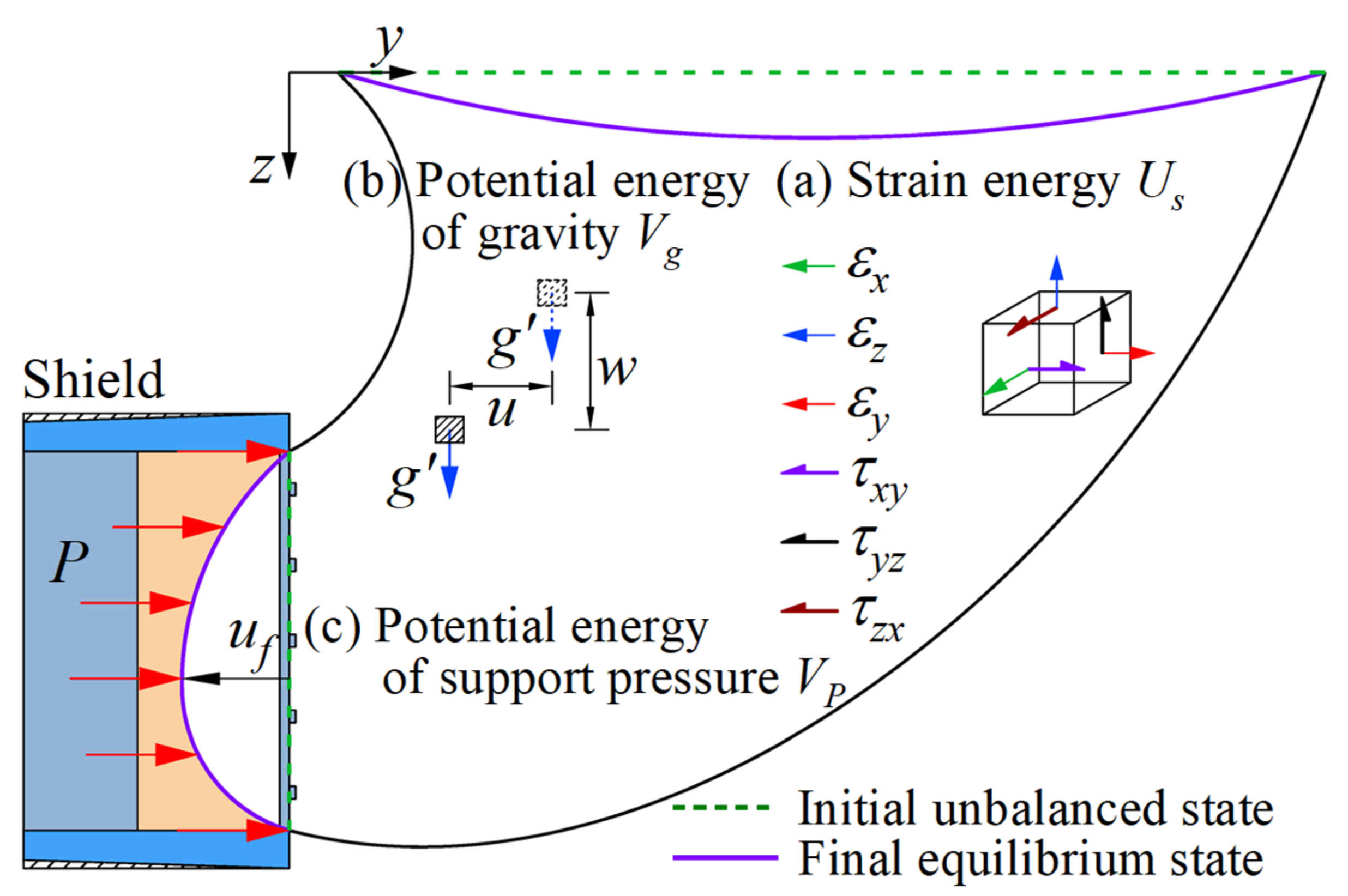
4.2. Calculation of Potential Energy

(a)

Strain energy

Because the strain of the soil is derived from the deformation mechanism, and the deformation mechanism in this paper is expressed in a curvilinear coordinate system, we have to convert the strain in the curvilinear coordinate system to the strain in the Cartesian coordinate system. Equation (30) gives the relationship between the curvilinear coordinate system and the Cartesian coordinate system.

$$\left\{\begin{array}{l}x=-r\sin \theta \\ y=(R_{\beta }-r\cos \theta )\cos \beta \\ z=(R_{\beta }-r\cos \theta )\sin \beta \end{array}\right.$$

(30)

$$R_{\beta }={\left({\cos }^2\beta /R_f^2+{\cos }^2\beta /{(0.75R_f)}^2\right)}^{-0.5}$$

(31)

The conversion can be easily given by tensor calculation, as shown in Equations (32) and (33).

$$\left[\begin{array}{ccc}{\epsilon }_x& {\epsilon }_{xy}& {\epsilon }_{xz}\\ {\epsilon }_{yx}& {\epsilon }_y& {\epsilon }_{yz}\\ {\epsilon }_{zx}& {\epsilon }_{zy}& {\epsilon }_z\end{array}\right]=P\left[\begin{array}{ccc}{\epsilon }_r& {\epsilon }_{ry}& {\epsilon }_{rz}\\ {\epsilon }_{\theta r}& {\epsilon }_{\theta }& {\epsilon }_{\theta \beta }\\ {\epsilon }_{\beta r}& {\epsilon }_{\beta \theta }& {\epsilon }_{\beta }\end{array}\right]P^T$$

(32)

$$P=\left[\begin{array}{ccc}-\sin \theta & \cos \beta \cos \theta & \cos \theta \sin \beta \\ \cos \theta & \cos \beta \sin \theta & -\sin \beta \sin \theta \\ 0& \sin \beta & \cos \beta \end{array}\right]$$

(33)

Klar and Klein [28] derived the geometrical equations in the curvilinear coordinate system. Based on the work performed by Klar and Klein [28], we give the geometrical equations modified for the coordinate in our method as follows.

$$\left\{\begin{array}{l}{\epsilon }_{rr}=\frac{\partial {\upsilon }_r}{\partial r}\\ {\epsilon }_{rr}=\frac{1}{2r}⟮\frac{\partial {\upsilon }_r}{\partial \theta }+r\frac{\partial {\upsilon }_{\theta }}{\partial r}-{\upsilon }_{\theta }⟯\\ {\epsilon }_{r\beta }=\frac{1}{2(R_{\beta }-r\cos \theta )}\left[{\upsilon }_{\beta }\cos \theta +\frac{\partial {\upsilon }_r}{\partial \beta }+(R_{\beta }-r\cos \theta )\frac{\partial {\upsilon }_{\beta }}{\partial r}\right]\\ {\epsilon }_{\theta \theta }=\frac{1}{r}⟮{\upsilon }_r+\frac{\partial {\upsilon }_{\theta }}{\partial \theta }⟯\\ {\epsilon }_{\theta \beta }=\frac{1}{2r(R_{\beta }-r\cos \theta )}\left[r\frac{\partial {\upsilon }_{\theta }}{\partial \beta }-{\upsilon }_{\beta }r\sin \theta +\frac{\partial {\upsilon }_r}{\partial \beta }+(R_{\beta }-r\cos \theta )\frac{\partial {\upsilon }_{\beta }}{\partial \theta }\right]\\ {\epsilon }_{\beta \beta }=\frac{1}{R_{\beta }-r\cos \theta }⟮{\upsilon }_{\theta }\sin \theta -{\upsilon }_r\cos \theta +\frac{\partial {\upsilon }_{\beta }}{\partial \beta }⟯\end{array}\right.$$

(34)

Equation (34) gives the train energy of the soil. Equation (4), the strain energy of the soil, can be calculated by combining Equation (4) with Equation (34).

(b)

Potential energy of external force

According to the deformation mechanism, the vertical displacement can be given as follows:

$$w=-{\upsilon }_r\cos \theta \cos \beta +{\upsilon }_{\theta }\cos \beta \sin \theta -{\upsilon }_{\beta }\sin \beta$$

(35)

Substituting Equation (35) into Equation (6), the potential energy of gravity can be calculated.

When β = 0, the orthoradial displacement v_β(r, θ, β) is equal to the horizontal displacement on the tunnel face u_f. Equation (36) gives the horizontal displacement on the tunnel face.

$$u_f={\upsilon }_{\beta }(r, \theta , 0)$$

(36)

Combining Equation (36) with Equation (5), the potential energy of support pressure can be calculated.

4.3. Volume Loss Calculation

V_lf is the volume loss at the tunnel face and equals the ratio of the flux on the tunnel face (q_sf) to the area of the tunnel cross-section.

$$V_L=q_{sf}/\frac{\pi D^2}{4}=\frac{1}{2}{S}_{mf}$$

(37)

V_L is the volume loss at ground surface and equals the ratio of the flux on the ground surface (Q_s) to the area of the tunnel cross-section, as defined in Klar and Klein [28]. Q_s equals q_s (π/2). So, the volume loss can be given as follows:

$$V_L=q_{sf}(\frac{\pi }{2}k+1)/\frac{\pi D^2}{4}=\frac{1}{2}{S}_{mf}(\frac{\pi }{2}k+1)$$

(38)

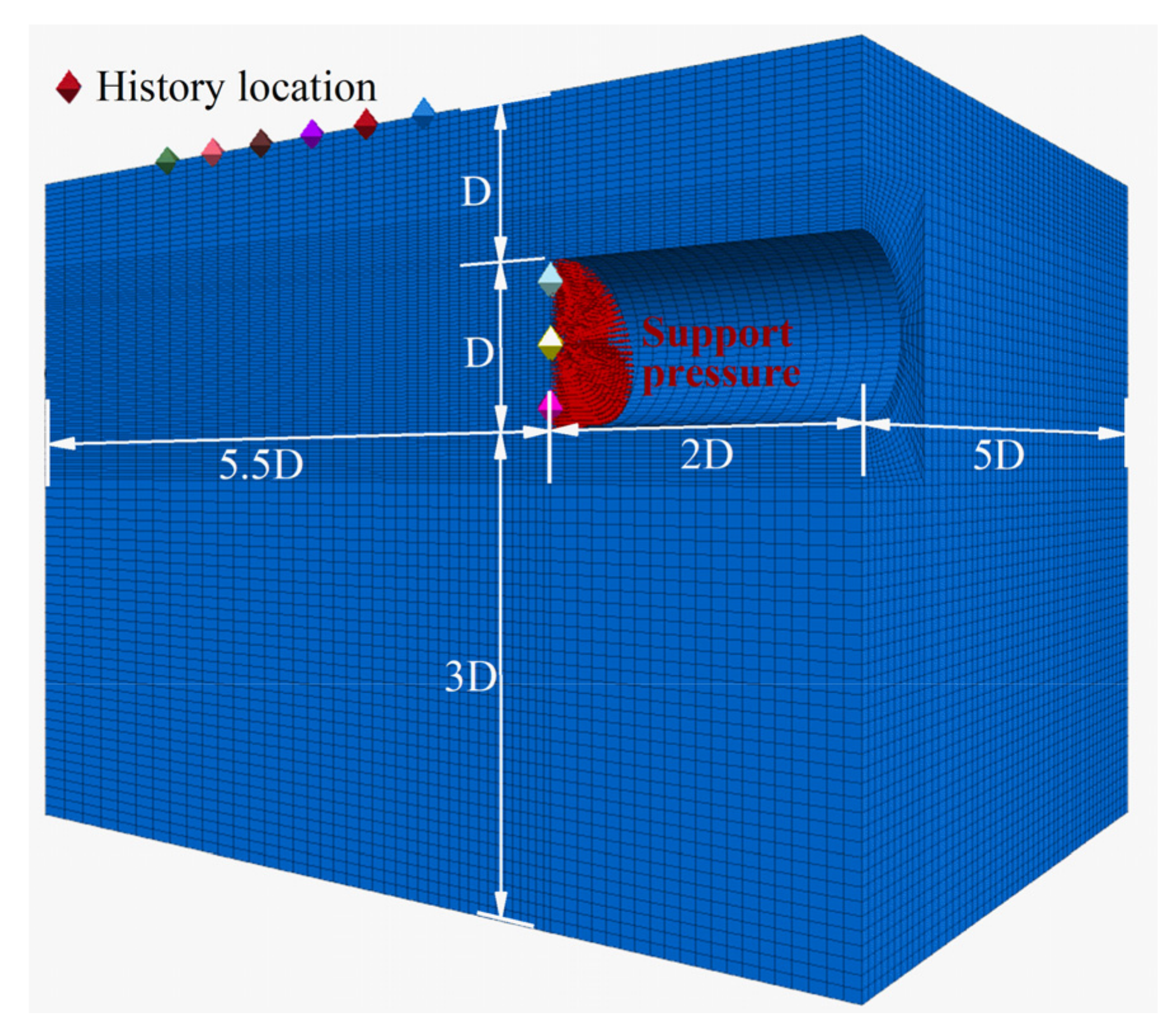
5. Verification with Numerical Simulation

In this section, we perform numerical simulations by a finite difference computer program FLAC3D to validate the accuracy of the proposed method.

As shown in Figure 6, only a half model is built due to the symmetry along the tunnel central line. The tunnel diameter and cover depth are 12 m. To guarantee the accuracy of the numerical model, the dimension size should be large enough to wake the influence of the boundary, and the specific dimension is shown in Figure 6. The mechanical parameters of the soil and support pressure are shown in

Table 1. Mechanical parameters of soil and support pressure.

Parameters	Value
Buoyant unit weight of soil (kN/m3)	18
Unit weight of water (kN/m3)	10
Elastic modulus (MPa)	1
Poisson’s ratio	0.3
Support pressure ratio	0.85, 0.9, 0.95, 1.00
Slurry weight (kN/m3)	12, 13, 14

.

In this numerical model, the top surface of the model was free, normal velocity on the four vertical surfaces was restricted, and the boundary surface was fixed. Because we focused on the displacement of soil before the tunnel face, a simplified one-step excavation was applied after reaching initial equilibrium, due to gravity. Based on the assumption that the V_Ls and V_Lt were zero, the normal displacement of points on the opening was fixed after excavation. Immediately, the gradient support pressure was applied on the face. We monitored the displacement of the points on the face and surface. The calculation was stopped when the displacements of several points were stable.

We extracted the maximum displacement on the tunnel face and ground surface in the numerical simulations, and calculated the volume loss at the tunnel face and the ground surface. The comparison is shown in Figure 7.

The comparison shows that the proposed method has a good agreement with the numerical simulation.

6. Parameter Analysis

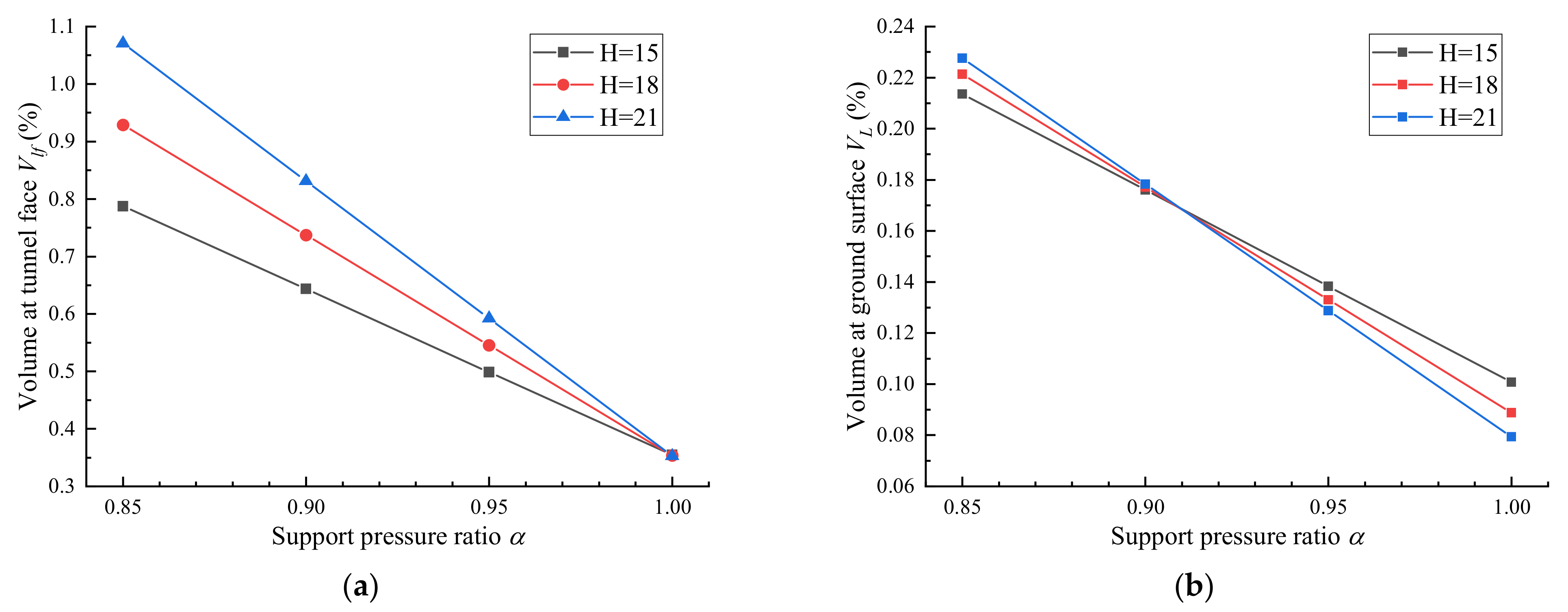
6.1. Influence of Support Pressure Ratio

The influence of the support pressure ratio α on the volume loss with the tunnel diameter ranging from 10 m to 14 m is shown in Figure 8. The tunnel depth was 15 m and the slurry weight was 12 kN/m³. The volume loss decreased linearly with the increase in the support pressure ratio, which implied that the increase in the support pressure ratio was favorable to the control of volume loss, including the volume loss at the tunnel face and the volume loss at ground surface. Moreover, the deeper the tunnel, the bigger the volume loss. The volume loss at the tunnel face is generally bigger than the volume loss at ground surface, due to the soil compression during ground movement. The influence of the tunnel diameter on the volume loss at the ground surface is much smaller than that at the tunnel face.

The influence of the support pressure ratio α on the volume loss with the tunnel depth ranging from 15 m to 21 m is shown in Figure 9. The tunnel diameter was 12 m, and the slurry weight was 12 kN/m³. With the increase in support pressure ratio, volume loss decreased linearly. Moreover, the deeper the tunnel, the faster the volume loss decreased. When α = 1, the tunnel depth did not influence the volume loss at the tunnel face. However, the tunnel depth will influence the soil compression, and the volume loss at the ground surface will be affected by the tunnel depth.

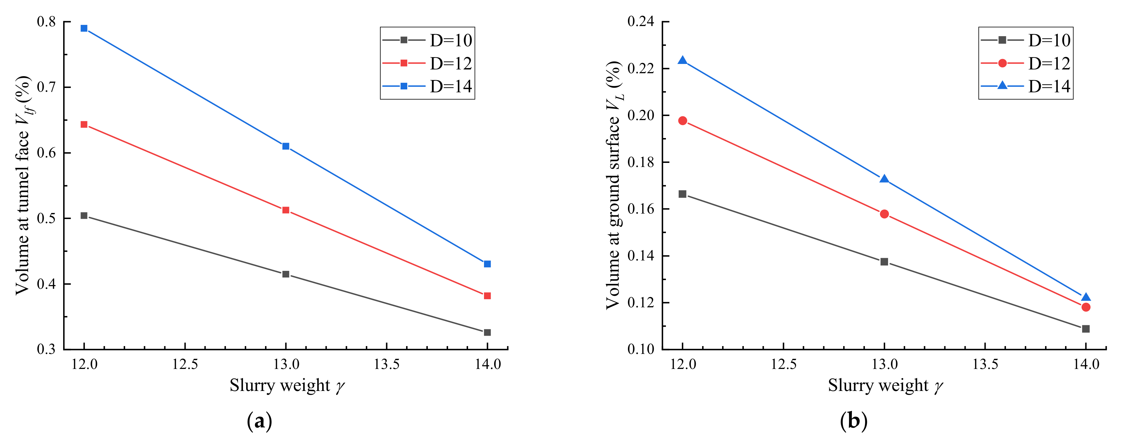
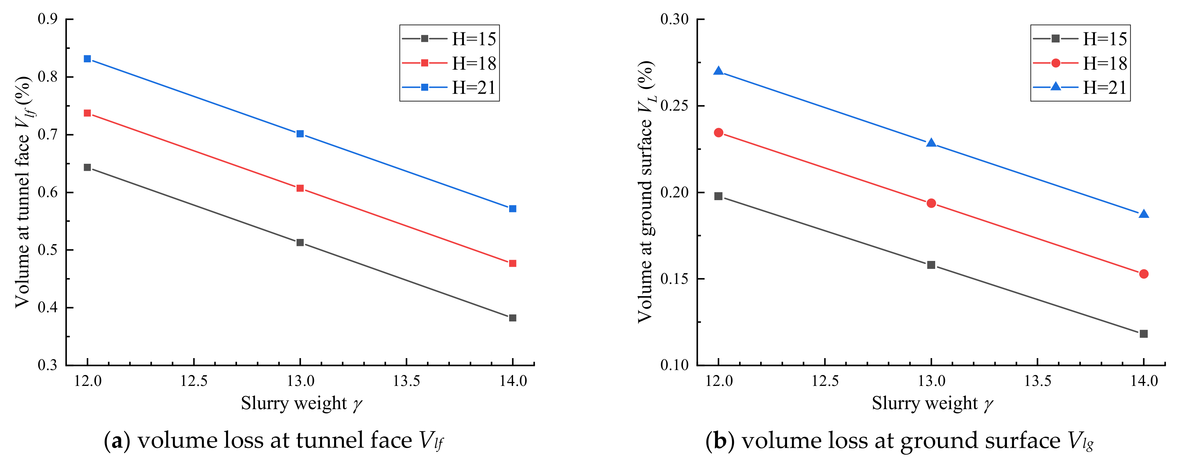
6.2. Influence of Slurry Weight

The influence of the slurry weight γ on the volume loss with the tunnel diameter ranging from 10 m to 14 m and tunnel depth ranging from 15 m to 21 m are shown in Figure 10 and Figure 11, respectively. The support pressure ratio was 0.9. The tunnel depth was 15 m in Figure 10, and tunnel diameter was 12 m in Figure 11. The volume loss decreased linearly with the increase in slurry weight, which implies that the increase in the slurry weight was favorable to the control of volume loss, including the volume loss at the tunnel face and the volume loss at the ground surface. The bigger the tunnel diameter, the quicker the volume loss decreased. However, the tunnel diameter did not influence the decrease rapidly. Moreover, the volume loss increased with the increase in the tunnel diameter and tunnel depth.

7. Conclusions

In this paper, a semi-analytical method based on the principle of minimum total potential energy was proposed to solve the volume loss at the tunnel face and the ground face for shield-driven tunnels. Moreover, a new deformation mechanism considering the soil volume change was designed to describe the ground movement before the tunnel face. Based on the proposed method, the influence of different factors on the volume loss was investigated. The main conclusions are given as follow:

The volume loss decreases with the increase in the support pressure ratio and the slurry weight. The increase in the slurry weight is favorable to the control of volume loss during tunnelling

The volume loss at ground surface is smaller than that at the tunnel face due to the soil compression during ground movement.

The bigger the tunnel diameter, the bigger the volume loss. However, the volume loss at ground surface may not increase with the increase in the tunnel depth because of the soil arching effect.

The deeper the tunnel, the quicker the volume loss decreases with the increase in the support pressure ratio. The bigger the tunnel diameter, the quicker the volume loss decreases with the increase in the slurry weight.

The proposed method provides a more direct way for estimating volume loss at the tunnel face from an energy point of view. Most current researchers have assumed zero volume behind the tunnel face (V_Lt and V_Ls), and the considered volume loss is limited to the tunnel face (‘tunnel heading’). A more effective way for estimating all volume loss along the shield advancement may be developed by designing multiple deformation mechanisms according to the field data and numerical simulations.

References

1. Sagaseta, C. Analysis of undrained soil deformation due to ground loss. Geotechnique 1988, 38, 647–649. [Google Scholar] [CrossRef]
2. Verruijt, A. A Complex Variable Solution for a Deforming Circular Tunnel in an Elastic Half-Plane. Int. J. Numer. Anal. Methods Geomech. 1997, 21, 77–89. [Google Scholar] [CrossRef]
3. Loganathan, N.; Poulos, H.G. Analytical prediction for tunneling-induced ground movements in clays. J. Geotech. Geoenviron. Eng. 1998, 124, 846–856. [Google Scholar] [CrossRef]
4. Bobet, A. Analytical Solutions for Shallow Tunnels in Saturated Ground. J. Eng. Mech. 2001, 127, 1258–1266. [Google Scholar] [CrossRef]
5. Park, K.H. Analytical solution for tunnelling-induced ground movement in clays. Tunn. Undergr. Space Technol. 2005, 20, 249–261. [Google Scholar] [CrossRef]
6. Li, S.; Li, P.; Zhang, M. Analysis of additional stress for a curved shield tunnel. Tunn. Undergr. Space Technol. 2021, 107, 103675. [Google Scholar] [CrossRef]
7. Fang, Q.; Wang, G.; Yu, F.C.; Du, J.M. Analytical algorithm for longitudinal deformation profile of a deep tunnel. J. Rock Mech. Geotech. Eng. 2021, 13, 845–854. [Google Scholar] [CrossRef]
8. Li, P.F.; Wei, Y.J.; Zhang, M.J.; Huang, Q.F.; Wang, F. Influence of non-associated flow rule on passive face instability for shallow shield tunnels. Tunn. Undergr. Space Technol. 2022, 119, 104202. [Google Scholar] [CrossRef]
9. Fang, Q.; Zhang, D.; Wong, L.N.Y. Shallow tunnelling method (STM) for subway station construction in soft ground. Tunn. Undergr. Space Technol. 2012, 29, 10–30. [Google Scholar] [CrossRef]
10. Vu, M.N.; Broere, W.; Bosch, J. Volume loss in shallow tunnelling. Tunn. Undergr. Space Technol. 2016, 59, 77–90. [Google Scholar] [CrossRef] [Green Version]
11. Fang, Q.; Du, J.M.; Li, J.Y.; Zhang, D.L.; Cao, L.Q. Settlement characteristics of large-diameter shield excavation below existing subway in close vicinity. J. Cent. South Univ. 2021, 28, 882–897. [Google Scholar] [CrossRef]
12. Gui, M.W.; Chen, S.L. Estimation of transverse ground surface settlement induced by DOT shield tunneling. Tunn. Undergr. Space Technol. 2013, 33, 119–130. [Google Scholar] [CrossRef]
13. Shahin, H.M.; Nakai, T.; Ishii, K.; Iwata, T.; Kuroi, S. Investigation of influence of tunneling on existing building and tunnel: Model tests and numerical simulations. Acta Geotech. 2016, 11, 679–692. [Google Scholar] [CrossRef]
14. Zheng, H.; Li, P.; Ma, G. Stability analysis of the middle soil pillar for asymmetric parallel tunnels by using model testing and numerical simulations. Tunn. Undergr. Space Technol. 2020, 108, 103686. [Google Scholar] [CrossRef]
15. Bezuijen, A.; Talmon, A.M. Processes around a TBM. In Geotechnical Aspects of Underground Construction in Soft Ground—Proceedings of the 6th International Symposium, IS-SHANGHAI 2008; CRC Press: Boca Raton, FL, USA, 2009; pp. 3–13. [Google Scholar]
16. Verruijt, A.; Booker, J.R. Surface settlements due to deformation of a tunnel in an elastic half plane. Geotechnique 1996, 46, 753–756. [Google Scholar] [CrossRef]
17. González, C.; Sagaseta, C. Patterns of soil deformations around tunnels. Application to the extension of Madrid Metro. Comput. Geotech. 2001, 28, 445–468. [Google Scholar] [CrossRef]
18. Lee, K.M.; Rowe, R.K.; Lo, K.Y. Subsidence owing to tunnelling. I. Estimating the gap parameter. Can. Geotech. J. 1992, 29, 929–940. [Google Scholar] [CrossRef]
19. Rowe, R.K.; Lee, K.M. Subsidence owing to tunnelling. II. Evaluation of a prediction technique. Can. Geotech. J. 1992, 29, 941–954. [Google Scholar] [CrossRef]
20. Cao, L.; Zhang, D.; Fang, Q. Semi-analytical prediction for tunnelling-induced ground movements in multi-layered clayey soils. Tunn. Undergr. Space Technol. 2020, 102, 103446. [Google Scholar] [CrossRef]
21. Mair, R.J.; Gunn, M.J.; O’Reilly, M.P. Ground movement around shallow tunnels in soft clay. Tunn. Tunn. Int. 1982, 14, 45–48. [Google Scholar]
22. Attewell, P.B.; Yeates, J.; Selby, A.R. Soil Movements Induced by Tunnelling and their Effects on Pipelines and Structures; Methuen, Inc.: New York, NY, USA, 1986. [Google Scholar]
23. Macklin, S.R. The prediction of volume loss due to tunnelling in over consolidated clay based on heading geometry and stability number. Ground Eng. 1999, 32, 30–33. [Google Scholar]
24. Dimmock, P.S.; Mair, R.J. Estimating volume loss for open-face tunnels in London Clay. Proc. Inst. Civ. Eng. Geotech. Eng. 2007, 160, 13–22. [Google Scholar] [CrossRef]
25. Osman, A.S. Predicting 2D ground movements around tunnels in undrained clay. Geotechnique 2006, 56, 597–604. [Google Scholar] [CrossRef] [Green Version]
26. Liu, X.; Fang, Q.; Zhang, D.; Liu, Y. Energy-based prediction of volume loss ratio and plastic zone dimension of shallow tunnelling. Comput. Geotech. 2020, 118, 103343. [Google Scholar] [CrossRef]
27. Palmer, A.C.; Mair, R.J. Ground movements above tunnels: A method for calculating volume loss. Can. Geotech. J. 2011, 48, 451–457. [Google Scholar] [CrossRef]
28. Klar, A.; Klein, B. Energy-based volume loss prediction for tunnel face advancement in clays. Geotechnique 2014, 64, 776–786. [Google Scholar] [CrossRef]
29. Mollon, G.; Dias, D.; Soubra, A.-H. Continuous velocity fields for collapse and blowout of a pressurized tunnel face in purely cohesive soil. Int. J. Numer. Anal. Methods Geomech. 2012, 30, 1303–1336. [Google Scholar] [CrossRef] [Green Version]
30. Attewell, P.B.; Farmer, I.W. Ground disturbance caused by shield tunnel over consolidated clay. Eng. Geol. 1974, 8, 361–381. [Google Scholar] [CrossRef]
31. Deane, A.P.; Bassett, R.H. The Heathrow Express trial tunnel. Proc. Inst. Civ. Eng. Geotech. Eng. 1995, 113, 144–156. [Google Scholar] [CrossRef]
32. Li, P.F.; Chen, K.; Wang, F.; Li, Z. An upper-bound analytical model of blow-out for a shallow tunnel in sand considering the partial failure within the face. Tunn. Undergr. Space Technol. 2019, 91, 102989. [Google Scholar] [CrossRef]
33. Yu, L.; Zhang, D.; Fang, Q.; Cao, L.; Zhang, Y.; Xu, T. Face stability of shallow tunnelling in sandy soil considering unsupported length. Tunn. Undergr. Space Technol. 2020, 102, 103445. [Google Scholar] [CrossRef]
Figure 1. Sketch of proposed problem.
Applsci 12 01794 g001
Figure 2. Schematic diagram of the proposed model.
Applsci 12 01794 g002
Figure 3. Three-dimensional schematic diagram of modified deformation mechanism.
Applsci 12 01794 g003
Figure 4. Side view of the modified deformation mechanism.
Applsci 12 01794 g004
Figure 5. Circular cross-section Πβ.
Applsci 12 01794 g005
Figure 6. Numerical model.
Applsci 12 01794 g006
Figure 7. Comparison between numerical simulation and proposed method. (a) Volume loss at tunnel face Vlf, (b) volume loss at ground surface Vlg.
Applsci 12 01794 g007
Figure 8. Volume loss versus support pressure ratio α with different tunnel diameter D. (a) volume loss at tunnel face Vlf, (b) volume loss at ground surface Vlg.
Applsci 12 01794 g008
Figure 9. Volume loss versus support pressure ratio α with different tunnel depth H. (a) Volume loss at tunnel face Vlf, (b) volume loss at ground surface Vlg.
Applsci 12 01794 g009
Figure 10. Volume loss versus slurry weight γ with different tunnel diameter D. (a) Volume loss at tunnel face Vlf, (b) volume loss at ground surface Vlg.
Applsci 12 01794 g010
Figure 11. Volume loss versus slurry weight γ with different tunnel depth H. (a) Volume loss at tunnel face Vlf, (b) volume loss at ground surface Vlg.
Applsci 12 01794 g011