Abstract
Hyperspectral imaging (HSI), measuring the reflectance over visible (VIS), near-infrared (NIR), and shortwave infrared wavelengths (SWIR), has empowered the task of classification and can be useful in a variety of application areas like agriculture, even at a minor level. Band selection (BS) refers to the process of selecting the most relevant bands from a hyperspectral image, which is a necessary and important step for classification in HSI. Though numerous successful methods are available for selecting informative bands, reflectance properties are not taken into account, which is crucial for application-specific BS. The present paper aims at crop mapping for agriculture, where physical properties of light and biological conditions of plants are considered for BS. Initially, bands were partitioned according to their wavelength boundaries in visible, near-infrared, and shortwave infrared regions. Then, bands were quantized and selected via metrics like entropy, Normalized Difference Vegetation Index (NDVI), and Modified Normalized Difference Water Index (MNDWI) from each region, respectively. A Convolutional Neural Network was designed with the finer generated sub-cube to map the selective crops. Experiments were conducted on two standard HSI datasets, Indian Pines and Salinas, to classify different types of crops from Corn, Soya, Fallow, and Romaine Lettuce classes. Quantitatively, overall accuracy between 95.97% and 99.35% was achieved for Corn and Soya classes from Indian Pines; between 94.53% and 100% was achieved for Fallow and Romaine Lettuce classes from Salinas. The effectiveness of the proposed band selection with Convolutional Neural Network (CNN) can be seen from the resulted classification maps and ablation study.
1. Introduction
Due to advancements in remote sensing image acquisition mechanisms and the growing availability of rich spectral and spatial information by using a variety of sensors, hyperspectral imaging has gained importance. In particular, Hyperspectral Image (HSI) classification has become a prominent source for practical applications in fields like agriculture, environment, forestry, mineral mapping, etc. [1,2,3,4,5].
The present paper focuses on analyzing and using HSI in the agriculture field. Accurate information about growing crops with different climate conditions and agricultural resources and with different timestamps (before, during, and after cultivation) is extremely important and useful for agricultural development. Traditional methods, like field surveys and other statistical-based analyses, are very time-consuming. Advanced remote sensing technology, including HSI, provides a suitable solution and can fill the gap [6,7,8,9,10] with solutions like crop classification.
The problem of crop classification using hyperspectral images has been addressed by researchers with various methods [11,12]. A method based on regression analysis was used to classify the variety of sugarcane crops in Brazil. This HSI data was captured using the EO-1 satellite [13]. The method, proposed in [14], is a combination of Support Vector Machine (SVM) and linear spectral models and was used successfully on the data captured from the Hyperion satellite. This method was also used to classify litchi crops in Guangzhou. Crops in the Karnataka area were classified using the Spectral Angular Mapper (SAM) classifier method for the Hyperion data [15].
The HSI sensor called Airborne Visible Infra-Red Imaging Spectrometer (AVIRIS) has recently become important in the remote sensing community. AVIRIS has high spectral bands (224 bands) and spatial resolution (20 m for Indian Pines and 3.7 m for Salinas datasets) with a wavelength range of 380–2500 nm covering VIS, NIR, and SWIR regions and hence is known to be crucial for agricultural applications [16].
Some of the crop classification methods in this connection are as follows. Combined linear and nonlinear SVM algorithms were used to classify corn crops on AVIRIS data. This method obtained moderate accuracy. Soybeans and wheat crops were classified using SVM and Markov Random Field with good accuracy for the AVIRIS HSI data [17]. Unmanned Aerial Vehicle (UAV) datasets also experimented with classifying crops like cabbage, cotton, and strawberry. High accuracy was noticed using Conditional Random fields [18,19]. Further, the Salinas data set was tested to classify different crops using a support vector machine. This method achieved a moderate level of accuracy [20]. Other methods, including spatial context support vector machines, had reasonable accuracy [21].
The above methods are insufficient to extract the required information, and it is difficult to obtain commendable results [22,23,24]. Several successful band selection methods have been introduced (to perform before classification) in the literature over the last few decades, including ranking-based approaches, clustering-based approaches, searching-based approaches, relative entropy, and information entropy-based approaches [25,26,27,28]. The optimal clustering framework was introduced in [29] for band selection and successfully applied the novel objective function with several constraints. In these methods, bands are clustered initially and then ranked according to different measures to select the representative bands from the image. All these methods work well for selecting the informative bands and hence produce high classification accuracy. However, these methods may not be suitable for application-specific classification problems. For example, in the present context, we consider crop classification as our target. It is important to adopt the band section strategy in the view of agricultural phenology, where biophysical properties of plants are also taken into consideration. This is shown in Figure 1 (Source for Figure 1a: Vegetation analysis: using vegetation indices in ENVI [16]).
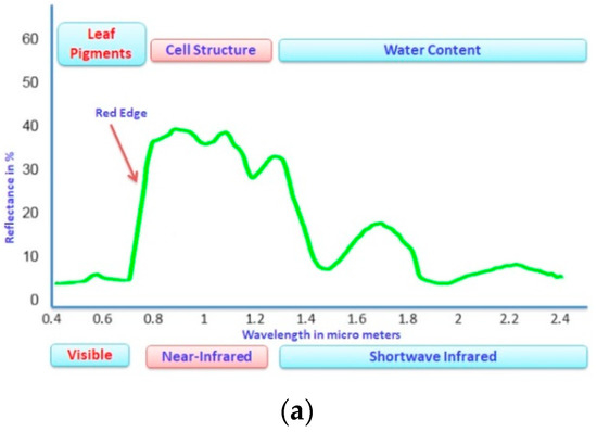
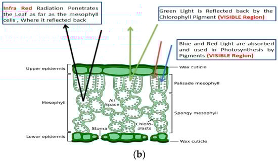
Figure 1.
(a): Spectral Reflectance Properties of Vegetation Spectrum, (b): Leaf cell structure showing the interaction of light with VIS, NIR, and SWIR regions of the electromagnetic spectrum.
The details of the measures used for the band selection, mathematical equations, range of the measures, and BS procedure are discussed in the Section 2.
The contributions of the paper are shown below:
- There are different successful methods in the literature for HSI classification. However, not all methods are suitable for all the available application areas to perform classification. In the present paper, we designed a band selection model for crop classification based on the physical and biological properties of plants.
- A new framework for informative band selection is proposed by partitioning the original hyperspectral cube based on the reflectance nature in the visible, near-infrared, and short wave infrared regions of the electromagnetic spectrum. This further uses measures such as entropy, NDVI, and NDWI, respectively, for band quantization.
- A two-dimensional convolution network for hyperspectral image classification is designed and implemented for the accurate classification of agriculture crops with the selected bands. Detailed analysis of the results in crop classification is showcased.
The following is a breakdown of the paper’s structure: materials and methods are presented in Section 2, which consists of a technical description of the proposed method. Dataset description is described in Section 3, followed by Section 4, which includes HSI classification, experimental results, and analysis. Finally, the conclusions are presented in Section 5.
2. Materials and Methods
Crop classification using HSI consists of two steps. The first is band selection, and the second is classification. Partition-based band selection is proposed in this paper. Initially, the partition is performed based on properties of the vegetation spectrum, and three partitions are created. These are termed VIS, NIR, and SWIR partitions (Figure 1). Further bands are selected from these three partitions based on three relevant metrics, entropy, NDVI, and MNDWI, respectively. In the second step to perform classification, the concatenated bands are given as input to the designed CNN model. The CNN model consists of a series of convolution and fully connected layers. Finally, crop classification can be achieved for the selected input data. The proposed architecture for the classification of crops using HSI data is shown in Figure 2.
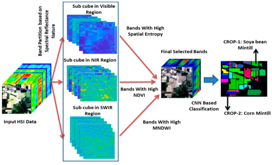
Figure 2.
Architecture of the proposed partition-based band selection and CNN-based classification for crop classification.
Let H be hyperspectral data with h rows, w columns and d represents number of spectral bands of H. Each denotes one band in the dataset. According to spectral reflectance properties in various regions of the electromagnetic spectrum, HSI data can be separated into n partitions Partition#1, Partition#2 …Partition#n with bands d1, d2,…, dn respectively. Here:
In the present context, n value is considered as 3 with Partition#1 denoting bands in the VIS region, Partition#2 denotes bands in the NIR region, and Partition#3 denotes bands in the SWIR region. Three metrics are then chosen to select bands from each partition.
Information Entropy (IE) is a criterion to measure spatial information in the HSI bands. For a particular band , Information Entropy is defined as:
where is the probability of number of grey level of the histogram of the band x in the image.
Based on IE, each band in the VIS region is quantified, and top bands are selected from Partition#1 based on the threshold limit value of δ1.
Normalized Difference Vegetation Index (NDVI) measures plant health in terms of greenness density, as shown in Equation (3). This is a widely used vegetation index in the remote sensing community. The NDVI ranges from +1 to −1. Dead plants have −1 as NDVI value, and healthy plants have values between 0.65 and 1.
Based on NDVI, each band in the NIR region is quantified, and top bands are selected from Partition#2 based on the threshold limit value of δ2.
Modified Normalized Difference Water Index (MNDWI) measures the open water enhanced identification and is computed using Equation (4). This will suppress noise generated by vegetation and soil and, at the same time, improve the open water features. MNDWI ranges from +1 to −1.
Based on MNDWI, each band in the SWIR region is quantified, and top bands are selected from Partition#3 based on the threshold limit value of δ3.
Here:
The proposed band selection algorithm is presented as Algorithm 1 below.
| Algorithm 1: Proposed Band Selection Approach for Crop Classification |
| Input: be the Hyperspectral image Data, R: Red band, G: Green band, thresholds: δ1, δ2, and δ3 |
| Output: , finer sub cube with informative and selected bands |
| Step 1: Partition the image H with d bands into three sub cubes based on light properties and biological conditions |
| Step 2: Let the number of bands in each of the sub cubes be , and bands respectively from visible, near Infrared, and shortwave infrared regions |
| Step 3: for i:1 to , Compute the entropy,, of each band using Equation (2) |
| Step 4: Generate finer sub cube with m1 bands for those bands from whose δ1 |
| Step 5: for i = 1 to , Compute the Normalized Difference Vegetation Index, using Equation (3) |
| Step 6: Generate finer sub cube with bands for those bands from whose δ2 |
| Step 7: for i = 1 to , Compute the Modified Normalized Difference Water Index, using Equation (4) |
| Step 8: Generate finer sub cube with bands for those bands from whose δ3 |
| Step 9: Combine the sub cubes , and as which satisfies Equation (5) |
There are two modules in the proposed methodology for the band selection task known as Partition and Ranking. The partition module is focused on the Biophysical properties of plants in Visible, NIR, and SWIR regions. These regions are named Partition#1, Partition#2, and Partition#3. In the ranking module, agricultural phenology metrics such as Entropy, NDVI, and MNDWI are computed using Equations (2)–(4) for the three partitions, respectively. Then, the computed values and selected representative bands are ranked using an adaptive threshold for each of the measures. The parameter tunning is shown in the experimental section.
Let denote hyperspectral data cube after the selection of m spectral bands [30,31,32]. This data can be split into two parts. One is for training and the other for testing. Let imagine χ as a training vector that will be input to the CNN model. The first layer is the convolution layer which follows according to Equation (6). Here denotes convolution operator, filter is denoted Ғ and denotes the corresponding spatial location.
Here σ (.) denotes activation function. For better convergence, the ReLU activation function is used in the present model as in Equation (7). This function gives output as same as input or zero.
After a series of convolution layers, the feature vectors are converted into a single Flatten Vector (FV), which will be given as input to Fully Connected (FC) layers. In FC layers, two operations, pre-activation and activation, will be performed at every node. All the FC layers use the ReLU activation function. However, the last layer uses the softmax activation function, as shown in Equation (8).
This function gives output probabilities of each crop, and hence classification is possible.
The proposed method performance was tested with state-of-the-art methods (a brief description of the methods is given in Section 4). The experimental works were carried out using MATLAB R 2018b and Python with Google co-laboratory. The hardware utilized for the work was a personal computer with Intel(R) Core(TM) i5-6500 CPU with 3.20 GHz and 8 GB RAM.
3. Dataset Description
In the present work, experiments were conducted using two popular AVIRIS sensor-based datasets. These datasets are freely available and can be downloaded from [33]. The first hyperspectral data used is Indian Pines. These data were captured in the agricultural area of northwestern Indiana, USA, on 12 June 1992. The number of pixels is 145*145, collected in the form of 224 bands by covering the electromagnetic spectrum in the range of 400–2500 nm. Agriculture crops like corn and soya are covered in this data as 64% area. The vegetation types of grass and pastures are covered with 25% area [34,35,36].
The second hyperspectral data used is Salinas. These data were captured in the agricultural area of the Salinas Valley region, CA, USA, on 9 October 1998. The number of pixels is 512*217, collected in the form of 224 bands by covering the electromagnetic spectrum in the range of 400–2500 nm. Agriculture crops like vineyard fields, broccoli weeds, celery, fallow, and lettuce crops are covered with 100% area [37,38,39]. The class description and pixel samples information for the two datasets is shown in Table 1 [40,41,42].

Table 1.
Number of samples per class and description of each class for two standard data sets of AVIRIS Sensor.
The major type of classes that exist in both Indian Pines and Salinas are shown in Figure 3. As per our interest for the present paper, different types of crops that exist in both Indian Pines and Salinas are also shown in Figure 4 [43,44,45,46].
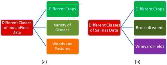
Figure 3.
Different classes of AVIRIS Sensor data (a) Indian Pines (b) Salinas.
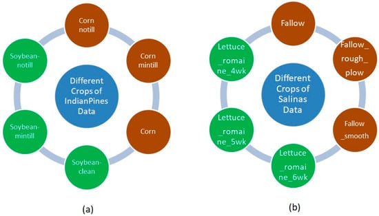
Figure 4.
Different crops of AVIRIS Sensor data (a) Indian Pines (b) Salinas.
The Indian Pines data belongs to the agricultural area of northwestern Indiana, USA. The area includes major portions of the Indian Creek and Pine Creek watersheds. Indiana is the tenth-largest farming state in the USA. More than 80% of the land in Indiana is dedicated to farms, forests, and woodland. The Salinas data belongs to one of the efficacious agricultural areas located in the central coast region of California, called the Salinas Valley, USA. This site is famous for producing most of the agricultural activities in the county due to its rich soil and plentiful underground water supplies [47].
The nomenclature for the individual classes is set according to the type of land, growing type, and spectral properties. For example, the classes “Brocoli_green_weeds_1” and “Brocoli_green_weeds_2” of Salinas’s data belong to the same type of land cover representing broccoli weeds, but they have different spectral properties due to their different conditions. The crop “Lettuce_romanine_4wk” refers to the lettuce crop that grows in the fourth week. The same terminology is used for the classes “Lettuce_romanine_5wk”, “Lettuce_romanine_6wk”, and “Lettuce_romanine_7wk”. From the Indian Pines data, “Corn-notill” represents cultivation without tillage and “Corn-mintill” represents cultivation with minimum tillage. The same terminology is used for the classes “Soybean-notill” and “Soybean-mintill”. These two classes, along with “Soybean clean”, represent different growing periods of the same soybean crop.
More information about the data and subclass regions in both datasets is presented in Figure 5.
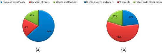
Figure 5.
Different class regions (a) Indian Pines (b) Salinas.
On the whole, it can be concluded that the selected data is more suitable for crop classification applications. Indian Pines data consists of 64% pixel regions as different types of crops, and for Salinas data, crop regions are found to be 56%.
4. Experimental Results and Analysis
This section consists of parameter tuning, complete experimental results, and analysis. Crop classification results are evaluated against standard metrics.
4.1. Subsection Parameter Tuning in Band Selection
AVIRIS Sensor data is observed to be spread over three partitions. The first partition is the visible region (VIS) in the wavelength region of 400–700 nm and is equipped with 32 bands (d1). The second partition is the near-infrared region (NIR) in the wavelength region of 700–1000 nm and is equipped with 40 bands (d2). The third partition is the short wave infrared region (SWIR) in the wavelength region of 1000–2500 nm and is equipped with 148 bands (d3).
The threshold value to select bands from the VIS region is set as 4.6 (δ1), and the number of bands selected is 15 (m1) for Indian Pines data, and for Salinas data, these values are set as 4 and 12, respectively. The threshold value to select bands from the NIR region is set as 0.2 (δ2), and the number of bands selected is 15 (m2) for Indian Pines data, and for Salinas data, these values are set as 0.11 and 16, respectively. The threshold value to select bands from the SWIR region is set as 0.62 (δ3), and the number of bands selected is 15 (m3) for Indian Pines data, and for Salinas data, these values are set as 0.99 and 15, respectively.
The red band and green band information is essential to calculate NDVI and MNDWI. These are shown in Figure 6 for both datasets [48,49].
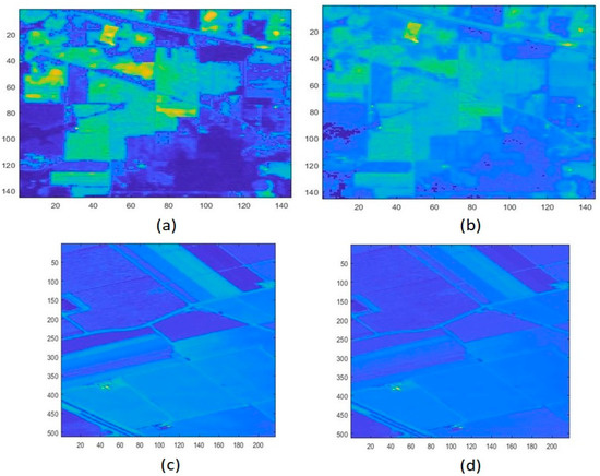
Figure 6.
Different bands of Indian Pines data. (a) Red band with band number 29, (b) Green band with band number 15. For Salinas data (c) Red band with band number 29, (d) Green band with band number 15.
The δ1, δ2, and δ3 values were set as shown in Figure 7. Using the number of available bands (224) from the AVIRIS Sensor, we considered 1/5th of the number of the bands. Accordingly, we set m1, m2, and m3 values.
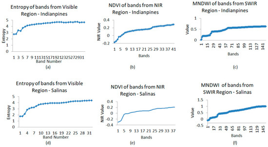
Figure 7.
Row-1: Indian Pines data (a) Entropy of visible region bands (b) NDVI of NIR region bands (c) MNDWI of SWIR region bands. Row-2: Salinas’s data (d) Entropy of visible region bands (e) NDVI of NIR region bands (f) MNDWI of SWIR region bands (Bands on x-axis for (b,c,e,f) are the chosen bands from the respective region).
From Indian Pines data, a total of 45 (m) bands were chosen with following band numbers:
18 19 20 21 22 23 24 25 26 27 28 29 30 31 32 37 38 39 41 42 43 44 45 47 48 49 50 51 52 53 151 152 153 154 155 156 157 158 159 160 161 162 163 219 220.
From Salinas data, a total of 42 (m) bands were chosen with following band numbers:
21 22 23 24 25 26 27 28 29 30 31 32 40 41 42 44 45 46 47 48 50 51 52 53 54 55 56 108 109 110 154 155 156 157 158 159 160 161 162 163 164 165.
The graphical representation, which shows the entropy of visible region bands, NDVI of NIR region bands, and MNDWI of SWIR region bands, is in Figure 7 for both datasets.
4.2. Parameter Tuning in Classification Using CNN
After the selection of representative bands, it is necessary to perform classification. The detail of the split between training and testing samples of both datasets is presented in Table 2.
Table 2.
Details of training and testing samples per band for the data sets.
Parameter tuning for common parameters of the CNN model is presented in Table 3.
Table 3.
Selected Parameters for CNN Model for two data sets.
CNN network model for Indian Pines data is presented in Table 4, and the CNN network model for Salinas data is presented in Table 5.
Table 4.
CNN Model used for Indian Pines data.
Table 5.
CNN Model used for Salinas data.
4.3. Results with Accuracy Measures
In this work, we used both quantitative and qualitative result analysis to show the performance of the proposed approach for crop classification. Three standard evaluation quantitative metrics were used [42] and are defined as:
- Overall Accuracy (OA): The percentage of correctly labeled pixels in the crop classification;
- Average Accuracy (AA): Average percentage of correctly labeled pixels for each crop;
- Class-wise Accuracies (CA): Percentage of correctly labeled pixels in each crop.
The OA, AA, and CA values of Indian Pines and Salinas, along with execution time, are shown in Table 6.
Table 6.
Details of class-wise accuracy of Indian Pines and Salinas data.
The qualitative metric used in this work is the classification map. Figure 7 shows the classification map of the Indian Pines data, and Figure 8 shows the classification map of the Salinas data [49,50,51].
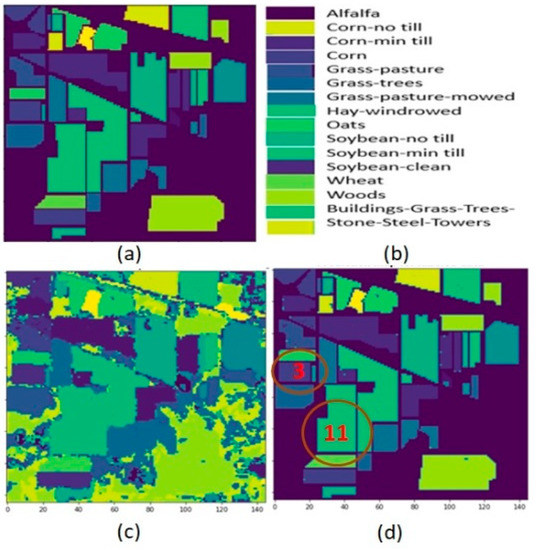
Figure 8.
Indian Pines data (a) Ground truth (b) Category label (c) Crop classification result on entire data (d) Crop classification result.
For Indian Pines data, the highest classification result was obtained for two crop classes: (Corn-mintill: class number “3”) with an accuracy of 97.12%, and (Soybean-mintill: class number “11”) with an accuracy of 99.35%. These two crop class regions are circled in Figure 8d of the classification map result.
For Salinas data, the highest classification result was obtained for two crop classes: (Fallow_rough_plow: class number “4”) with an accuracy of 100%, and (Lettuce_romaine_6wk: class number “13”) with an accuracy of 100%. These two crop class regions are pointed out in Figure 9d of the classification map result.
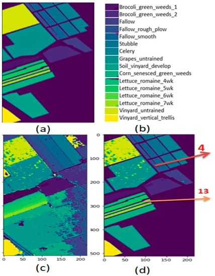
Figure 9.
Salinas data (a) Ground truth (b) Category label (c) Crop classification result on entire data (d) Crop classification result.
4.4. Discussion
This subsection discusses the classification accuracies of classes from the two datasets and also elaborates on the comparison of the proposed framework with the state-of-the-art methods.
From the Indian Pines data, it was observed that there are 6 types of crops, Corn-notill, Corn-mintill, Corn, Soybean-notill, Soybean-mintill, and Soybean-clean, with class numbers 2, 3, 4, 10, 11, and 12. The robust implementation of the classification method resulted in accuracies of 96.64%, 97.12%, 96.67%, 97.94%, 99.67%, and 95.97%, respectively. The accuracy range was found to be 95.97–99.35%.
From the Salinas data, it was observed that there are 6 types of crops, Fallow, Fallow_rough_plow, Fallow_smooth, Lettuce_romaine_4wk, Lettuce_romaine_5wk, and Lettuce_romaine_6wk, with class numbers 3, 4, 5, 11, 12, and 13. The robust implementation of the classification method resulted in accuracies of 94.53%, 100%, 99.25%, 96.52%, 97.51%, and 100%, respectively. The accuracy range was found to be 94.53–100%.
The proposed method for HSI classifications was compared with four state-of-the-art methods, including 3DGSVM [52], CNN-MFL [53], SS3FC [54], and WEDCT-MI [30], to prove the effectiveness in classifying the different crop regions.
The first method used for the comparison is the integration of 3-dimensional discrete wavelet transform and Markov random field for hyperspectral image classification called 3DGSVM [52]. In this work, more importance was given to spatial information. 3DDWT is used to extract spatial features. Probabilistic SVM coupled with MRF-based post-processing was used for HSI classification.
The second method used for the comparison is Hyperspectral Image Classification Using Convolutional Neural Networks and Multiple Feature Learning called CNN-MFL [53]. In this work, multiple features were extracted first, followed by several CNN blocks for each set of features. Here, geometric features were incorporated using attribute profiles. This is a novel technique that takes advantage of multiple feature learning and CNN to perform accurate HSI classification.
The third method used for the comparison is Spectral–Spatial Exploration for Hyperspectral Image Classification via the Fusion of Fully Convolutional Networks called SS3FC [54]. This method used spectral, spatial, and semantic information along with Fusion of Fully Convolutional Networks for HSI classification. A novel technique for the balanced splitting of the training/test dataset was introduced to solve the insufficient training samples problem.
The fourth method used for the comparison is unsupervised band selection based on weighted information entropy and 3D discrete cosine transform for hyperspectral image classification called WEDCT-MI [30]. In this work, original HSI data was first converted in discrete cosine transform-based coefficient matrices. The weighted entropy was calculated to quantify each band. Then, top-ranked bands were selected. Finally, SVM was used for classification.
Figure 10 shows the crop classification from Indian Pines and Salinas datasets. It can be seen from Figure 10 that the proposed band selection approach is effective in extracting the bands which contain much information about the crops. This is due to the inclusion of the physical properties of light in partitioning the bands and the biological properties of plants in band quantization.
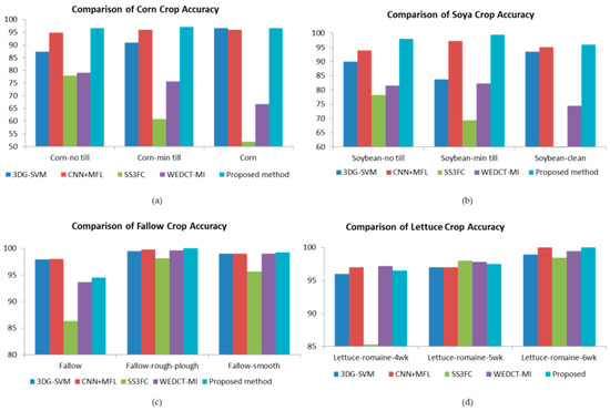
Figure 10.
Comparison of crop classification accuracy Indian Pines: (a) Corn (b) Soya Salinas (c) Fallow (d) Lettuce.
4.5. Crop-Wise Analysis
The crop-wise analysis [55] on the two datasets is shown in this subsection.
4.5.1. Corn Crops
The first crop used for the comparison is “Corn-notill,” class number 2 from the Indian Pines data. For this crop, the proposed method outperformed the state-of-the-art methods 3DGSVM, SS3FC, and WEDCT-MI with higher accuracy of 96.64%. The CNN-MFL method had 94.82% accuracy, which is on par with the proposed method. The second crop used for the comparison is “Corn-mintill”, class number 3 from the Indian Pines data. For this crop, the proposed method outperformed the state-of-the-art methods 3DGSVM, SS3FC, and WEDCT-MI with higher accuracy of 97.12%. The CNN-MFL method had 96% accuracy, which is on par with the proposed method. The third crop used for the comparison is “Corn”, class number 4 from the Indian Pines data. For this crop, the proposed method outperformed the state-of-the-art methods SS3FC and WEDCT-MI with higher accuracy of 96.67%. The methods 3DGSVM and CNN-MFL had 96.64% and 96% accuracy, respectively, which are on par with the proposed method.
4.5.2. Soya Crops
The first crop used for the comparison is “Soybean-no till”, class number 10 from the Indian Pines data. For this crop, the proposed method outperformed the state-of-the-art methods 3DGSVM, CNN-MFL, SS3FC, and WEDCT-MI with higher accuracy of 97.94%. The second crop used for the comparison is “Soybean-min till”, class number 11 from Indian Pines data. For this crop, the proposed method outperformed the state-of-the-art methods 3DGSVM, SS3FC, and WEDCT-MI with higher accuracy of 99.35%. The third crop used for the comparison is “Soybean-clean”, class number 12 from the Indian Pines data. For this crop, the proposed method outperformed the state-of-the-art methods 3DGSVM, SS3FC, and WEDCT-MI with higher accuracy of 95.97%. The method CNN-MFL had 95% accuracy, which is on par with the proposed method.
4.5.3. Fallow Crops
The first crop used for the comparison is “Fallow”, class number 3 from the Salinas data. For this crop, the proposed method outperformed the state-of-the-art methods SS3FC and WEDCT-MI with higher accuracy of 94.53%. The methods 3DGSVM and CNN-MFL were slightly more accurate than the proposed method. The second crop used for the comparison “Fallow-rough-plough”, class number 4 from the Salinas data. For this crop, the proposed method outperformed the state-of-the-art methods 3DGSVM, CNN-MFL, SS3FC, and WEDCT-MI with higher accuracy of 100%. The third crop used for the comparison was “Fallow-smooth”, class number 5 from the Salinas data. For this crop, the proposed method outperformed the state-of-the-art methods 3DGSVM, CNN-MFL, and SS3FC with higher accuracy of 99.25%. The method WEDCT-MI had 99.03% accuracy, which is on par with the proposed method.
4.5.4. Lettuce Romaine Crops
The first crop used for the comparison is “Lettuce-romaine-4wk”, class number 11 from the Salinas data. For this crop, the proposed method outperformed the state-of-the-art methods 3DGSVM and SS3FC with higher accuracy of 96.52%. Methods CNN-MFL and WEDCT-MI were slightly more accurate than the proposed method. The second crop used for the comparison is “Lettuce-romaine-5wk”, class number 12 from the Salinas data. For this crop, the proposed method outperformed the state-of-the-art methods 3DGSVM, CNN-MFL, and WEDCT-MI with higher accuracy of 97.51%. Method SS3FC was slightly more accurate than the proposed method. The third crop used for the comparison is “Lettuce-romaine-6wk”, class number 13 from the Salinas data. For this crop, the proposed method and CNN-MFL had 100% accuracy and outperformed the remaining state-of-the-art methods.
4.6. Ablation Study
We conducted an ablation study to verify the effectiveness of the proposed band selection. There are two modules in the proposed methodology known as Partition and Ranking. We conducted experiments by varying the modules (replace Proposed partition based on VIS, NIR, and SWIR regions into Coarser partition into 3 regions and replace Proposed ranking based on Entropy, NDVI, and NDWI into random selection). The ablation analysis for Indian Pines and Salinas data is shown in Table 7. The accuracy values show that the proposed band selection method has a positive impact on the hyperspectral classification.
Table 7.
Ablation experiments of proposed network.
4.7. Application of Proposed Methodology with Other Satellite Data
In order to test the adaptability and the effectiveness as in [56], we applied the proposed framework on the WHU-Hi-HongHu dataset [57,58,59]. This data consists of a complex agricultural area with a variety of crops. The data were acquired in Honghu City, China. The number of pixels is 940 × 475, with 270 bands acquired from 400 to 1000 nm wavelength. The data were acquired using an unmanned aerial vehicle (UAV)-borne hyperspectral system with high spatial resolution of 0.043 m. Out of 22 class regions, 15 classes were found with class numbers 4, 6, 7, 8, 9, 10, 11, 12, 13, 14, 16, 17, 18, 19, 20. Table 8 shows class-wise accuracies after the application of the proposed framework on the WHU-Hi-Hong Hu dataset. We used all the parameters similar to the Indian Pines and Salinas datasets. It can be concluded that the proposed framework was successful in classifying, with an average accuracy of 98.56% for 15 crop classes.
Table 8.
Ablation experiments of the proposed network.
5. Conclusions
In this paper, an approach for crop classification for HSI images is proposed. Firstly, the bands are selected based on agricultural phenology, where biophysical properties of plants are also taken into consideration. Then, a two-dimensional CNN is trained with the extracted bands. The proposed method is tested and validated on two benchmark datasets. The average accuracy of the crops corn and soya from Indian Pines is 96.81% and 97.75%. For the Salinas dataset, the average accuracy of the crops fallow and lettuce romaine is 97.93% and 98.01%, respectively. The results clearly show the effectiveness of the proposed band selection in selecting the required features necessary for crop classification. In the future, we can incorporate spatial information along with spectral information and extend it to more crops from the datasets.
Author Contributions
Conceptualization, L.A.; Data curation, L.A.; Funding acquisition, L.A. and A.F.; Methodology, V.R. and K.L.N.B.P.; Project administration, M.P.; Resources, A.F.; Software, A.F.; Supervision, M.P.; Validation, V.R. and K.L.N.B.P.; Writing—original draft, V.R. and K.L.N.B.P.; Writing—review & editing, M.P. All authors have read and agreed to the published version of the manuscript.
Funding
This research received no external funding.
Institutional Review Board Statement
Not applicable.
Informed Consent Statement
Not applicable.
Data Availability Statement
Not applicable.
Acknowledgments
The authors thank the Vellore Institute of Technology, Vellore for providing a VIT seed grant for carrying out this research work.
Conflicts of Interest
The authors declare no conflict of interest.
References
- Hoffer, R.M. Biological and physical considerations in applying computer-aided analysis techniques to remote sensor data. In Remote Sensing: The Quantitative Approach; Swain, P.H., Davis, S.M., Eds.; McGraw-Hill Book Company: New York, NY, USA, 1978; pp. 227–289. [Google Scholar]
- Karlovska, A.; Grinfelde, I.; Alsina, I.; Priedītis, G.; Roze, D. Plant Reflected Spectra Depending on Biological Characteristics and Growth Conditions. In Proceedings of the 7th International Scientific Conference Rural Development 2015, Kaunas, Lithuania, 19–20 November 2015. [Google Scholar] [CrossRef] [Green Version]
- Prabukumar, M.; Sawant, S.; Samiappan, S.; Agilandeeswari, L. Three-dimensional discrete cosine transform-based feature extraction for hyperspectral image classification. J. Appl. Remote Sens. 2018, 12, 046010. [Google Scholar] [CrossRef]
- Sawant, S.S.; Prabukumar, M. Band Fusion Based Hyper Spectral Image Classification. Int. J. Pure Appl. Math. 2017, 117, 71–76. [Google Scholar]
- Sawant, S.; Manoharan, P. A hybrid optimization approach for hyperspectral band selection based on wind driven optimization and modified cuckoo search optimization. Multimedia Tools Appl. 2020, 80, 1725–1748. [Google Scholar] [CrossRef]
- Prabukumar, M.; Shrutika, S. Band clustering using expectation–maximization algorithm and weighted average fusion-based feature extraction for hyperspectral image classification. J. Appl. Remote Sens. 2018, 12, 046015. [Google Scholar] [CrossRef]
- Sawant, S.S.; Prabukumar, M. A review on graph-based semi-supervised learning methods for hyperspectral image classification. Egypt. J. Remote Sens. Space Sci. 2020, 23, 243–248. [Google Scholar] [CrossRef]
- Sawant, S.; Manoharan, P. Hyperspectral band selection based on metaheuristic optimization approach. Infrared Phys. Technol. 2020, 107, 103295. [Google Scholar] [CrossRef]
- Sawant, S.S.; Manoharan, P. New framework for hyperspectral band selection using modified wind-driven optimization algorithm. Int. J. Remote Sens. 2019, 40, 7852–7873. [Google Scholar] [CrossRef]
- Sawant, S.S.; Manoharan, P.; Loganathan, A. Band selection strategies for hyperspectral image classification based on machine learning and artificial intelligent techniques—Survey. Arab. J. Geosci. 2021, 14, 646. [Google Scholar] [CrossRef]
- Makantasis, K.; Karantzalos, K.; Doulamis, A.; Doulamis, N. Deep supervised learning for hyperspectral data classification through convolutional neural networks. In Proceedings of the 2015 IEEE International Geoscience and Remote Sensing Symposium (IGARSS), Milan, Italy, 26–31 July 2015; pp. 4959–4962. [Google Scholar]
- He, K.; Zhang, X.; Ren, S.; Sun, J. Spatial Pyramid Pooling in Deep Convolutional Networks for Visual Recognition. IEEE Trans. Pattern Anal. Mach. Intell. 2015, 37, 1904–1916. [Google Scholar] [CrossRef] [PubMed] [Green Version]
- Galvao, L.S.; Formaggio, A.R.; Tisot, D.A. Discrimination of sugarcane varieties in Southeastern Brazil with EO-1 Hyperion data. Remote Sens. Environ. 2005, 94, 523–534. [Google Scholar] [CrossRef]
- Li, D.; Chen, S.; Chen, X. Research on method for extracting vegetation information based on hyperspectral remote sensing data. Trans. Chin. Soc. Agric. Eng. 2010, 26, 181–185. [Google Scholar]
- Bhojaraja, B.E.; Hegde, G. Mapping agewise discrimination of are canut crop water requirement using hyperspectral remotesensing. In Proceedings of the International Conference on Water Resources, Coastal and Ocean Engineering, Mangalore, India, 12–14 March 2015; pp. 1437–1444. [Google Scholar]
- Vegetation Analysis: Using Vegetation Indices in ENVI. Available online: https://www.l3harrisgeospatial.com/Learn/Whitepapers/Whitepaper-Detail/ArtMID/17811/ArticleID/16162/Vegetation-Analysis-Using-Vegetation-Indices-in-ENVI (accessed on 17 December 2021).
- Tarabalka, Y.; Fauvel, M.; Chanussot, J.; Benediktsson, J.A. SVM- and MRF-Based Method for Accurate Classification of Hyperspectral Images. IEEE Geosci. Remote Sens. Lett. 2010, 7, 736–740. [Google Scholar] [CrossRef] [Green Version]
- Wei, L.; Yu, M.; Zhong, Y.; Zhao, J.; Liang, Y.; Hu, X. Spatial–Spectral Fusion Based on Conditional Random Fields for the Fine Classification of Crops in UAV-Borne Hyperspectral Remote Sensing Imagery. Remote Sens. 2019, 11, 780. [Google Scholar] [CrossRef] [Green Version]
- Liang, L.I.U.; Xiao-Guang, J.I.A.N.G.; Xian-Bin, L.I.; Ling-Li, T.A.N.G. Study on Classification of Agricultural Crop by Hyperspectral Remote Sensing Data. J. Grad. Sch. Chin. Acad. Sci. 2006, 23, 484–488. [Google Scholar]
- Wei, L.; Yu, M.; Liang, Y.; Yuan, Z.; Huang, C.; Li, R.; Yu, Y. Precise Crop Classification Using Spectral-Spatial-Location Fusion Based on Conditional Random Fields for UAV-Borne Hyperspectral Remote Sensing Imagery. Remote Sens. 2019, 11, 2011. [Google Scholar] [CrossRef] [Green Version]
- Li, C.H.; Kuo, B.C.; Lin, C.T.; Huang, C.S. A Spatial–Contextual Support Vector Machine for Remotely Sensed Image Classification. IEEE Trans. Geosci. Remote Sens. 2012, 50, 784–799. [Google Scholar] [CrossRef]
- Zhao, C.; Luo, G.; Wang, Y.; Chen, C.; Wu, Z. UAV Recognition Based on Micro-Doppler Dynamic Attribute-Guided Augmentation Algorithm. Remote Sens. 2021, 13, 1205. [Google Scholar] [CrossRef]
- Singh, J.; Mahapatra, A.; Basu, S.; Banerjee, B. Assessment of Sentinel-1 and Sentinel-2 Satellite Imagery for Crop Classification in Indian Region During Kharif and Rabi Crop Cycles. In Proceedings of the IGARSS 2019—2019 IEEE International Geoscience and Remote Sensing Symposium, Yokohama, Japan, 28 July–2 August 2019; pp. 3720–3723. [Google Scholar]
- Wei, L.; Wang, K.; Lu, Q.; Liang, Y.; Li, H.; Wang, Z.; Wang, R.; Cao, L. Crops Fine Classification in Airborne Hyperspectral Imagery Based on Multi-Feature Fusion and Deep Learning. Remote Sens. 2021, 13, 2917. [Google Scholar] [CrossRef]
- Chang, C.-I.; Du, Q.; Sun, T.-L.; Althouse, M.L.G. A joint bandprioritization and band-decorrelation approach to band selection forhyperspectral image classification. IEEE Trans. Geosci. Remote Sens. 1999, 37, 2631–2641. [Google Scholar] [CrossRef] [Green Version]
- MartÌnez-UsÓ, A.; Pla, F.; Sotoca, J.M.; García-Sevilla, P. Clustering-based hyperspectral band selection using information measures IEEE Trans. Geosci. Remote Sens. 2007, 45, 4158–4171. [Google Scholar] [CrossRef]
- Xie, L.; Li, G.; Peng, L.; Chen, Q.; Tan, Y.; Xiao, M. Bandselection algorithm based on information entropy for hyperspectralimage classification. J. Appl. Remote Sens. 2017, 11, 026018. [Google Scholar] [CrossRef]
- Sheffield, C. Selecting band combinations from multi spectral data. Photogramm. Eng. Remote Sens. 1985, 58, 681–687. [Google Scholar]
- Wang, Q.; Zhang, F.; Li, X. Optimal Clustering Framework for Hyperspectral Band Selection. IEEE Trans. Geosci. Remote Sens. 2018, 56, 5910–5922. [Google Scholar] [CrossRef] [Green Version]
- Sawant, S.S.; Manoharan, P. Unsupervised band selection based on weighted information entropy and 3D discrete cosine transform for hyperspectral image classification. Int. J. Remote Sens. 2020, 41, 3948–3969. [Google Scholar] [CrossRef]
- Thenkabail, P.S.; Smith, R.B.; De Pauw, E. Hyperspectral Vegetation Indices and Their Relationships with Agricultural Crop Characteristics. Remote Sens. Environ. 2000, 71, 158–182. [Google Scholar] [CrossRef]
- Du, Y.; Zhang, Y.; Ling, F.; Wang, Q.; Li, W.; Li, X. Water Bodies’ Mapping from Sentinel-2 Imagery with Modified Normalized Difference Water Index at 10-m Spatial Resolution Produced by Sharpening the SWIR Band. Remote Sens. 2016, 8, 354. [Google Scholar] [CrossRef] [Green Version]
- Hyperspectral Remote Sensing Scenes. Available online: http://www.ehu.eus/ccwintco/index.php/Hyperspectral_Remote_Sensing_Scenes (accessed on 14 December 2021).
- Manoharan, P.; Boggavarapu, L.N.P.K. Improved whale optimization based band selection for hyperspectral remote sensing image classification. Infrared Phys. Technol. 2021, 119, 103948. [Google Scholar] [CrossRef]
- Boggavarapu, L.N.P.K.; Manoharan, P. Hyperspectral image classification using fuzzy-embedded hyperbolic sigmoid nonlinear principal component and weighted least squares approach. J. Appl. Remote Sens. 2020, 14, 024501. [Google Scholar] [CrossRef]
- Boggavarapu, L.N.P.K.; Manoharan, P. A new framework for hyperspectral image classification using Gabor embedded patch based convolution neural network. Infrared Phys. Technol. 2020, 110, 103455. [Google Scholar] [CrossRef]
- Boggavarapu, L.N.P.K.; Manoharan, P. Whale optimization-based band selection technique for hyperspectral image classification. Int. J. Remote Sens. 2021, 42, 5105–5143. [Google Scholar] [CrossRef]
- Boggavarapu, L.N.P.K.; Manoharan, P. Survey on classification methods for hyper spectral remote sensing imagery. In Proceedings of the 2017 International Conference on Intelligent Computing and Control Systems (ICICCS), Madurai, India, 15–16 June 2017; pp. 538–542. [Google Scholar] [CrossRef]
- Boggavarapu, L.N.P.K.; Manoharan, P. Classification of Hyper Spectral Remote Sensing Imagery Using Intrinsic Parameter Estimation. In Proceedings of the ISDA 2018: International Conference on Intelligent Systems Design and Applications, Vellore, India, 6–8 December 2018. [Google Scholar] [CrossRef]
- Vaddi, R.; Manoharan, P. Hyperspectral image classification using CNN with spectral and spatial features integration. Infrared Phys. Technol. 2020, 107, 103296. [Google Scholar] [CrossRef]
- Vaddi, R.; Manoharan, P. CNN based hyperspectral image classification using unsupervised band selection and structure-preserving spatial features. Infrared Phys. Technol. 2020, 110, 103457. [Google Scholar] [CrossRef]
- Vaddi, R.; Manoharan, P. Hyperspectral remote sensing image classification using combinatorial optimisation based un-supervised band selection and CNN. IET Image Process. 2020, 14, 3909–3919. [Google Scholar] [CrossRef]
- Baisantry, M.; Sao, A.K.; Shukla, D.P. Two-Level Band Selection Framework for Hyperspectral Image Classification. J. Indian Soc. Remote Sens. 2021, 49, 843–856. [Google Scholar] [CrossRef]
- Vaddi, R.; Manoharan, P. Comparative study of feature extraction techniques for hyper spectral remote sensing image classification: A survey. In Proceedings of the 2017 International Conference on Intelligent Computing and Control Systems (ICICCS-17), Madurai, India, 15–17 May 2019. [Google Scholar]
- Vaddi, R.; Manoharan, P. Probabilistic PCA Based Hyper Spectral Image Classification for Remote Sensing Applications. In ISDA 2018 2018: Intelligent Systems Design and Applications, Proceedings of the ISDA 2018: International Conference on Intelligent Systems Design and Applications, Vellore, India, 6–8 December 2018; Advances in Intelligent Systems and Computing; Springer Nature Switzerland AG: Cham, Switzerland, 2020; Volume 941, pp. 1–7. [Google Scholar] [CrossRef]
- Manoharan, P.; Vaddi, R. Wavelet enabled ranking and clustering-based band selection and three-dimensional spatial feature extraction for hyperspectral remote sensing image classification. J. Appl. Remote Sens. 2021, 15, 044506. [Google Scholar] [CrossRef]
- Baumgardner, M.F.; Biehl, L.L.; Landgrebe, D.A. 220 Band AVIRIS Hyperspectral Image Data Set: 12 June 1992 Indian Pine Test Site 3. Purdue Univ. Res. Repos. 2015, 10, R7RX991C. [Google Scholar] [CrossRef]
- Roy, S.K.; Kar, P.; Hong, D.; Wu, X.; Plaza, A.; Chanussot, J. Revisiting Deep Hyperspectral Feature Extraction Networks via Gradient Centralized Convolution. IEEE Trans. Geosci. Remote Sens. 2021, 60. [Google Scholar] [CrossRef]
- Roy, S.K.; Hong, D.; Kar, P.; Wu, X.; Liu, X.; Zhao, D. Lightweight Heterogeneous Kernel Convolution for Hyperspectral Image Classification with Noisy Labels. IEEE Geosci. Remote Sens. Lett. 2021, 19, 1–5. [Google Scholar] [CrossRef]
- Wang, Y.; Song, T.; Xie, Y.; Roy, S.K. A probabilistic neighbourhood pooling-based attention network for hyperspectral image classification. Remote Sens. Lett. 2022, 13, 65–75. [Google Scholar] [CrossRef]
- Melgani, F.; Bruzzone, L. Classification of hyperspectral remote sensing images with support vector machines. IEEE Trans. Geosci. Remote Sens. 2004, 42, 1778–1790. [Google Scholar] [CrossRef] [Green Version]
- Cao, X.; Xu, L.; Meng, D.; Zhao, Q.; Xu, Z. Integration of 3-dimensional discrete wavelet transform and Markov random field for hyperspectral image classification. Neurocomputing 2017, 226, 90–100. [Google Scholar] [CrossRef]
- Gao, Q.; Lim, S.; Jia, X. Hyperspectral Image Classification Using Convolutional Neural Networks and Multiple Feature Learning. Remote Sens. 2018, 10, 299. [Google Scholar] [CrossRef] [Green Version]
- Zou, L.; Zhu, X.; Wu, C.; Liu, Y.; Qu, L. Spectral–Spatial Exploration for Hyperspectral Image Classification via the Fusion of Fully Convolutional Networks. IEEE J. Sel. Top. Appl. Earth Obs. Remote Sens. 2020, 13, 659–674. [Google Scholar] [CrossRef]
- Sawant, S.S.; Manoharan, P. A survey of band selection techniques for hyperspectral image classification. J. Spectr. Imaging 2020, 9, a5. [Google Scholar] [CrossRef]
- Pan, E.; Ma, Y.; Fan, F.; Mei, X.; Huang, J. Hyperspectral Image Classification across Different Datasets: A Generalization to Unseen Categories. Remote Sens. 2021, 13, 1672. [Google Scholar] [CrossRef]
- Felegari, S.; Sharifi, A.; Moravej, K.; Amin, M.; Golchin, A.; Muzirafuti, A.; Tariq, A.; Zhao, N. Integration of Sentinel 1 and Sentinel 2 Satellite Images for Crop Mapping. Appl. Sci. 2021, 11, 10104. [Google Scholar] [CrossRef]
- Zhong, Y.; Hu, X.; Luo, C.; Wang, X.; Zhao, J.; Zhang, L. WHU-Hi: UAV-borne hyperspectral with high spatial resolution (H2) benchmark datasets and classifier for precise crop identification based on deep convolutional neural network with CRF. Remote Sens. Environ. 2020, 250, 112012. [Google Scholar] [CrossRef]
- Zhong, Y.; Wang, X.; Xu, Y.; Wang, S.; Jia, T.; Hu, X.; Zhao, J.; Wei, L.; Zhang, L. Mini-UAV-Borne Hyperspectral Remote Sensing: From Observation and Processing to Applications. IEEE Geosci. Remote Sens. Mag. 2018, 6, 46–62. [Google Scholar] [CrossRef]
Publisher’s Note: MDPI stays neutral with regard to jurisdictional claims in published maps and institutional affiliations. |
© 2022 by the authors. Licensee MDPI, Basel, Switzerland. This article is an open access article distributed under the terms and conditions of the Creative Commons Attribution (CC BY) license (https://creativecommons.org/licenses/by/4.0/).