Article

Verification of 3D AE Source Location Technique in Triaxial Compression Tests Using Pencil Lead Break Sources on a Cylindrical Metal Specimen

1
Department of Civil Engineering, The University of Tokyo, Tokyo 113-8656, Japan
2
Institute of Industrial Science, The University of Tokyo, Tokyo 153-8505, Japan
3
School of Civil and Environmental Engineering, National University of Sciences and Technology, Islamabad 44000, Pakistan
*
Author to whom correspondence should be addressed.
Appl. Sci. 2022, 12(3), 1603; https://doi.org/10.3390/app12031603
Submission received: 24 December 2021 / Revised: 1 February 2022 / Accepted: 1 February 2022 / Published: 2 February 2022

Abstract

:
Recently, the acoustic emission (AE) technique has been widely applied in the field of geotechnical engineering. One of the main applications of this technique is to locate damage sources, which is known as the AE source location technique. In this research, the 3D AE source location technique based on the time difference of arrival is verified by conducting pencil lead break (PLB) tests on a cylindrical metal specimen. From the results of this study, the existing method is proven to have the least error in terms of distance from the coordinate origin, but with some errors along x, y, and z axes. When the PLB sources originate in the middle part of the specimen, the calculated result has a higher accuracy, as compared to other positions. It seems that the calculated AE sources tend to be concentrated on the central part with some errors. Moreover, outside noises induced by a hammer hit have virtually no effect on this AE source location technique.

1. Introduction

As a non-destructive testing method, acoustic emission (AE, i.e., stress wave emission) has been widely applied in concrete, rock, wood, ceramic, and so on. It comes from the transient elastic waves generated by the rapid release of energy in the local stress concentration region inside a stressed material [1]. In the field of geotechnical engineering, AE sensors can help to detect the micro noises released from particle interactions, such as particle crushing and/or sliding. Due to such particle interactions, shearing resistance is mobilized in sandy soils. Especially in dense sands, shear strains are easier to be localized into concentrated shear zones to form shear bands, such as inclined column chains of particles [2]. Thus, a growing number of researchers have been exploring the potential of applying the AE technique to locate shear bands in sandy soils [3,4].
Regarding the AE source location technique, it has been successfully conducted on concrete [5,6,7,8]. On the other hand, in the field of geotechnical engineering, the AE source location technique can be traced back to landslide noise research [9]. Experiments were successfully conducted on small slopes of partially saturated sands to determine the precise origin of the noises from small-scale landslides using four conventional seismic geophones.
With the development of advanced AE sensors in recent years, Mao et al. [10] utilized these new AE sensors in small-scale pile model tests. They were the first ones to use an AE source location testing approach based on the principle of time difference of arrival (TDOA) and proved its feasibility to visualize the particle breakage behavior in dry sands. Lin et al. [11] improved and successfully applied the developed AE source location technique on saturated silica sand in triaxial compression tests and visualized the initiation and evolution of shear bands. In addition, Li et al. [12] applied the improved method on saturated dense coral sand under different constant loading rates, aiming at locating shear bands in such soils.
Although AE source location is achieved in the laboratory tests, due to some complex reasons, such as wave propagation and attenuation through the media, the accuracy needs to be confirmed. Thus, in this study, the accuracy of the improved 3D AE source location technique is verified by conducting pencil lead break (PLB) tests on a cylindrical metal specimen. Additionally, the effect of outside noises is also evaluated.

2. Experimental Design
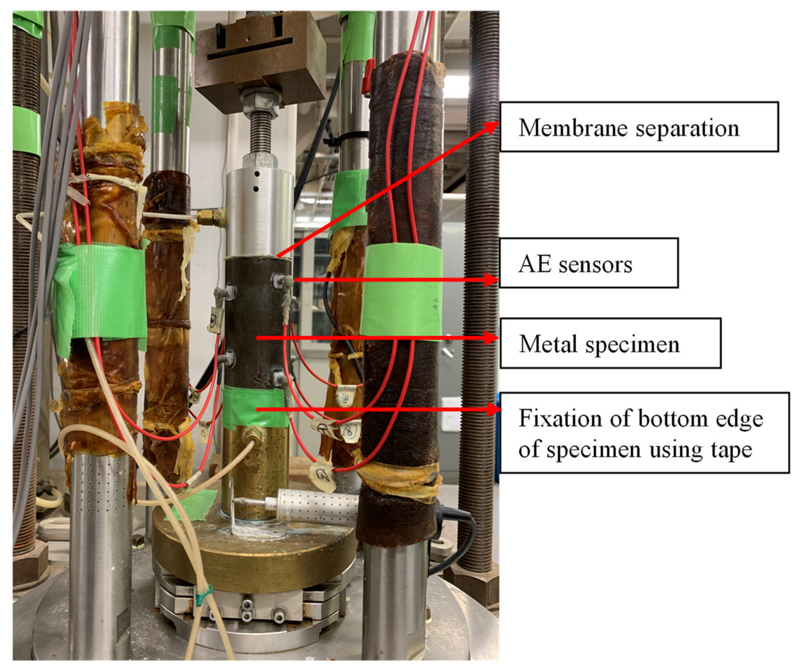
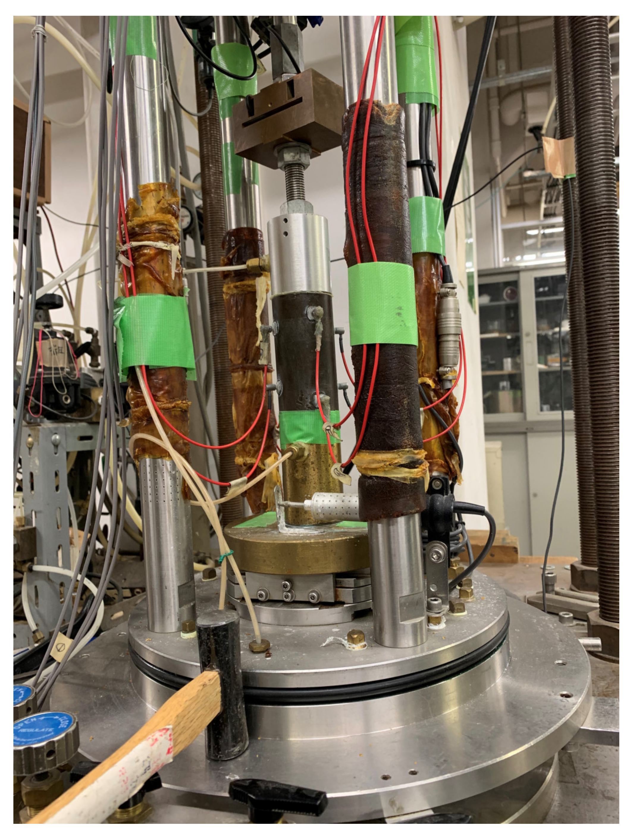
2.1. Set-Up

In this research, a traditional triaxial apparatus containing a motor-driven axial loading device was used. The specimen was a cylindrical metal specimen with the dimensions of 50 mm in diameter and 100 mm in height. It was made of S45C in Japan, which is a carbon steel for machine structures with a carbon content around 0.450%. To reduce the attenuation of waves, five sheets of 0.3 mm thick membranes were put in-between the top cap and the top surface of the specimen. The bottom of the specimen was connected to the pedestal directly using tape to fix the specimen and prevent movement, as shown in Figure 1. The verification test was performed under a static state without any loading.
Eight AE sensors were attached to the surface of the specimen with a small metal paste and glue (Figure 1). They were piezo-ceramic type M304A sensors with an operating frequency range of 10 kHz–2 MHz (the resonant frequency was 300 kHz), manufactured by Fuji Ceramics Corporation, with a sensitivity of 115 ± 3 dB (ref. 0 dB = 1 V/m/s). The origin coordinate is indicated in the Figure 2, and the location of the eight AE sensors is shown in Table 1.
The AE measurement system comprised the AE sensors, pre-amplifier, data logger, and a system for recording and analysis, as shown in Figure 3. The original AE signal was continuously recorded by the data logger, an NI PXIe-6366, with a sampling rate of 2 MS/s. The data logger and AE sensors are commercially available. Only the analysis system is original. A similar AE measurement system, especially the analysis component, was developed by Mao et al. [10] and improved by Lin et al. [11], which will be introduced briefly in Section 3.1. In Figure 3, stressed sands refer to sand specimens under triaxial compression loading. Here, one pencil lead break is expected to be used to simulate one AE source from the stressed sands in the triaxial tests, such as particle-to-particle sliding or particle crushing.

2.2. Experimental Method

2.2.1. PLB Tests

According to the ASTM E1316-14e standard [1], verification of the AE source location technique can be achieved by breaking a 0.5 mm HB pencil with a lead with a length of around 2.5 mm on the surface of the metal specimen. In general, the pencil lead breaks can be used to simulate the real crack formation and AE phenomenon. The PLB sources will propagate through the metal specimen and will be received by the AE sensors. In this study, the cylindrical side of the specimen was divided into four areas, which were the front, back, left, and right, as indicated in Figure 2. The pencil lead was broken three times at three different points (A–C, as shown in Figure 2) on each area of the specimen. Therefore, there were 36 PLB sources in total.

2.2.2. Noise Check Test

Considering the effect of outside noises from walking, speaking, working machines, and so on, a hammer hit is used to generate an enlarged noise outside the specimen, which was expected to have some obvious effect on the calculated result. The hammer hit position was decided at the point (0, 0.180, −0.180) in the 3D space, which was far from the specimen, as shown in the Figure 4. At the beginning, the noise check test was conducted three times using only the hammer hit. Then, a hammer hit source at the point (0, 0.180, −0.180) and a PLB source at B point were generated simultaneously to check the effect of outside noises on the calculated result directly. This test was also conducted three times.
The location of all PLB sources (36 without hammer and 3 with hammer, 39 in total) is provided in Table 2, along with the distances between the pre-set PLB sources and the coordinate origin, denoted as d0.

3. Principle of the AE Source Location Technique

3.1. Time Difference of Arrival (TDOA)

The AE source location technique employed in this study has been documented by Mao et al. [10], Lin et al. [11], and Li et al. [12] in detail. It is analogous to the back analysis of an earthquake epicenter. Based on the principle of TDOA, the location and the generation time of the AE source can be computed. According to Kundu [13], the travel distance between the AE source and the i-th sensor can be obtained by Equation (1) given below:
d i = t i t × v = x x i 2 + y y i 2 + z z i 2
where di is the distance between AE signal source and the i-th sensor;
t is the generation time;
ti is detected arrival time at the i-th AE sensor;
v is the AE wave velocity;
(x, y, and z) are the location of AE source;
(xi, yi, and zi) are the location of i-th AE sensor.
If one AE source is obtained by four AE sensors (e.g., No. S1 to No. S4), Equation (1) can be rewritten as Equation (2) given below:
f 1 = x x 1 2 + y y 1 2 + z z 1 2 t t 1 2 v 2 = 0 f 2 = x x 2 2 + y y 2 2 + z z 2 2 t t 2 2 v 2 = 0 f 3 = x x 3 2 + y y 3 2 + z z 3 2 t t 3 2 v 2 = 0 f 4 = x x 4 2 + y y 4 2 + z z 4 2 t t 4 2 v 2 = 0
The location of the sensors can be obtained from Table 1, and the wave velocity is assumed to be a constant value for a fully saturated sand specimen, as suggested by Lin et al. [11]. To verify the accuracy, a steel metal specimen was used in this study because of its lower attenuation property. Thus, the unknown generation time (t) and the location of the AE source (x, y, and z) can be calculated by solving Equation (2). Theoretically, it is possible to locate an AE source by using four AE sensors. However, in practice, more sensors are used to reduce the effects of potential errors, such as those of the positions of the attached sensors.
Regarding the detected arrival time, an automatic arrival time determination algorithm was developed by Mao et al. [10] based on the autoregressive-Akaike information criteria (AR-AIC, Akaike [14]). Further details of this algorithm are presented in Mao et al. [10] and Lin et al. [11].
Four channels were selected randomly to solve Equation (2) by the Newton–Raphson method [15]. Finally, using the least-squares method (LSM), the optimal solution from the smallest sum, S, can be picked up as Equation (3) given below:
S = i = 1 N x x i 2 + y y i 2 + z z i 2 t t i 2 v 2 2
Thus, the critical condition is that, when the sum of the squared difference of the distance between the calculated event and the candidate AE source is the minimum, the calculated AE source is regarded as the position where the AE event occurred.

3.2. P-wave Velocity Measurement for a Metal Specimen

For P-wave velocity measurement, the PLB test was conducted three times above AE sensor No. S3 along the line of No. S3 and No. S7, as shown in Figure 2. The arrival time was also obtained from the above-mentioned AR-AIC method. Then, the velocity of the metal specimen could be computed by Equation (4),
v = z 3 z 7 t 7 t 3  
where, z3 and z7 are the z coordinates of AE sensors No. S3 and No. S7, t3 and t7 are the detected arrival times at AE sensors No. S3 and No. S7, and v is the P-wave velocity of sound in metal specimen.
Finally, the average velocity of sound in the metal specimen was computed to be 5882 m/s, which is consistent with that the velocity of sound in steel metal, which is around 5556 m/s [16].

4. Results

Figure 5 presents the location of the calculated AE sources and the pre-set PLB sources in all tests. The black circles stand for the pre-set PLB sources. The red hexagons show the results on A point, the green ones show B point, and the blue ones show C point. The pink color is for noise check results. The shape ‘x’ identifies the calculated results with larger errors, which are inaccurate. In this study, any result (x, y, z, or d value) with errors greater than 30% was regarded as an inaccurate result. It was found that the green results are almost all around the pre-set B point, while the red results tend to be lower than the pre-set A point and the blue results tend to be higher than the pre-set C point. A more detailed analysis of the results will be introduced in the following sections.

4.1. Analysis Method and Results

As an index showing the accuracy of the analysis method, absolute error, which is the difference between the calculated and the pre-set value, was used to plot the frequency count histogram with a cumulative percent series. Additionally, the percent errors of generation time, the coordinate (x, y, and z), and the distance, d, were used to evaluate the accuracy of the AE source location technique through the following equations,
t _ e r r o r = t t 0 t 0 × 100 %
x _ e r r o r = x x 0 x 0 × 100 %
y _ e r r o r = y y 0 y 0 × 100 %
z _ e r r o r = z z 0 z 0 × 100 %  
d = x 2 + y 2 + z 2
d 0 = x 0 2 + y 0 2 + z 0 2
d _ e r r o r = d d 0 d 0 × 100 %
where t0 and t are the recorded trigger time and the calculated generation time, respectively; x0, y0, and z0 are the locations of the pre-set PLB sources as, shown in Table 2; x, y, and z are the locations of the calculated PLB sources; d0 and d are the pre-set and calculated distance from the coordinate origin, respectively; and t_error, x_error, y_error, z_error, and d_error are the percent errors of generation time, location, and distance, respectively.
According to the analysis method, the results are shown in Figure 6a–i. Figure 6a shows the percent error of generation time. It was found that all results of generation time were within an error of 7% and around 95% of them are within an error of 5%, which suggests that the calculated generation time has a good accuracy in this AE source location technique.
From Figure 6b–i, the absolute error and the percent error of the coordinates (x, y, and z) and the distance from the origin are presented. For the distance, d, as shown in Figure 6h,i, except for several points with a large error, around 90% of the PLB sources were within an absolute error of ± 15 mm and a percent error of ±10%. This is in good agreement with the study conducted by Lin et al. [11]. Thus, the existing AE source location technique is believed to be reliable, according to the generation time and the distance. For the specified coordinates along the x, y, and z axes, more than 90% of the PLB sources along the x and z axes were within an absolute error of ±15 mm, while along y axis, around 80% of the sources were within ±15 mm. Regarding the percent error, most of them were within ±30%. Thus, the existing AE method is proven to have the least error for the distance from the coordinate origin, with some errors along the x, y, and z axes. This suggests that the existing AE source location technique still needs further improvement.
For the z position, as shown in Figure 6f,g, it was found that the results on A point, marked as red columns, were within an error of ±10%. Most of them were negative, which means that the calculated result was lower than the pre-set PLB source. The results on B point, marked as black columns, were around the line of 0 percent error, suggesting that there was a higher accuracy around B point, with an error lower than ±5%. The results on C point, marked as blue columns, were positive, with a larger error of up to 30%, which means that the calculated result was higher than the pre-set PLB source. Thus, it seems that the calculated AE sources tended to be concentrated on the central part, with some errors, which is also mentioned in the pile model test by Hamaguchi et al. [17]. In their research, the accuracy of AE source location technique was higher around the center and became lower with the increase of the distance from the center.
In order to reflect real conditions, the triaxial loading tests were conducted, and their AE source location results were compared with an image analysis based on the particle tracking velocimetry from the front view in the first author’s PhD thesis [18]. It was found that the calculated AE sources tended to be concentrated on the central part, with some biases. Thus, the current research is a confirmation of the previously obtained results.

4.2. Noise Check Test Results

Regarding the noise check test, when the test was only conducted using a hammer hit, there was no AE source result, while there was a clear waveform change. On the other hand, when the pencil lead break and a hammer hit were applied at the same time, the results had almost no change, with an error of less than ± 5% (y and z axes and d), which is presented using pink in Figure 5a. Thus, a hammer hit noise, more than twice the height of the specimen away from the original point, has virtually no influence on this AE source location technique. Even such an enlarged noise, a hammer hit, had no effect on the calculated results. Those smaller noises (walking, speaking, and so on) far from the specimen should also have no effect on this AE source location technique.
For the inaccurate result of noise check test, the relevant percent errors were a y_error of −93.4%, z_error of −23.0%, the distance d_error of −25.0%, and t_error of 1.58%. Thus, it was possibly due to some technique error or human error. For example, when the pencil lead was broken, the source may have been too weak to be traced, by chance (e.g., the quality of pencil lead). However, after the pencil lead was broken, the mouth of the pencil may have touched the surface of the specimen by accident, which would affect the accuracy.
As mentioned previously, any result with a precent error more than 30% was considered to be inaccurate. According to Figure 5, there was 66.7% accuracy on A point and only 41.7% accuracy on C point, while there was 91.7% accuracy on B point (except in the noise check test). Thus, the calculated results on B point (the central part) had a higher accuracy than those results on A and C points. The calculated results on C point had a lower accuracy of 41.7%. This was possibly due to the direct connection of the metal specimen and the pedestal because it is easy for the PLB wave to be reflected through the connection surface of metal and pedestal. However, the membrane separation (Figure 1) in the upper side can help to reduce such attenuation and reflection of the PLB source wave. Thus, it is believed that the calculated results on A point are with higher accuracy (66.7%) than those results on C point (41.7%). This suggests that during the triaxial test, the connection of the specimen and pedestal/top cap would have some effect on the final calculation results. It should be noted that the authors just wanted to fix the specimen on the pedestal without considering such a problem in advance.
In fact, all the PLB sources were applied above the lowest sensors and below the highest sensors, meaning that the generated PLB sources were fully covered by eight sensors. Therefore, those PLB sources could reach the sensors directly, instead of reflections. However, following the results, such inaccurate results appear to be due to the different mounting of the upper part and the bottom part, which suggests that different mounting effects, such as reflections, exist. Moreover, in this real situation, the bottom side was connected to the porous stone and the pedestal and the upper side was connected to the porous stone and the top cap. They are also different connections; thus, they might have some influence on the calculated results. In the future study, a different method of mounting should be considered. So far, it is believed that if both sides have membrane separation, the accuracy of C point may be increased.

5. Conclusions

To verify the validity of the developed AE source location technique based on the time difference of arrival, pencil lead break tests have been conducted on a cylindrical metal specimen. In addition, the noise effect outside the specimen has been studied by using a hammer hit. The main conclusions that can be drawn include:
(a)
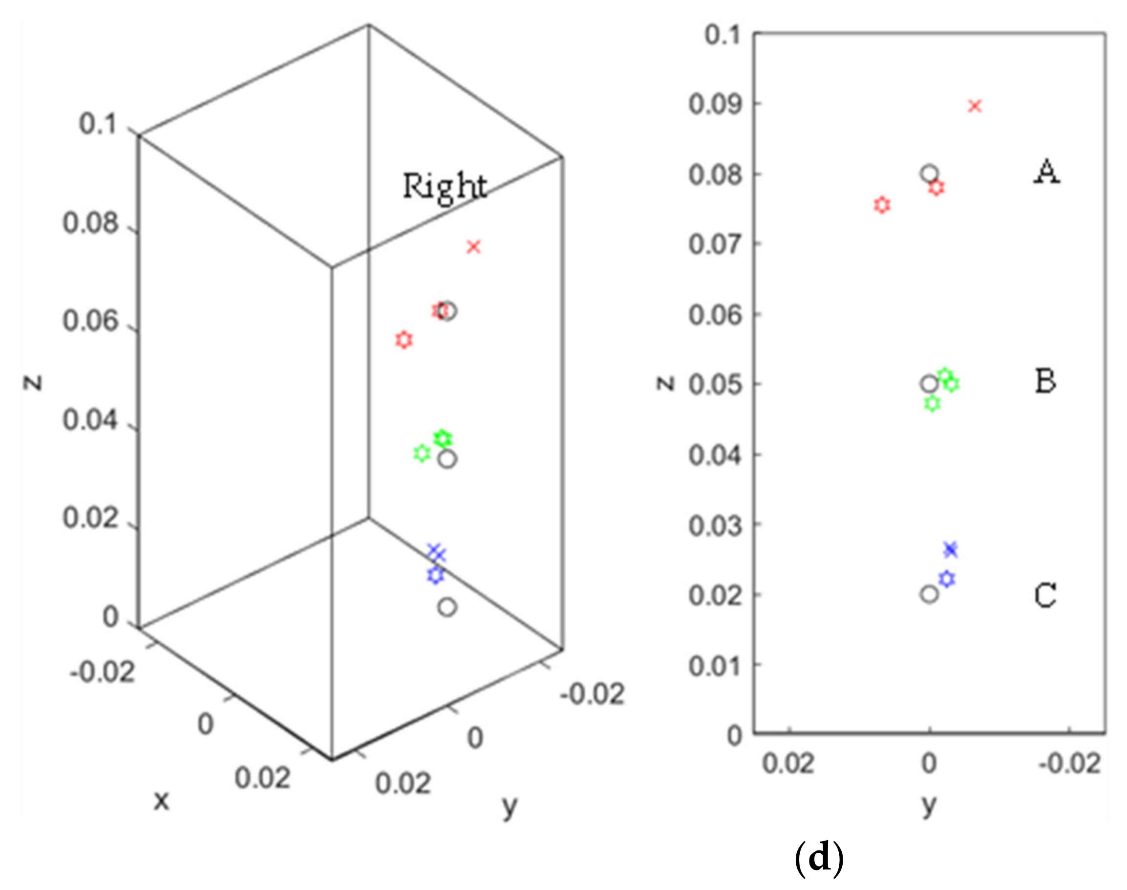
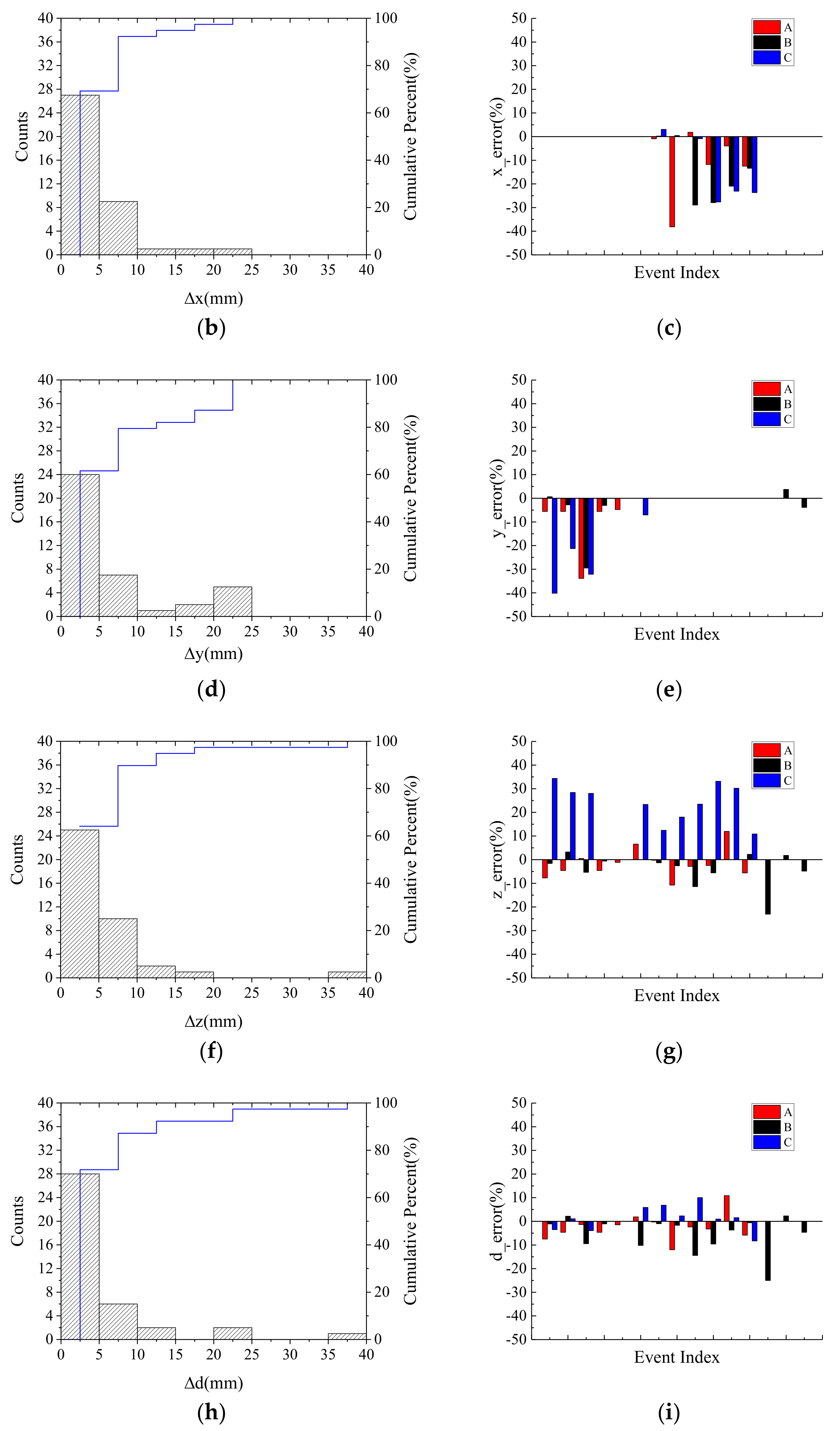
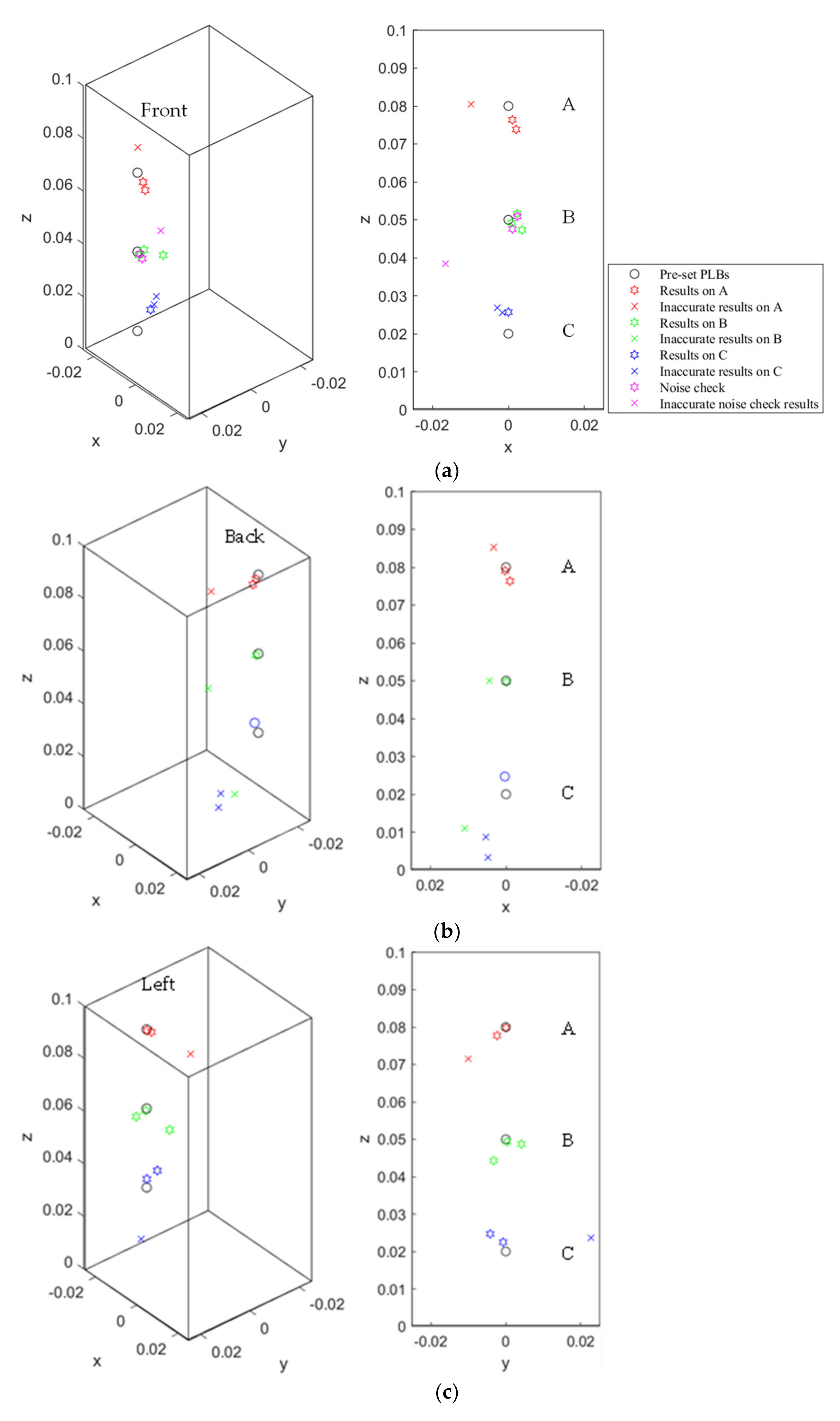
The validity of the developed AE source location technique was verified by PLB tests. The existing method was proven to have the least error in terms of distance from the coordinate origin but with some errors along the x, y, and z axes. When the PLB sources originate in the middle part of the specimen, the calculated result had higher accuracy, as compared to the other positions. Moreover, the calculated AE sources tended to be concentrated on the central part, with some errors.
(b)
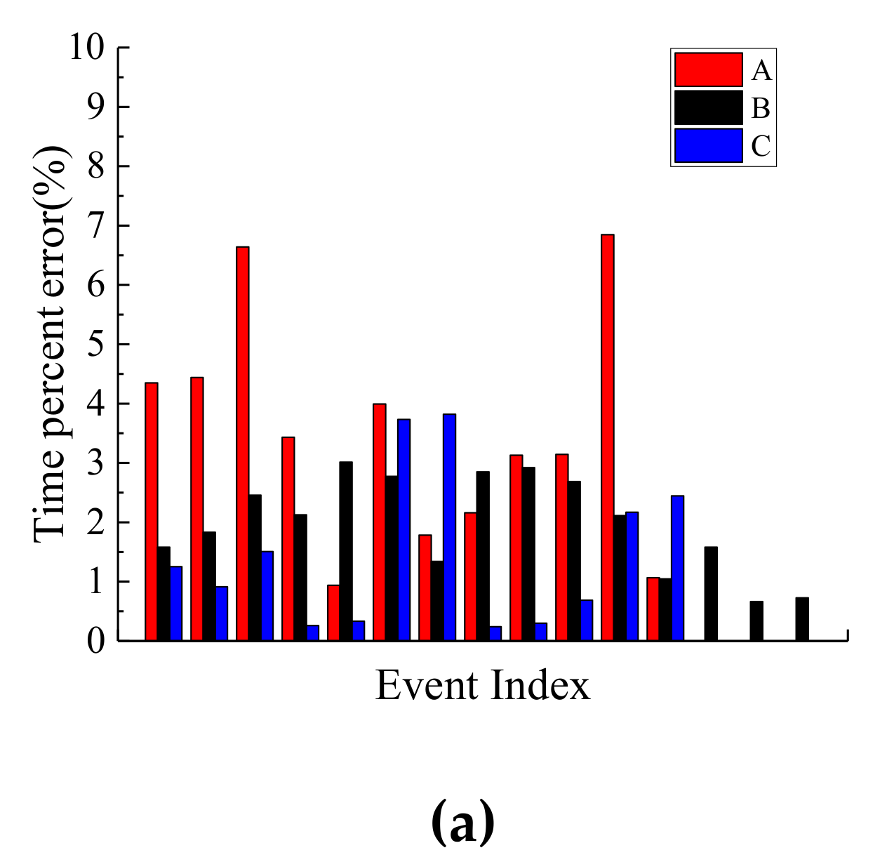
The outside man-made noise, i.e., a hammer hit noise, had virtually no effect on this AE source location technique.
In this study, the validity of the AE source location technique was verified by PLB tests on the metal specimen. However, in the triaxial tests, the AE sensors would move and even rotate because of shear banding failure or bugling failure. To solve this problem, the correction of the location of sensors is important, as mentioned by Lin et al. [11]. While in their research, it is still considered in a simple manner, the more accurate real-time location of AE sensors during the test is desirable. Another problem is how to determine an AE source (more detailed discussion will be published in the future). In the real case, especially for sandy soils, many AE sources could originate and arrive at the sensors almost at the same time. Thus, it is very difficult to determine an AE source. In this verification test, only one PLB source was made, without considering such a difficult problem. Therefore, the problem needs further study, for example, more verification tests can be conducted by using two, three, or even more PLB sources at the same time.
Only solving the above-mentioned problems will give a real answer as to the accuracy of the existing AE source location technique on sandy soils. Thus, the current research gives rise to further solutions, which could help to give a better understanding of the existing AE source location technique for sand specimens.

Author Contributions

Conceptualization, X.L. and J.K.; methodology, X.L. and A.N.; writing—original draft preparation, X.L.; writing—review and editing, A.N., Z.M., and J.K.; supervision, J.K. All authors have read and agreed to the published version of the manuscript.

Funding

Financial assistance for this paper was provided by the Japanese Ministry of Education, Culture, Sports, Science and Technology (MEXT, Grant No. 181534) and the China Scholarship Council (Grant No. 201706260011) for the PhD studies of the first author.

Institutional Review Board Statement

Not applicable.

Informed Consent Statement

Not applicable.

Data Availability Statement

The data are available from the authors upon reasonable request.

Acknowledgments

The authors would like to express their appreciation to Sato Takeshi and Liu Weichen of the University of Tokyo for their outstanding technical support and Mao Wuwei and Lin Wenli for their development and improvement of the AE source location technique at the University of Tokyo.

Conflicts of Interest

The authors declare no conflict of interest.

References

  1. ASTM E1316-14e; Standard terminology for nondestructive examinations. The American Society for Testing and Materials: West Conshohocken, PA, USA, 2015.
  2. Hasan, A.; Alshibli, K.A. Experimental assessment of 3D particle-to-particle interaction within sheared sand using synchrotron microtomography. Géotechnique 2010, 60, 369–379. [Google Scholar] [CrossRef]
  3. Koseki, J. Several challenges in advanced laboratory testing of geomaterials with emphasis on unconventional types of liquefaction tests. Geomech. Energy Environ. 2021, 27, 100157. [Google Scholar] [CrossRef]
  4. Mao, W.; Hei, L.; Yang, Y. Advances on the acoustic emission testing for monitoring of granular soils. Measurement 2021, 185, 110110. [Google Scholar] [CrossRef]
  5. Ohtsu, M.; Okamoto, T.; Yuyama, S. Moment tensor analysis of acoustic emission for cracking mechanisms in concrete. ACI Struct. J. 1998, 95, 87–95. [Google Scholar]
  6. Kurz, J.H.; Grosse, C.U.; Reinhardt, H.W. Strategies for reliable automatic onset time picking of acoustic emissions and of ultrasound signals in concrete. Ultrasonics 2005, 43, 538–546. [Google Scholar] [CrossRef] [PubMed]
  7. Shah, H.R.; Weiss, J. Quantifying shrinkage cracking in fiber reinforced concrete using the ring test. Mater. Struct. 2006, 39, 887–899. [Google Scholar] [CrossRef]
  8. Carpinteri, A.; Xu, J.; Lacidogna, G.; Manuello, A. Reliable onset time determination and source location of acoustic emissions in concrete structures. Cem. Concr. Compos. 2012, 34, 529–537. [Google Scholar] [CrossRef]
  9. Cadman, J.D.; Goodman, R.E. Landslide noise. Science 1967, 158, 1182–1184. [Google Scholar] [CrossRef] [PubMed]
  10. Mao, W.; Aoyama, S.; Towhata, I. A study on particle breakage behavior during pile penetration process using acoustic emission source location. Geosci. Front. 2020, 11, 413–427. [Google Scholar] [CrossRef]
  11. Lin, W.; Mao, W.; Liu, A.; Koseki, J. Application of an acoustic emission source-tracing method to visualise shear banding in granular materials. Géotechnique 2021, 71, 925–936. [Google Scholar] [CrossRef]
  12. Li, X.; Lin, W.; Mao, W.; Koseki, J. Acoustic emission source location of saturated dense coral sand in triaxial compression tests. Jpn. Geotech. Soc. Spec. Publ. 2020, 8, 331–334. [Google Scholar] [CrossRef]
  13. Kundu, T. Acoustic source localization. Ultrasonics 2014, 54, 25–38. [Google Scholar] [CrossRef] [PubMed]
  14. Akaike, H. Information theory and an extension of the maximum likelihood principle. In Proceedings of the 2nd International Symposium on Information Theory; Akademiai Kiado: Budapest, Hungary, 1973; pp. 267–287. [Google Scholar]
  15. Ben-Israel, A. A Newton-Raphson method for the solution of systems of equations. J. Math. Anal. Appl. 1966, 15, 243–252. [Google Scholar] [CrossRef] [Green Version]
  16. Zhukov, V.S.; Kuzmin, Y.O. The Influence of Fracturing of the Rocks and Model Materials on P-Wave Propagation Velocity: Experimental Studies. Izv. Phys. Solid Earth 2020, 56, 470–480. [Google Scholar] [CrossRef]
  17. Hamaguchi, H.; Mao, W.; Koseki, J. Model tests on application of AE tomography method to observe microscopic phenomena during pile penetration in sand. Jpn. Geotech. J. 2020, 15, 623–634. (In Japanese) [Google Scholar] [CrossRef]
  18. Li, X. Experimental Study on Acoustic Emission of Granular Materials under Triaxial Compression. Ph.D. Thesis, The University of Tokyo, Tokyo, Japan, 2021. [Google Scholar]
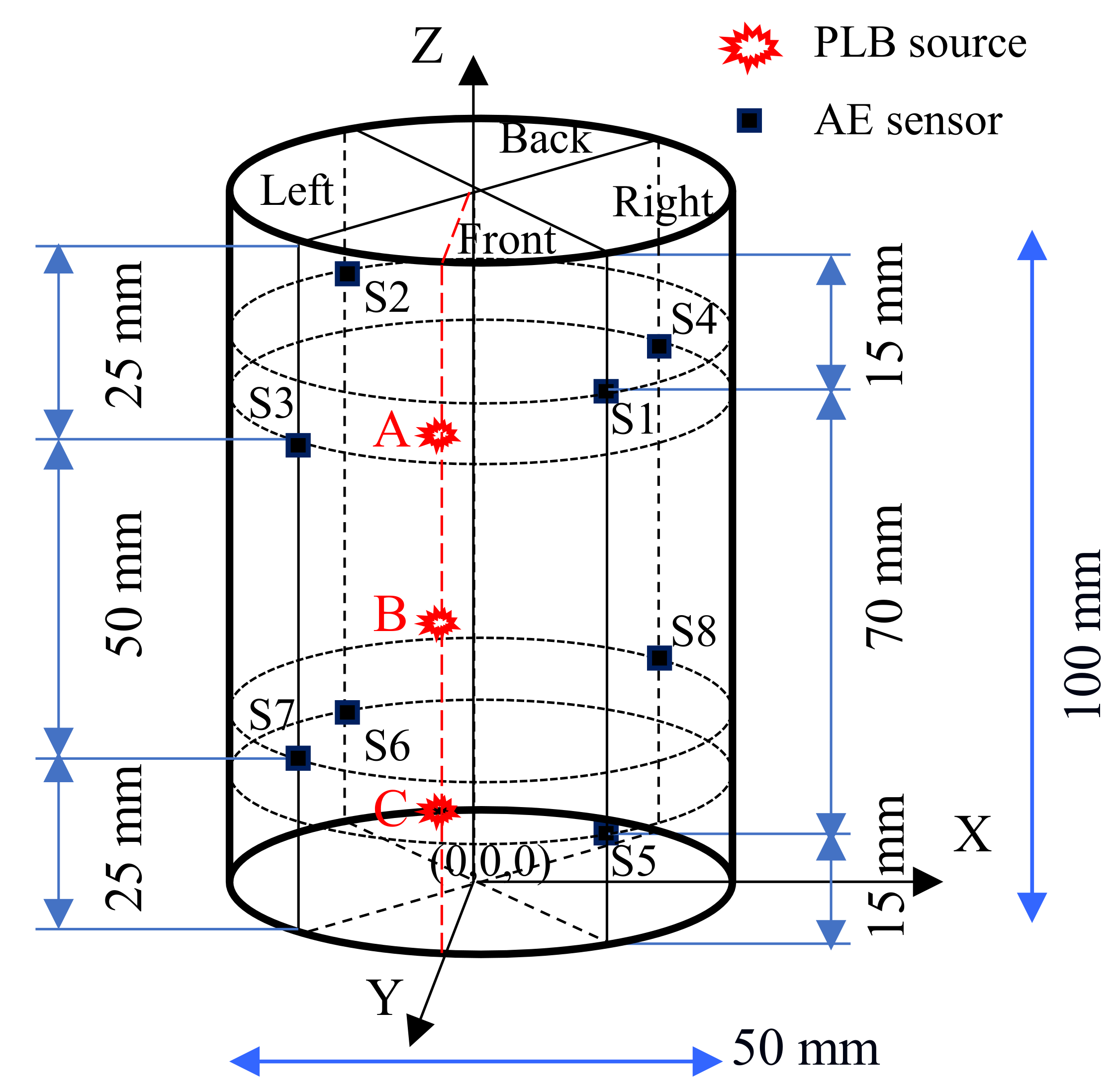
Figure 1. The specimen with eight AE sensors attached in the triaxial apparatus.
Applsci 12 01603 g001
Figure 2. Three-dimensional view of the specimen.
Applsci 12 01603 g002
Figure 3. AE measurement system.
Applsci 12 01603 g003
Figure 4. Man-made noise: a hammer hit.
Applsci 12 01603 g004
Figure 5. Comparison of pre-set PLB sources and the calculated AE sources in different views: (a) front view; (b) back view; (c) left view, and (d) right view.
Applsci 12 01603 g005aApplsci 12 01603 g005b
Figure 6. Evaluation of generation time, the coordinate (x, y, and z), and the distance from the coordinate origin: (a) Time percent error; (b) Frequency count histogram with a cumulative percent series and (c) the percent error along the x axis; (d) Frequency count histogram with a cumulative percent series and (e) the percent error along the y axis; (f) Frequency count histogram with a cumulative percent series and (g) the percent error along the z axis; (h) Frequency count histogram with a cumulative percent series and (i) the percent error, of the d value.
Applsci 12 01603 g006aApplsci 12 01603 g006b
Table 1. The location of the AE sensors in Cartesian coordinate system.
Sensor No.x/my/mz/m
S10.0180.0180.085
S2−0.018−0.0180.085
S3−0.0180.0180.075
S40.018−0.0180.075
S50.0180.0180.015
S6−0.018−0.0180.015
S7−0.0180.0180.025
S80.018−0.0180.025
Table 2. The location of all pencil lead break sources.
TestsLocationx0/my0/mz0/md0/m
PLB A0.0000.0250.0800.084
FrontB0.0000.0250.0500.056
C0.0000.0250.0200.032
A0.000−0.0250.0800.084
BackB0.000−0.0250.0500.056
C0.000−0.0250.0200.032
A−0.0250.0000.0800.084
LeftB−0.0250.0000.0500.056
C−0.0250.0000.0200.032
A0.0250.0000.0800.084
RightB0.0250.0000.0500.056
C0.0250.0000.0200.032
Noise checkFrontB0.0000.0250.0500.056
Publisher’s Note: MDPI stays neutral with regard to jurisdictional claims in published maps and institutional affiliations.

