Dynamic Discrete Inventory Control Model with Deterministic and Stochastic Demand in Pharmaceutical Distribution

Abstract

This paper presents an inventory control problem in a private pharmaceutical distribution company from the Republic of Serbia. The company realizes that distribution within nine neighbouring countries and inventory control in the pharmaceutical supply chain is centralized. In order to constitute a conceptual model of the problem, we propose the modern control theory concept. The conceptual model is based on the specific practical assumptions and constraints of the supply chain. Thereafter, a dynamic discrete mathematical model of inventory control is formulated to reflect elements of the system and their relations. The model considers multiple pharmaceutical products, variable lead time, realized stochastics and deterministic demand, and different ordering policies (Lot for Lot and Fixed Order Quantity). Deterministic demand is represented as a sales forecast for each product per month, while stochastic demand is generated as a random variation of sales forecast in a range of ±20%. Two objective functions are defined as the maximization of the difference between planned average inventory level and realized average inventory level, and the minimization of stock-out situations. We develop a procedure for the determination of reorder points and the number of deliveries to achieve proposed objective functions. The model overcomes shortages of theoretically-based distribution requirements planning models and offers solutions to the limitations in inventory control practice. Real-life data, collected over two years, are used for the validation of the proposed model and the solution procedure. Numerical examples illustrate the model application and behaviour.

1. Introduction

The importance of the pharmaceutical industry is directly associated with the fact that it deals with human life. Since the quality and security of pharmaceutical products must be constantly maintained, inventory management of the industry is quite a challenging job. According to [1], pharmaceutical companies handle approximately 500–600 types of products, and are responsible for a large quantity of unprocessed materials movement, packaging, secondary packaging of finished goods, and delivery to the customer. Inventory management of pharmaceutical products has become challenging for companies from health care industries, given that they continuously attempt to reduce costs and improve their customer service levels in a progressively competitive business environment [2]. Distribution management should ensure the delivery of required pharmaceuticals and inventory maintenance for facilities where they are needed, while costs of distribution should be the lowest. Distribution costs relate to storage, transport, customs and analysis, etc. The development of a model that enables effective control of storing and distribution of pharmaceuticals and medical supplies is important, but it is not a simple task. Pharmaceutical distribution effectiveness depends on the quality of control system design [3].

The topic of inventory control has been studied for many decades, within different business and scientific areas. Regardless of the implementation area, inventory control models are usually oriented toward cost reduction and maintaining appropriate inventory levels that satisfy customer demands and improve customer satisfaction [4]. Service level improvement is directly related to efficient management of the inventory level for each participant within the supply chain [5]. The importance of inventory holding and distribution in production and sale systems and their high associated costs are considered within numerous studies, aimed at examination and analysis of various models of inventory and distribution management [6,7,8,9].

Pharmaceutical supply chain (PSC) models are usually aimed at the optimization of specific unit operations, but according to [10], the implementation of theoretical approaches is often impossible due to complex dynamics of supply, distribution, and delivery systems. When it comes to mathematical models of PSC, papers are often oriented more on solving techniques than modelling itself (for example, [11]). Mathematical programming-type models of PSC are usually developed in order to optimize some figure of merit, for example in production-delivery system planning [12], strategic game-theoretic models of supply chain networks [13], and statistical frontier analysis models for supply chain management [14]. Although related to different categories, these types of models are based on a similar constrained optimization intent. PSC mathematical models should reflect current and alternative states of the modelled system (structural and behavioural characteristics) and enable their analytical evaluation, considering circumstances related to changes in market demands and resource availability [10]. A conceptual model of the modelled system should enable an overview of relevant facts for a mathematical model and actions that should be recognized as the identified solution. Furthermore, it is necessary to discuss the implementation of the models in real-world settings and the possible implications of such.

In order to overcome the described problems, we propose an integrated system approach, including problem conceptualization and the definition of boundaries, design, mathematical model formulation and solution, as well as the real-world implementation of identified solutions. A system of defining considers a combination of interacting discrete elements, which are organized in a manner that enables the achievement of the model purpose, which will be described within the paper.

The authors investigated a real-life inventory control problem in a private pharmaceutical distribution company, within a period of two years. The first, preliminary results were published in [15]. The final study, presented in this paper, extends the previous work in terms of methodology, mathematical model complexity, objective function, and practical applicability.

Aimed at the recognition of relevant elements that constitute the structure of the pharmaceutical distribution system in the real-world company, the authors of this paper propose the modern control theory concept for a conceptual model defining. Based on the defined conceptual model, a dynamic discrete mathematical model is formulated. The model implementation is realized in a spreadsheet, while practical evaluation is performed in the private pharmaceutical distribution company from the Republic of Serbia. The resulting dynamic discrete inventory control model is evaluated in the company Pharma 4U DOO, Serbia [16]. Some of the main characteristics of the proposed approach, compared to the related research analysed within the paper, are presented in

Table 1. Comparison of the proposed approach characteristics and related research.

Reference	Real-Life Problem Settings	Conceptual Model	Mathematical Model	Real-World Settings Implementation/ Practical Validation	Software Solution
[1]	No	No	Inventory management simulation model.	No	Arena simulation software
[2]	No	No	Inventory model that integrates continuous review with production and distribution for a supply chain involving a pharmaceutical company and a hospital supply chain.	No	MATLAB
[13]	No	Graphical representation of the supply chain network topology with outsourcing.	A supply chain network game theory model with product differentiation, outsourcing of production and distribution, and price and quality competition.	No	Not mentioned
[17]	The authors analysed data from a large urban hospital in order to model the patient demand process for Meropenem and proposed a nonstationary model for managing the drug.	No	A two-stage (multi-echelon) perishable inventory model	The model evaluation based on data from a large urban hospital that has over 350 inpatient beds and more than 14,000 adult admissions per year	Not mentioned
[18]	The study addresses the liquid pharmaceutical preparations inventory problem of a hospital.	No	A stochastic lead time inventory model for deteriorating drugs with fixed demand.	The authors used relevant data from a hospital in order to obtain the optimal reordering point, the optimal ordering lot sizes and optimal ordering cycle in weighting the shelf life of drugs and service level.	Not mentioned
[19]	Optimization of the sustainable humanitarian supply chain of blood products in Tehran.	A five-echelon blood supply chain network is presented that includes donors, mobile, fixed and regional blood collection centres, and hospitals.	A robust multi-echelon multi-objective mixed integer linear programming optimization model.	The application of the proposed model is investigated in a case problem in Tehran, where real data is utilized to design a network for emergency supply of blood during potential disasters.	The model is coded in GAMS and solved by CPLEX solver.
[20]	No, but the proposed sustainable distribution network model in pharmaceutical supply chain is customized for a real case study in Iran.	No	A multi-objective model fordesigning of a pharmaceutical distribution network according to the main concepts of sustainability i.e., economic, environmental and social.	The model is validated in the pharmaceutical distribution company in Iran, Darupakhsh Distribution Company.	Not mentioned
[21]	A systems thinking and modelling methodology was used to explore the functioning of the reverse logistics process in the Indian pharmaceutical industry, at a strategic level.	Based on System Dynamics.	No	Data collection was confined to stakeholders belonging to a PSC in the South Indian state of Kerala. The application of systems thinking and modelling was limited to the qualitative phases of the methodology.	Not mentioned
[22]	The considered case study is based on a comprehensive empirical study of nine different North European pharmaceutical companies.	A fully-specified case study research underpins the formulation of a mathematical model of the PSC.	A two-stage stochastic MILP model for addressing market launch planning in the pharmaceutical industry.	The model is applied to a case based on an empirical study. Only the market data has been generated through random sampling based on literature data.	OPL Studio 6.0
Current study	A real-life inventory control problem in a private pharmaceutical distribution company from the Republic of Serbia.	The modern control theory, System Dynamics and feedback control concepts based.	Dynamic discrete multi-echelon multi-product inventory control model.	Real-life data, collected over two years, are used for the validation of the proposed model and the solution procedure. The applicability of the model has been proven by its usage for procurement planning in the company within the period of two years. The created plan comprised more than 50 products per country for several countries from Eastern-Central Europe.	The model is implemented in a spreadsheet environment, and procedures are automated through Visual Basic for Application. It is affordable, but dynamic and flexible software solution, relatively easy to implement and use.

. Under the term approach, we consider a real-life problem conceptualization, the corresponding mathematical modelling, the model implementation in real-world settings, and the software solution choice. The related research comprised of papers dealing with the pharmaceutical supply chain and inventory management and related topics. Comparison criteria are chosen in accordance with the previously mentioned lack of PSC studies and requests defined by the company for which the inventory management solution was created.

Starting from this point, the paper is organized as follows. Section 2 presents an overview of related research, concerning multi-echelon pharmaceutical supply chain management, centralized or decentralized network design, distribution planning and control systems, with emphasis on the distribution requirements planning approach (DRP), fixed order quantity (FOQ) and lot for lot (LFL) lot-sizing rules. Additionally, this section tackles the novelty of the study against the existing literature in the field. Section 3 outlines the problem description, while the methodology including modern control theory concept used for the conceptual model definition, system dynamics modelling and discrete-time system control, is addressed in Section 4. The mathematical model, assumptions and notation are presented in Section 5. Section 6 refers to the model implementation and Section 5 to the sensitivity analysis and numerical results. Finally, the last section relates to the conclusions, a summary of all the above-mentioned content, and future work directions.

2. An Overview of Related Research

In this paper, we develop a centralized multi-echelon inventory control model for purchasing pharmaceutical products from a manufacturer and distributing them among multiple foreign markets under deterministic and stochastic demand. In the context of supply chain management, the echelon represents the physical location where the products are located [17]. A multi-echelon system is characterized by the connection of inventory decisions from downstream locations and upstream locations, such as, different markets and central warehouses or manufacturers [23], for example.

Multi-echelon inventory problems have been extensively studied for different applications. Nevertheless, most of the existing inventory models are not appropriate for pharmaceutical products. Pharmaceutical products are often more expensive than other products to purchase and distribute, while shortages cause a high cost related to wasted resources and preventable illness. Thus, inventory control of pharmaceutical products has to ensure high product availability, at the right time, at the right cost. Inadequate inventory management strategies in the pharmaceutical industry may have a significant impact on financial losses and people’s health. Consequently, inventory management of pharmaceutical products is more critical than for other products [2]. Based on the above-mentioned, a specific inventory model that reflects real-life problems is necessary for the control of pharmaceutical products, in order to maintain patients’ health and reduce unnecessary costs. Depending on the country, the procurement and distribution of pharmaceutical products can be organized regionally or in commercial supply systems, existing parallel with public systems. According to [3], considering national and regional levels, private distribution companies offer cost-effective alternatives for delivering and storing medicines.

From a supply chain network design point of view, a system can be either centralized or decentralized. The centralized system implies that all local warehouses deliver their demand information, like a forecasted demand, to a central warehouse or manufacturer. Aggregated demand, based on the received demand information, is used for the defining of the inventory control parameters in the central warehouse. When it comes to the decentralized system, local warehouses define inventory decisions independently. Schmitt et al. [24] suggest the centralization approach for deterministic supply and stochastic demand. In this case, the centralization results in a lower expected cost without affecting the variance of the cost compared to a decentralization approach. Enns and Suwanruji [25] state that centralized planning and control, characteristic for DRP, is beneficial under realistic situations of time-varying demand and replenishment time uncertainty. They examined performances of two common distribution planning and control systems, DRP and Order Point replenishment, within networks involving manufacturing, distribution and retail facilities. Results indicate that a centralized system performs best when demands vary through time and when there is significant uncertainty with respect to demand and replenishment times. The high performance is related to the ability of DRP to anticipate changes, based on forecast information, in demand along the supply chain and release time-phased orders in anticipation of future requirements. DRP and Order Point replenishment strategies require very different information. According to [25], complex and extensive software information systems are necessary for DRP systems. This is explained by the various nodes in the supply chain or distribution network that must communicate with the central planning function. Additionally, this constraint is important when the network nodes are controlled by independent enterprises. Intelligent information sharing in supply networks is analysed in [26]. Order Point systems require less coordination of information. The system implementation is much easier if it uses only inventory and order information local to the upstream replenishment loop.

Since this paper deals with the inventory control problem in the private pharmaceutical distribution company characterized by the transparency of information within the distribution network, we will review the DRP approach. According to [25], DRP is a time-phased replenishment approach, with inventory level monitoring and periodically realized delivery plans. In order to foresee requirements, companies use forecasting. Orders are realized, in accordance with inventory status and lead times, in a manner that minimizes inventory cost and, at the same time, prevents unnecessary shortages. The DRP system implies planned lead times and defined lot sizes. The fixed order quantity (FOQ) and lot-for-lot (LFL) lot-sizing rules, considered in this paper, are often used because they apply to each of the planning and control systems. FOQ and LFL ordering policy systems belong to a group of classical static inventory models. Some of the main assumptions of the model indicate the known total deterministic demand and order quantity that should be determined in a manner that minimizes stock-outs and the average level of inventories. As can be seen in [4,27,28,29,30,31,32], these classical inventory control models and their variations represent a starting point for understanding inventory dynamics, even in new books related to inventory control.

The mentioned DRP logic can be analogous with material requirements planning (MRP) logic, where forecasts are made based on customer demand (often a retail echelon). Planning of the orders in this manner is similar to order realizing for independent demand items in accordance with an MRP concept. A detailed comparison of MRP and production and inventory control theory, including their similarities and differences, is described in [33]. According to [33], unlike MRP logic, the inventory control approach includes forecasting and up-to-date re-planning based on system state changes. MRP reflects real-world planning, but decision-making procedure becomes difficult after incorporation of real-life constraints, while inventory control systems incorporate the presumption of real-life decision-making. Production inventory systems are often characterized by the uncertainty of external demand. MRP is applicable when future demands are known, on the contrary of production inventory control model defined by known inputs, previous actions and rescheduling. Grubbström et al. [33] proposed the integration of MRP, production, and inventory control logic in order to overcome their main disadvantages. Similarly, the authors of this paper propose the inter-linking of DRP and the modern control theory concepts aimed at the constitution of dynamic discrete inventory control models of the pharmaceutical distribution system in the real-world company. Some of the main disadvantages of the dynamic DRP model, which imply its improvement in order to solve the inventory control problem considered in this paper, can be defined as [25]:

• DRP does not determine the lot size or safety stock. These decisions represent inputs to the process;
• DRP does not explicitly consider any costs. These costs are still relevant because a user must evaluate costs of delivery;
• DRP systems cannot recalculate forecast if demand is changed in real-time (stochastic demand).

Inventory management of pharmaceutical products represents a ubiquitous topic in theory and practice. Consequently, there are numerous overview papers of high quality dealing with the subject. For example, [10,34,35] and many others. However, despite various studies, inventory control is still a daily burning issue for pharmaceutical companies. The implementation of different optimization models is often impossible in real-world settings. A possible solution implies a conceptual model of a system that enables an overview of relevant facts for a mathematical model and actions that should be recognized as the identified solution [10]. The aim of this paper is not the comparison of and with different approaches to pharmaceutical inventory control, and thus we will not further analyse related papers. This paper represents a real-life inventory control problem in a private pharmaceutical distribution company. The authors studied the problem within two years and noticed specific practical assumptions and constraints of the supply chain in the company. Another important request, defined by the company, was a software solution that is affordable, but dynamic, flexible, and relatively easy to implement and use. To the best of the authors’ knowledge, there is no research in the literature that has developed an inventory control solution appropriate to the identified characteristics of the problem, specific practical assumptions, constraints, and the company’s requests. This comprises:

• a centralized multi-echelon multi-product inventory control system with transparency of information within the distribution network, but without the necessary software information systems;
• nine regional pharmaceutical markets should be managed by a centralized inventory control model in PSC;
• the products should be distributed directly from the manufacturer to the customers because the distribution company does not store items in the main branch;
• a different FOQ or LFL order quantity should be considered for each product;
• a lead time (LT) is variable (approximately five months) and different for each product;
• an inventory plan is based on a monthly sales forecast for three months after the lead time period expiration and realized stochastic demand;
• shortages are allowed but not backlogged;
• two objective functions should be considered, the maximization of the difference between the planned average inventory level and the realized average inventory level and the minimization of the stock-out situations;
• the software solution should be affordable, but dynamic, flexible, and relatively easy to implement and use.

Additionally, we propose the conceptual model, which reflects the specificities of the system that are necessary for the mathematical model’s development. The conceptual model is in accordance with the modern control theory; consequently, the system is based on feedback control. The modern control theory concept and its implementation are described further in the paper, as is a discrete-time system control used for the system dynamics modelling.

3. Problem Description

4U Pharma GMBH is a Swiss company that produces and sells the highest quality natural pharmaceutical products, mainly for newborns, infants, and children [16]. The company production is grounded on the expertise and the knowledge of medical and herbal sciences of world-recognized scientists who are taking part in the creation and development of products. The company uses advanced and innovative technologies, combined with ingredients of the highest quality. Testing of the products is realized during every phase through clinical studies in order to confirm their efficacy in preventing and treating diseases. The head office of 4U Pharma is located in Switzerland. It is responsible for financial investments, technical, technological, and medical developments of products, and control of the financial operations of the company. There are registered subsidiaries in some markets, which are owned by the Swiss company, and in other markets 4U Pharma conducts its business operations through its partners or distributors. The products of 4U Pharma are registered and sold in twelve countries in Europe. In all counties in which it operates, the company is a credible partner of the national pediatric associations and neonatology associations. 4U Pharma products are recommended in all countries by local authorities and relevant government bodies, such as the ministry of health. Furthermore, in most countries, the products have become part of the national recommendations of neonatology associations, pediatric associations, ministries of health, as well as expert groups.

A branch in Serbia is the company Pharma 4U DOO [16], established for pharmaceutical distribution in the Balkan and neighbouring countries. The distribution company supplies wholesalers and pharmacies from Bulgaria, Rumania, Serbia, Croatia, Macedonia, Montenegro, Slovenia, Bosnia and Herzegovina, and Albania. Inventory management is very important for the company and represents its core activity. The inventory control problem, analysed in this paper, is related to the determination of order quantities and reorder points and the improvement of overall ordering policy concerning stock-outs, the average level of inventories, the number of orders, and costs. The specifics of the inventory problem solution, required by the company, consider the assumptions listed at the end of the previous section.

Based on the forecast and personal experience, the logistics manager of the company defines a sales plan for the next year at the end of the current year. The forecast refers to historical data from previous years. During a year, the manager receives stock reports from all customers within the region at the beginning of each month. The supplier, i.e., production plant, defines the fixed order quantity for each product. The FOQ is used for the calculation of order quantities and periods in which the ordering will be realized. The FOQ is not unique for each product, and, consequently, the unit price is different for different order quantities. Product sales forecasts for all countries represent a base for the determination of order quantities. The defined order quantity should meet the demand per product for all countries. The company Pharma 4U DOO does not have warehouses in the Republic of Serbia. Products are distributed to customers directly, after customs and analysis. The process specificity is reflected through the long lead time of approximately five months (118–148 days). The total lead time consists of the production lead time (90–120 days), transportation lead time (up to 7 days), and custom and analysis (up to 21 days).

The ordering problem is defined for two instances related to FOQ and LFL ordering policy, respectively. Both instances imply maximization of the difference between the planned and the realized average inventory level, as well as minimization of the number of stock-out situations. In the case of FOQ ordering policy, the reorder quantities and reordering periods should be determined for each product for all countries, in a manner that provides enough inventories to satisfy the cumulative monthly sales forecast. LFL ordering policy refers to a moving horizon situation. The reorder quantities and reordering periods should provide enough inventories to cover the cumulative monthly sales forecast calculated for three months occurring after the lead time period expiration.

4. Methodology

The study presented in this paper considers a real-life inventory control problem detected in a private pharmaceutical distribution company. The study is realized over two years, from 2017–2019. As previously mentioned, the authors of the paper proposed a conceptual model based on the modern control theory concept and in accordance with the specific practical assumptions and constraints of the supply chain noticed in the company. Thereafter, a dynamic discrete mathematical model of inventory control is formulated in order to reflect elements of the system and their relations. Aimed at satisfying the company’s request, related to the affordable but dynamic and flexible software solution that is relatively easy to implement and use, the model is implemented in a spreadsheet environment, and procedures are automated through Visual Basic for Application (VBA). In order to evaluate the model’s performance, sensitivity analysis is performed for two instances related to the FOQ and LFL ordering policy. Validation of the proposed model and the solution procedure is realized in the company, for a few consecutive years, and based on real-world data.

The remainder of this chapter describes the mentioned concepts and approaches that were applied in order to solve the inventory control problem identified in the company Pharma 4U DOO.

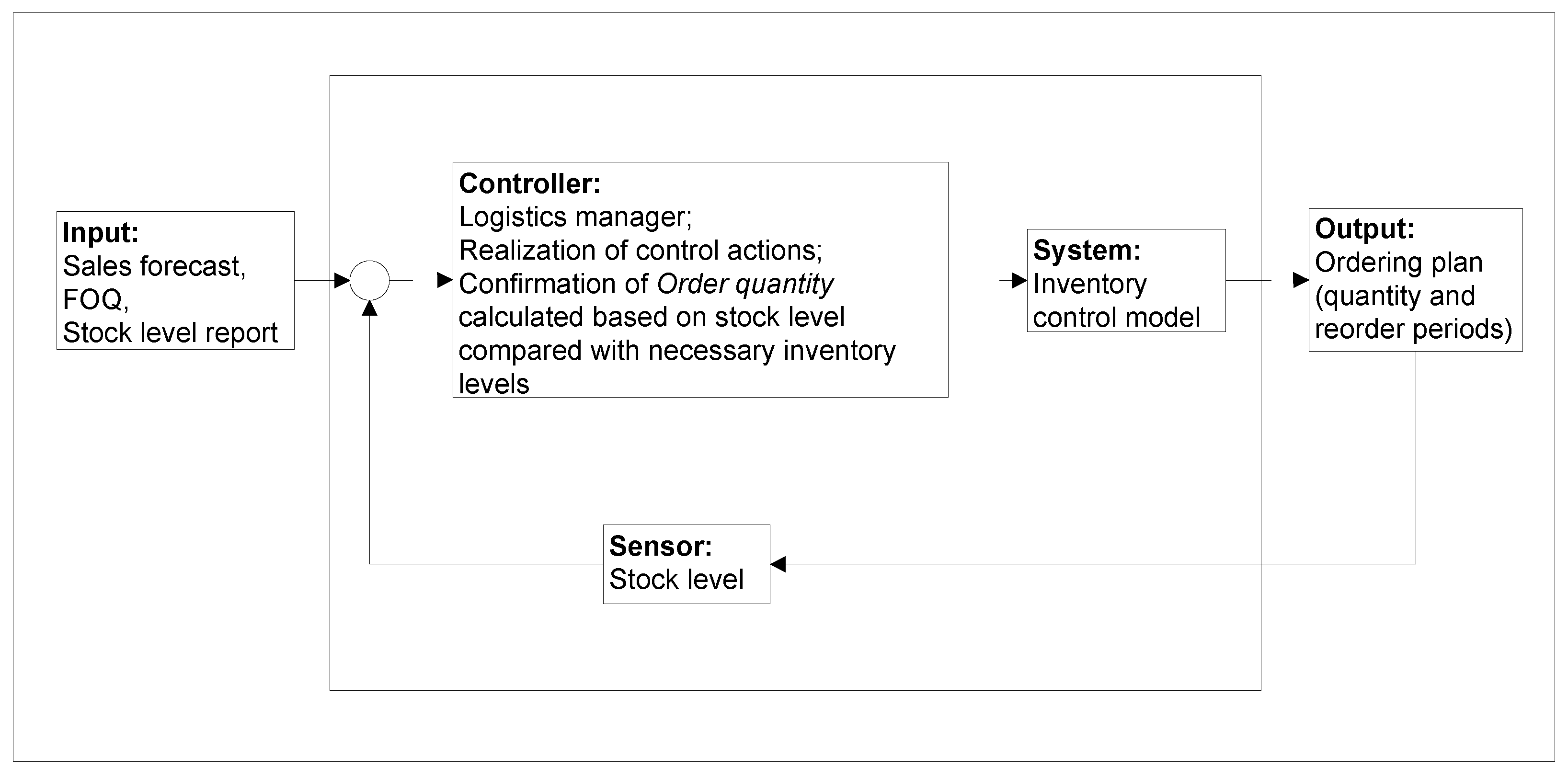
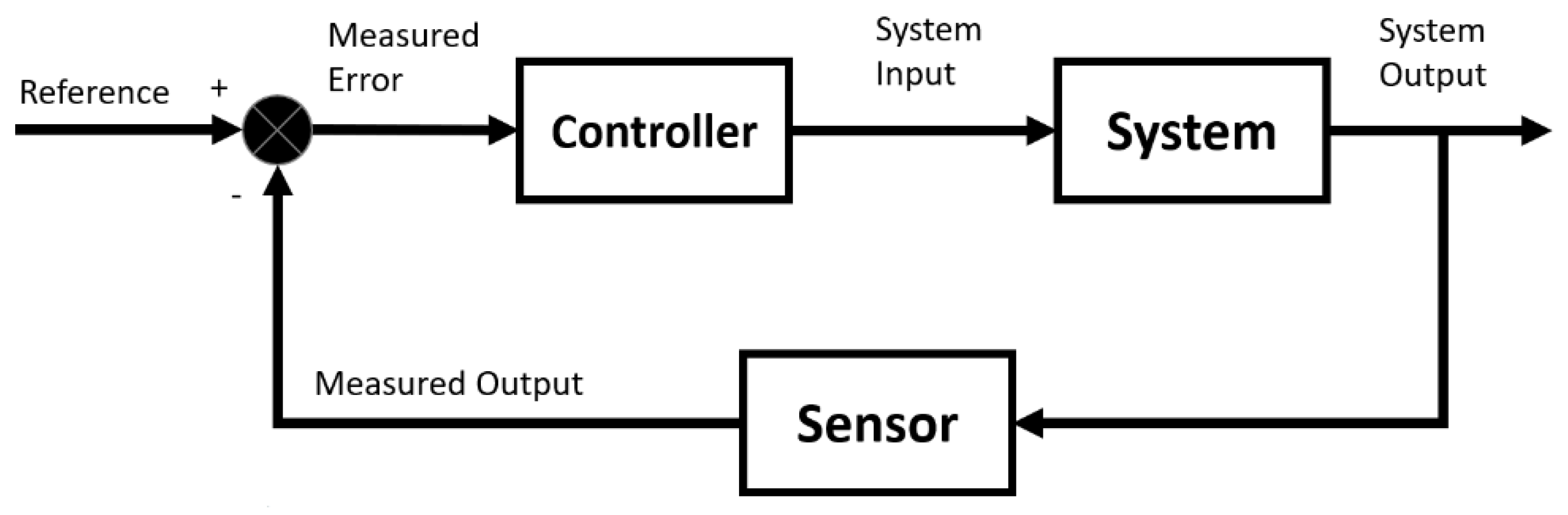
4.1. Modern Control Theory

A large number of natural laws, features, and capabilities of flora and fauna are used in the design of technical solutions. One of the main features of living systems and processes is self-regulation and feedback. For example, when the body’s temperature rises, the body begins to sweat in order to lower the body temperature. This reaction happens automatically and is enabled by the feedback of a self-regulation system. The concept of self-regulation and feedback could be used in the control of organizational systems. For example, a feedback control could be applied to developing a decision model for inventory control. According to [36], “The modern control theory (MCT) is a discipline dealing with formal foundations of analysis and design of computer control and management systems. The basic scope of MCT includes problems and methods of control algorithms design. The control algorithms are understood as formal prescriptions (formulas, procedures, programs) for the determination of control decisions. The control decisions may be executed by technical devices related to information processing and decision-making”. The importance of this area of application is indisputable. Contemporary business development, closely related to information systems and technology development, influences the expansion of MCT application areas. As stated in [36], automation of the control includes automation of manipulation operations, control of executing mechanisms, intelligent tools and robots, and inner control of devices and systems. Modern control science has developed in line with new needs related to the control of numerous technical processes in factories, but it also includes project management and computer systems control and management. Consequently, the scope of modern control science is much wider than the traditional control theory. The development directions of MCT comprise methods that improve the design and the usage of computer tools in the decision support systems. Control and management systems represent one of the largest classes of such systems [36]. A control system design typically implies many steps, described in [37].

One of the most common concepts related to control systems is a feedback loop. The system output represents the signal that should be controlled. Comparing this signal and the desired reference signal results in a gap used for computing corrective control action [38]. In accordance with [38], the most elementary feedback control system has four elements (Figure 1):

–

A system or plant (the object to be controlled);

–

A sensor (used for measuring the system’s output);

–

A comparator (used for comparison of the input or reference signal and the output signal converted by the sensor);

–

A controller (an element that generates the system’s input–control action).

The reference or planned value represents an external input of a system. As can be seen in Figure 1, a controller influences the inputs of a system in order to achieve the planned output value of a system. One of the main objectives of control theory is the determination of corrective action in the controller in order to obtain system stability. The focus of the feedback loop concept is to control the dynamic behaviour of the system over time. The error signal used in a controller is calculated by subtraction of the sensor value from the reference value. The sensor converts output of a system into a readable output, which can be compared with the reference value [38]. The measured output provides information to the control system related to the value under control, which should be regulated within some “set point” range. As explained in [39], the closed control loop refers to a situation in which the controller output corrects measured deviations from the set point.

Feedback represents a ubiquitous concept in various areas of activity. A feedback process is characterized by the state of the system or its output, which determines the manner in which the control has to be computed at any time instant [40]. Feedback systems are typical for both natural and engineered systems. The meaning of the control term depends on the application area. For the purpose of this paper, control is defined as the usage of algorithms and feedback in engineered systems [41]. The applicability of MCT for inventory control is presented in many papers [37,42,43,44].

As mentioned earlier, the inventory control problem modelling is based on the feedback loop principle. Elements of the feedback loop for the inventory control model are presented in Figure 2. A detailed explanation of the model elements is shown in [15] and in the following of the paper.

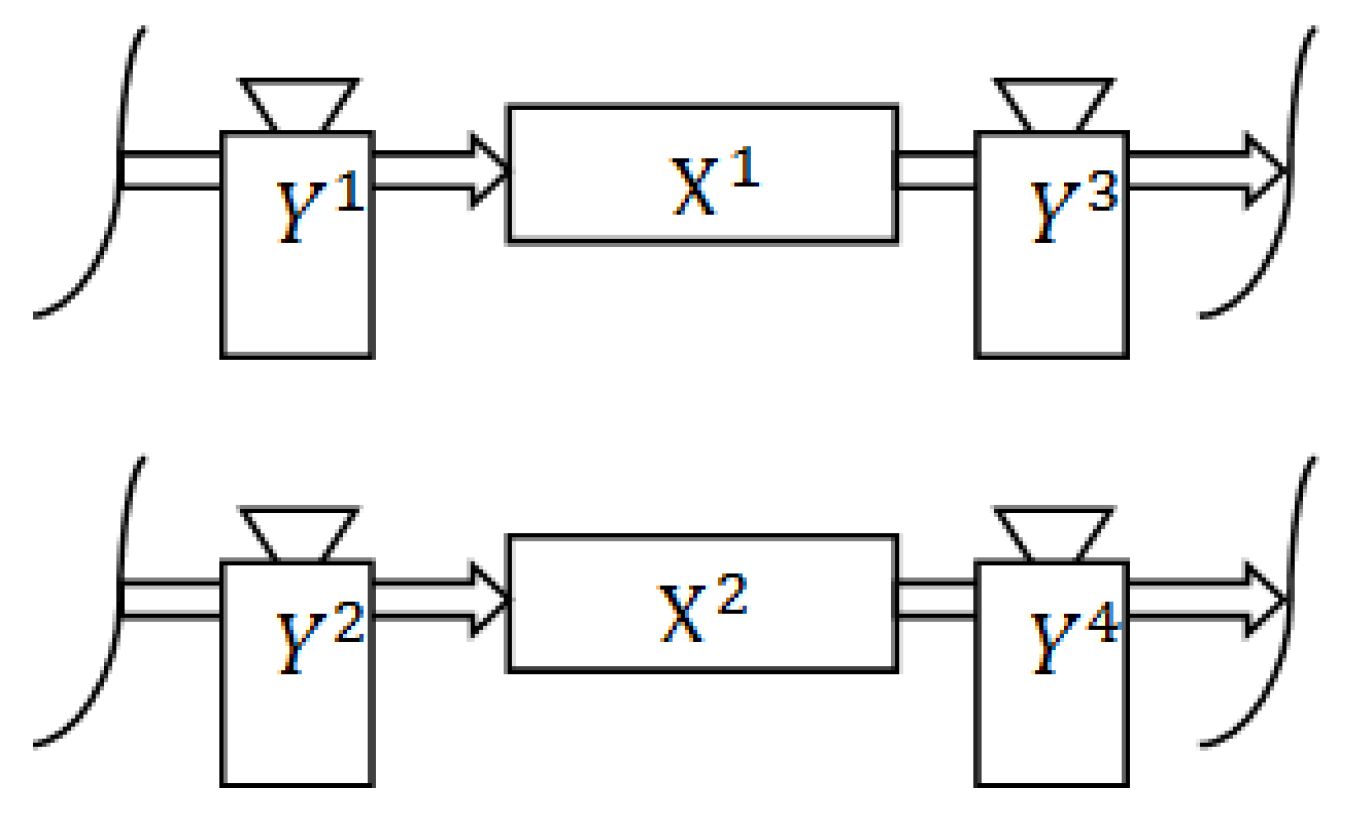
4.2. Discrete-Time System Control—System Dynamics Modelling

System dynamics (SD) is a modelling approach widely used in logistics and supply chain management [45]. System dynamics (SD) relates the modelling of processes over time. SD is often considered a modelling technique based on continuous time [46]. In this paper, we consider SD modelling also for the discrete concept of time. Finite changes over time mode means dealing with changes over time in a manner that resembles our everyday experience. It is based on a simple principle: “In order to notify some change, some time has to pass by” [46]. Changes are related to time intervals, whereas the state of a variable is specified for specific points of time. The distinction between time-points and time-intervals yields two distinct types of data: data related to time-points and data related to time-intervals. The data relating to time-points will be named stocks and the data related to time-intervals flows. If the stocks are considered as state variables for time-points and the flows as changes of the stocks for certain time-intervals, the relation between the stocks and the flows is trivial arithmetic. For a given time interval (t₀, t₁) and given flows for that time interval we can calculate the “new” value of the stock at the end of the time interval according to the following equation [46]:

stock(t₁) = stock(t₀) + inflows(t₀, t₁) − outflows(t₀, t₁)

A stock accumulates its flows. According to the stock-flow principle [46], the new stock(t) is defined through the initial stock(t₀) plus all inflow(s) subtracted by all the outflow(s) between the time t₀ and time t. The core idea of SD modelling is the accumulation of flows over finite time intervals of duration discrete time periods, t. On the stock-flow diagram, there are two main types of elements: flow regulators (actions) and stock as state variable (accumulations) [47].

The control model of the problem defined in this paper implies two flows (Figure 3), the information flow of the planned inventory state and the material flow of the actual state of inventory. Each flow has three phases, one phase of accumulation and two phases of action. The action phases represent input and output flow regulators, respectively. The accumulation, representing inventory level, for each flow, is calculated with the quantity of the inventory from the end of the previous time period and is increased by the planned or realized quantity for delivery over the observed period of time, and it is reduced by the planned or realized sales over the period of time. For example, Figure 3 shows the stock-flow diagram for one item (one stock keeping unit–SKU, t = 1 … 24 months). In order to define a discrete-time mathematical model of the problem, a notation will be defined per type of element of the system and from the position of the element on stock-flow diagram (from top to bottom, and from left to right). For the stock-flow diagram presented by Figure 3, the following notations will be used:

• $X_t^1$—State variable. Planned stock level of a product on hand at the end of period t.
• $X_t^2$—State variable. Realized stock level of a product on hand at the end of period t.
• $Y_t^1$—Inflow regulator variable (left upper). Planned stock input of a product at the beginning of period t.
• $Y_t^2$—Inflow regulator variable (left lower). Realized stock input of a product at the beginning of period t.
• $Y_t^3$—Outflow regulator variable (right upper). Forecasted sales plan for a product for period t.
• $Y_t^4$—Outflow regulator variable (right lower). Realized sales of a product at period t.

The regulator variables have the same notation Y, because of the same nature of the flow, but have different superscripts suitable for the writing of equations describing the system. Defined notation is used for the formulation of the control system model, for example:

$$\begin{gathered} X_t^1=X_{t-1}^1+Y_t^1-Y_t^3, t=\overline{1, 24} \\ {X}_t^2=X_{t-1}^2+Y_t^2-Y_t^4, t=\overline{1, 24} \end{gathered}$$

Or summarized as follows:

$$X_t^i=X_{t-1}^i+Y_t^i-Y_t^{i+2}, t=\overline{1, 24}, i=\overline{1,2}$$

In the following of the paper, the notation of variables is defined in the described manner, for two distinctive flows, the planned flow of stock and the realized flow of stock, for each SKU. Each flow implies the same elements: two regulators, and one state variable.

According to [47] a discrete-time system control, used for the system modelling, represents a natural manner for describing inventory dynamics. Many papers describe the usage of the discrete-time system control for dynamic deterministic inventory problems. Frequently, they consider lot-sizing problems, beginning with [48,49]. Solving proposals for dynamic lot-sizing problems include dynamic programming algorithms [50] and different special heuristics and metaheuristics [51,52]. The dynamic discrete-time system modelling approach is used for the inventory control system in this paper due to its wide applicability and many benefits. These models enable relatively simple and not time-consuming modifications in accordance with newly discovered facts about an observed problem by changing some of the discrete control object elements. For example, adjusted elements related to the objective function allow model variations or even the setting of a new model, without modifications of other model elements, such as the law of behaviour for state variables, flow regulators, and the control space. Definitions and implementation guidance for dynamic discrete inventory control models can be found in [47,53]. According to [47], relations of the law of dynamics and control domain determine a discrete controlled object. These relations also represent the simulation model of the controlled object. System state changes are observed at the end of the discrete period t (day, month, year, etc.) of a time horizon. Decisions made in one period of time influence states and, consequently, new decisions in future periods. The success of the control is measured for each period by a defined objective function. The performance criterion is an objective function that adds values throughout the time horizon [47].

5. Mathematical Formulation, Assumptions and Notation

The considered problem is represented as a dynamic discrete multiproduct inventory control model. This section represents the mathematical formulation of the model, along with notation and assumptions.

5.1. Assumptions

In addition to the assumptions described within the problem description, the inventory replenishment problem is modelled in accordance with the following assumptions:

• Lead time (LT) includes the time necessary for the delivery of goods from the manufacturer to the distributor. Delivery time includes time periods from ordering to receiving the goods.
• Shortages are allowed but not backlogged, i.e., stock-out situations should be minimized.
• The initial inventory level is known.
• Order quantity depends on the observed instance:

  ○

  Fixed, i.e., the manufacturer defines the fixed order quantity per each product, but periods between orders are not fixed.

  ○

  Lot-for-lot, i.e., cumulative monthly sales forecast for three months, in a moving horizon situation, after the lead time period is expired, but periods between orders are not fixed.

• The sales forecast is known and forecasted for two years.

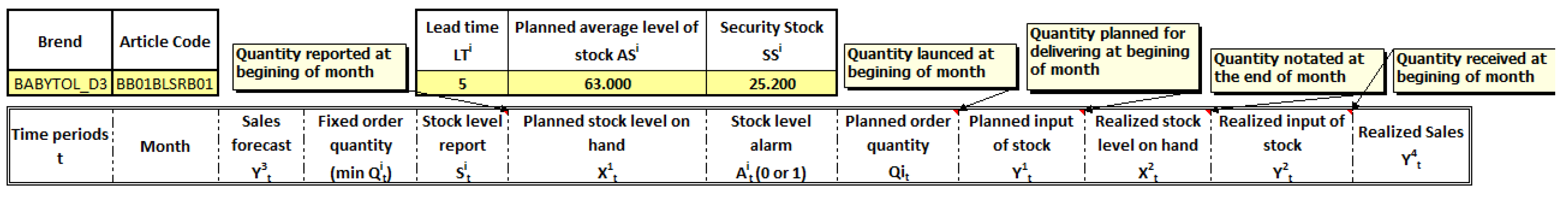
5.2. Notation

In order to explain the model, the following notations are used:

–

m–Total number of products ($i$ = 1, 2, …, m).

–

T–Finite time horizon T = 24 months (t = 1, 2, …, T).

–

LT–Delivery lead time.

–

$X_t^{i1}$–Planned stock level of product $i$ on hand at the end of period t. This phase of accumulation represents the total amount of product i remaining on the stock at the end of period t on the flow of the planned state of inventory $\left(t=\overline{1, 24}, i=\overline{1,m}\right)$.

–

$X_t^{i2}$–Realized stock level of product $i$ on hand at the end of period t. This phase of accumulation represents the total amount of product i remaining in the stock at the end of period t, on the flow of the realized state of inventory $\left(t=\overline{1, 24}, i=\overline{1,m}\right)$.

–

$Y_t^{i1}$–Planned stock input of product $i$ at the beginning of period t. This inflow regulator represents the amount of product $i$ expected to be delivered after the lead time at the beginning of period t. It is the regulator of the flow of the planned inventory state $\left(t=\overline{1, 24}, i=\overline{1,m}\right).$$Y_t^{i2}$–Realized stock input of product $i$ at the beginning of period t. The inflow regulator represents the input variable that relates to the inventory fulfilment at the beginning of the month. This flow regulator represents the amount of product $i$ delivered to the warehouse after the lead time expiry. It pertains to the flow of the realized state of inventory. The variable value is confirmed in the company’s software when order quantity arrives in the stock $\left(t=\overline{1, 24}, i=\overline{1,m}\right)$.

–

$Y_t^{i3}$–Forecasted sales plan for product $i$ for period t. This outflow regulator represents the amount of product $i$ planned for withdrawing from the accumulation of the planned inventory state continuously per month. The sales manager forecasts the sales plan for 24 months $\left(t=\overline{1, 24}, i=\overline{1,m}\right)$.

–

$Y_t^{i4}$–Realized sales of product $i$ at period t. This outflow regulator represents the amount of product $i$ actually withdrawn from the accumulation of the realized state of inventory continuously per month $\left(t=\overline{1, 24}, i=\overline{1,m}\right)$.

–

$\min Q_t^i$–FOQ for the product $i$ in period t, defined by manufacturer $\left(t=\overline{1, 24}, i=\overline{1,m}\right)$.

–

$L{Q}_t^i$–LFL order quantity for each product i $\left(t=\overline{1, 24}, i=\overline{1,m}\right)$.

–

$S_t^i$–The auxiliary variable representing value from a stock level report for product $i$ at the beginning of period t $\left(t=\overline{1, 24}, i=\overline{1,m}\right)$, and representing value obtained from stock level report, which is provided each month from a warehouse of a distributor. This variable presents an exact level of inventory for product i.

–

$A_t^i$–The auxiliary variable indicates if the planned stock level on hand $X_t^{i1}$ is greater than security stock $S{S}_t^i$ for product $i$ in period t $\left(t=\overline{1, 24}, i=\overline{1,m}\right)$.

–

$Q_t^i$–The planned re-order quantity for product $i$ in period t $\left(t=\overline{1, 24}, i=\overline{1,m}\right)$.

–

$S{S}_t^i$–The security stock for product $i$ in period t of time horizon T ($t=\overline{1, 24}, i=\overline{1,m})$.

–

$A{S}_t^i$–The planned average level of stock for product $i$ in period t of time horizon T ($t=\overline{1, 24}, i=\overline{1,m}$).

–

∆tⁱ–The auxiliary variable for calculation of the $L{Q}_t^i$ in the case of a lot-for-lot ordering policy ($i=\overline{1,m}$).

5.3. Mathematical Formulation of the Inventory Control Problem

The problem described in the above sections is considered as a time-continuous multiproduct inventory control problem. For each product $i$ the total deterministic demand should be satisfied within a finite time horizon T = 2 years (24 months) in the following manner:

• The same or variable amount $Q_t^i$ of product $i$, depending on the ordering policy, is ordered with no constant time t_i between the two orders.
• The ordered amount $Q_t^i$ arrives on the stock simultaneously and immediately after LT, while products are withdrawn from the stock continuously by the rate of the sales plan.

The problem is modelled as the corresponding discrete-time system control process. Rather than continuous time periods for products ordering, the entire time horizon $\left[0,T\right]$ is divided into n periods t with the same length $T/n$, where $t=1,\dots ,n$. For example, if T is a year then t is a month. Ordering of any product can be realized only at the beginning of a period t. During this period of length $T/n$ the products are withdrawn from the stock continuously in accordance with the sales plan $Y_t^{i3}$.

The decision variable $Q_t^i$ is generated in the model for all time periods. The inventory state of the product $i$ changes during the entire period of time. The inventory system can be formally represented as a discrete-time system control process with the following elements:$X_t^{i1}$, $X_t^{i2}$, $Y_t^{i1}$, $Y_t^{i2}$, $Y_t^{i3}$ and $Y_t^{i4}$. If we consider $X_t^{i1}$ and $X_t^{i2}$ as the state of a process at the end of each period t, then Equations (1)–(3) describe the low of behaviour of the discrete-time process, defined as follows. At the beginning of the time horizon, the initial inventory level is known and has to be a non-negative value (≥0).

$$X_0^{i1}=known, X_0^{i2}=known, i=1, 2,..., \mathrm{m}$$

(1)

Inventory dynamics of accumulation $X_t^{i1}$ are described by Equation (2) and appoint that the planned stock level of product $i$ on hand at the end of period t depends on the stock level of product $i$ at the end of the previous time period t − 1, increased by all inputs and decreased by all outputs during the time period t.

$$X_t^{i1}=\left\{\begin{array}{c}\left\{\begin{array}{c}\hspace{1em}0, X_{t-1}^{i1}+Y_t^{i1}-Y_t^{i3}<0\\ X_{t-1}^{i1}+Y_t^{i1}-Y_t^{i3}, otherwise\end{array}\right\}\\ S_t^i-Y_t^{i3}, otherwise\end{array}, S_t^i=0\right\}, t=\overline{1, 24}, i=\overline{1,m}$$

(2)

A similar Equation (3) is developed for the realized stock level of product $i$ on hand at the end of period t.

$$X_t^{i2}=\left\{\begin{array}{c}\left\{\begin{array}{c}\hspace{1em}0, X_{t-1}^{i2}+Y_t^{i2}-Y_t^{i4}<0\\ X_{t-1}^{i2}+Y_t^{i2}-Y_t^{i4}, otherwise\end{array}\right\}\\ S_t^i-Y_t^{i4}, otherwise\end{array}, S_t^i=0\right\}, t=\overline{1, 24}, i=\overline{1,m}$$

(3)

The value of the planned input of stock ($Y_t^{i1}$) depends on the planned re-order quantity ($Q_t^i$) and variable realized input of stock ($Y_t^{i2})$. This variable can be formally expressed as:

$$Y_t^{i1}=\left\{\begin{array}{c}{Y}_t^{i2}, Y_t^{i2}>0 \\ Q_t^i, otherwise\end{array}\right\}, t=\overline{1, 24}, i=\overline{1,m}$$

(4)

The sales forecast plan ($Y_t^{i3}$) represents the amount of product planned for withdrawing from the stock continuously per month, and this flow regulator is planned by sales management for two years.

$$Y_t^{i3}=known, t=\overline{1, 24}, i=\overline{1,m}$$

(5)

Flow regulator $Y_t^{i2}$ represents the realized input of stock when the inventory is physically delivered to the distributor warehouse at the beginning of time period t and can be formally described as:

$$Y_t^{i2}=known, t=\overline{1, 24}, i=\overline{1,m}$$

(6)

Realized sales ($Y_t^{i4}$) represents the amount of product physically withdrawn from the realized stock level on hand continuously per month. This flow regulator is known at the end of the current time period t (at the end of each month). In the case of deterministic demand, the flow regulator is described as:

$$Y_t^{i4}=Y_t^{i3}=known, t=\overline{1, 24}, i=\overline{1,m}$$

(7)

However, in the case of stochastic demand (i.e., time-varying demand), the flow regulator is presented as the variable sales forecast $Y_t^{i3}$, which is changed randomly in the range of ±20% for each period of time horizon T. More formally:

$$Y_t^{i4}=\left\{\begin{array}{c} 0, S_t^i=0\\ Y_t^3*(100*(20-RAND()*40)/100), otherwise\end{array}\right\}, t=\overline{1, 24}, i=\overline{1,m}$$

(8)

where function RAND() generates random numbers, evenly distributed.

According to [15], the process described by Equations (1)–(8) represents a typical discrete-time system control process, where the current state in period t depends on both the previous state in period t-1 and the chosen value of $Q_t^i$.

The auxiliary variable $S_t^i$ represents the inventory level in the stock level report of product $i$. It is obtained from a customer warehouse at the beginning of each month, and it represents a real level of inventory for a product $i$. The quantity received at the beginning of a month $Y_t^{i2}$ increases the level of inventory in the stock level report of product $i$, generated at the beginning of each month.

$$S_t^i=known, t=\overline{1, 24}, i=\overline{1,m}$$

(9)

The security stock represents the maximum amount of all monthly values in the sales forecast plan ($Y_t^{i3}$) in time horizon T and covers demand for one month. It is expressed as:

$$S{S}_t^i=max(Y_t^{i3}), t=\overline{1, 24}, i=\overline{1,m}$$

(10)

The planned average level of stock $A{S}_t^i$ in time horizon T is an auxiliary variable calculated as a product of the amount of safety stock ($S{S}_t^i$) and half of a lead time period (LT/2). The amount of average stock corresponds to the average sale for at least half of a lead time period. It is expressed as:

$$A{S}_t^i=S{S}_t^i*\frac{LT}{2}, t=\overline{1, 24}, i=\overline{1,m}$$

(11)

The planned re-order quantity $Q_t^i$ realizes at the beginning of a period t only in the case when the stored quantity of product $i$ remaining at the end of the previous time period t − 1 is not greater than the average stock on hand in time horizon T. This decision variable is generated by relation (12) and depends on the ordering policy. For FOQ policy, quantity of product i is defined by the manufacturer ($min{Q}_t^i$), and for LFL policy it is $L{Q}_t^i$ quantity. LFL order quantity $L{Q}_t^i$ is based on a moving horizon for each product $i$. It is calculated in accordance with the precisely needed order quantity for three months of sales that occur after the expiry of a defined lead time. The decision variable planned re-order quantity $Q_t^i$ for period t can be expressed as:

$$Q_t^i=\left\{\begin{array}{c}\left\{\begin{array}{c}\left\{\begin{array}{c}\hspace{1em}\min Q_t^i\left(or L{Q}_t^i\right),\hspace{1em}{X}_t^{i1}<A{S}_t^i-S{S}_t^i\\ \hspace{1em}0,\hspace{1em}\hspace{1em}\hspace{1em}\hspace{1em}\hspace{1em}\hspace{1em}otherwise\end{array}\right\},{\displaystyle \prod }_t^{t+LT}{A}_t^i=1\\ \min Q_t^i\left(or L{Q}_t^i \right),\hspace{1em}\hspace{1em}\hspace{1em}\hspace{1em}\hspace{1em}\hspace{1em}\hspace{1em}\hspace{1em}\hspace{1em}\hspace{1em}otherwise\end{array}\right\},X_{t+LT}^{i1}<A{S}_t^i\\ 0,\hspace{1em}\hspace{1em}\hspace{1em}\hspace{1em}\hspace{1em}\hspace{1em}\hspace{1em}\hspace{1em}\hspace{1em}\hspace{1em}\hspace{1em}\hspace{1em}\hspace{1em}\hspace{1em}\hspace{1em}\hspace{1em}otherwise\end{array}\right\},t=\overline{1, 24}, i=\overline{1,m}$$

(12)

The stock level alarm $A_t^i$ is an auxiliary variable representing the signal indicating if the planned stock level on hand $X_t^{i1}$ is greater than security stock $S{S}_t^i$ for product $i$. This binary variable takes the value of 1 if the described condition is satisfied and 0 otherwise. The $A_t^i$ value is calculated as:

$$A_t^i=\left\{\begin{array}{c}1, X_t^{i1}>S{S}_t^i\\ 0, otherwise\end{array}\right\}, t=\overline{1, 24}, i=\overline{1,m}$$

(13)

The control domain of the model includes two constraints. These constraints secure that the inventory level in the accumulation cannot be negative. Inequality (14) shows that the planned stock level on hand ($X_t^{i1}$) and realized stock level on hand ($X_t^{i2}$) cannot be negative, and these rules are included in relation (2) and (3) of the model.

$$\begin{gathered} X_{t-1}^{i1}+Y_t^{i1}-Y_t^{i3}\ge 0\hspace{1em}t=\overline{1, 24}, i=\overline{1,m} \\ {X}_{t-1}^{i2}+Y_t^{i2}-Y_t^{i4}\ge 0 \end{gathered}$$

(14)

Let us determine the performance criterion function for the inventory system described by (1)–(8). Performances of the model can be observed through two objective functions:

-

$\left(max\right) J^1$–The maximization of the difference between the planned average level of inventory and the realized average level of inventory.

-

$\left(min\right) J^2$–The minimization of the number of stock-out situations.

Relations (15) and (16) describe the objective functions.

$$\left(max\right) J^1=\frac{{\sum }_{t=1}^T{X}_t^{i1}}{T}-A{S}^i, t=\overline{1, 24}, i=\overline{1,m}$$

(15)

$$\left(min\right) J^2=\sum _{t=1}^T(1, X_t^{i1}<0), t=\overline{1, 24}, i=\overline{1,m}$$

(16)

For the second instance, referring to LFL ordering policy, the order quantity $L{Q}_t^i$ of product $i$ is calculated in accordance with the forecasted sale for three months that occurs after the expiry of a defined lead time LT. The auxiliary variable ∆tⁱ represents the number of time periods in a moving average horizon after the expiry of a lead time for which demand is summarized. Additionally, due to the fact that the moving horizon does not cover t > T periods, this factor is multiplied by the amount of security stock $\left(S{S}_t^i\right)$ in order to obtain the demand (e.g., demand for three months at the end of the time horizon) in the case of LFL policy. The discrete controlled object model, with the previously described law of dynamics, control domain, performance criterion, and all discrete equations and inequalities, remains the same as the model of the first instance, but the minQⁱ for FOQ policy will be changed with the LFL order quantity $L{Q}_t^i$. The new decision variable $L{Q}_t^i$ for period t can be defined as:

$$\begin{gathered} \Delta t^i=known, i=\overline{1,m}\hspace{1em}\hspace{1em}\hspace{1em}\hspace{1em}\hspace{1em}\hspace{1em}\hspace{1em}\hspace{1em}\hspace{1em}\hspace{1em}\hspace{1em}\hspace{1em}\hspace{1em}\hspace{1em}\hspace{1em}\hspace{1em}\hspace{1em}\hspace{1em}\hspace{1em}\hspace{1em}\hspace{1em}\hspace{1em} \\ L{Q}_t^i=\left\{\begin{array}{c} \Delta t^i·S{S}_t^i, Y_{t+LT+\Delta t^i}^{i3}=0\\ {\displaystyle \sum }_{t+LT}^{t+LT+\Delta t^i}{Y}_t^{i3}, otherwise\end{array}\right\},t=\overline{1, 24}, i=\overline{1,m} \end{gathered}$$

(17)

6. The Inventory Control Model Implementation

The discrete simulation control model is implemented in a spreadsheet environment, and procedures are automated through Visual Basic for Application (VBA) for all products $i$ = 1, …, m. Input elements for the model are the sales forecast, the FOQ, the stock level report, the realized input of stock, and the realized sales (Figure 4). In the case of LFL ordering policy, the ordering quantity is not the FOQ. LFL quantity, represented by variable $L{Q}_t^i$, is calculated in accordance with Equation (17). In addition, the level of inventory in a column planned stock level on hand (Figure 4) must be calculated. Customers send the inventory level report at the beginning of each month, and it corresponds to the actual inventory level at the end of the previous month. Values from these reports are presented in the column stock level report (Figure 4). The planned stock level on hand for a current month is calculated as a sum of the stock level quantity at the end of the previous month and the planned input of stock, reduced for the forecasted sale in a current month. The model refers to all periods within 2 years, even future months. In this manner, we define the sensor function of the feedback model, which prepares data for comparison in the comparator.

An unusually long lead time (LT) indicates that the reorder point and reorder quantity have to be calculated based on the inventory level and sales forecast for all months between the current period (t) and the delivery period (t + LT). The column planned order quantity (Figure 4) represents the variable defined as the difference between the necessary inventory level for observed months and the actual stock level. Calculated differences are used for the determination of order quantities that will be distributed to each customer and the time periods when orderings have to be realized, i.e., reorder periods. This variable represents the comparator and controller function of the control model.

The column realized input of stock (Figure 4) relates to the situations when an order arrives earlier or later than expected. This is not a common case because t = 1 month or approximately 30 days, and delay in the delivery is notated only in cases exceeding t = 1 month. In these cases, the entire spreadsheet simulation model is recalculated automatically.

According to the comparison algorithm presented in Figure 5, stock levels are compared with average inventory levels and security stock. The average inventory levels and security stock provide demand satisfaction. Based on these differences, the order quantity and reorder periods are calculated and presented by the variable planned order quantity (Figure 5). However, if the delivery of articles ordered in January is realized with a 2-month delay, the ordering plan has to be updated.

After approval of the quantities, the order is sent to supplier 4U Pharma GMBH. These actions affect inventories and demand for all domestic clients, wholesalers, and pharmacies from different countries. Additionally, when the order quantity and delivery are confirmed by the production plant, the entire ordered quantity is assigned to the countries and clients. In this manner, the logistics manager controls the distribution of ordered quantities, which provides inventory to satisfy all customer requirements.

7. Sensitivity Analysis and Numerical Results

Sensitivity analysis is realized for a single product in order to evaluate the model performances. Consequently, because $i$ = 1, the variables’ exponents declared for “$i$” will be omitted in further text. Sensitivity analysis and numerical results will be presented for two instances. Instance 1 is related to the FOQ ordering policy and Instance 2 refers to the LFL ordering policy.

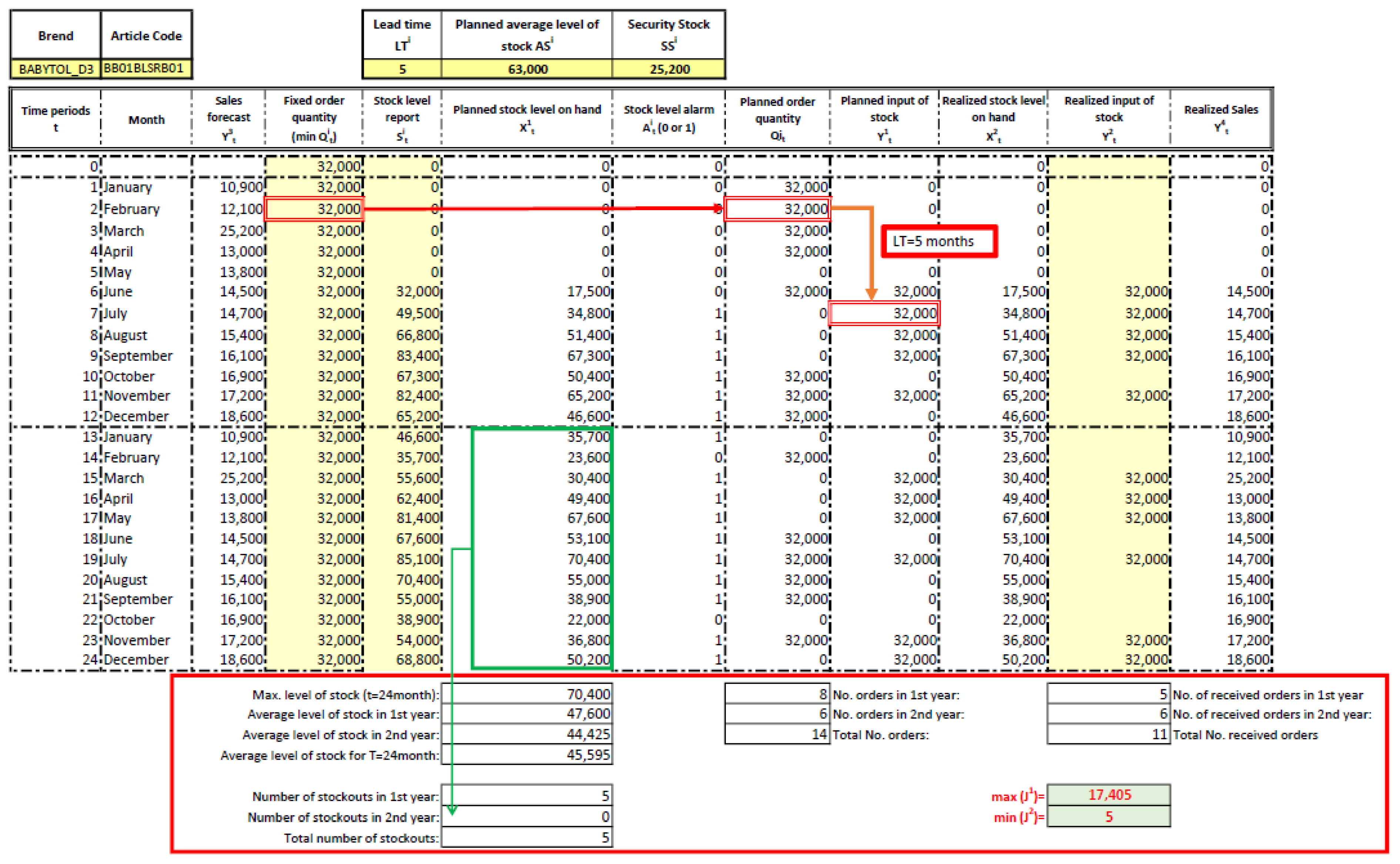
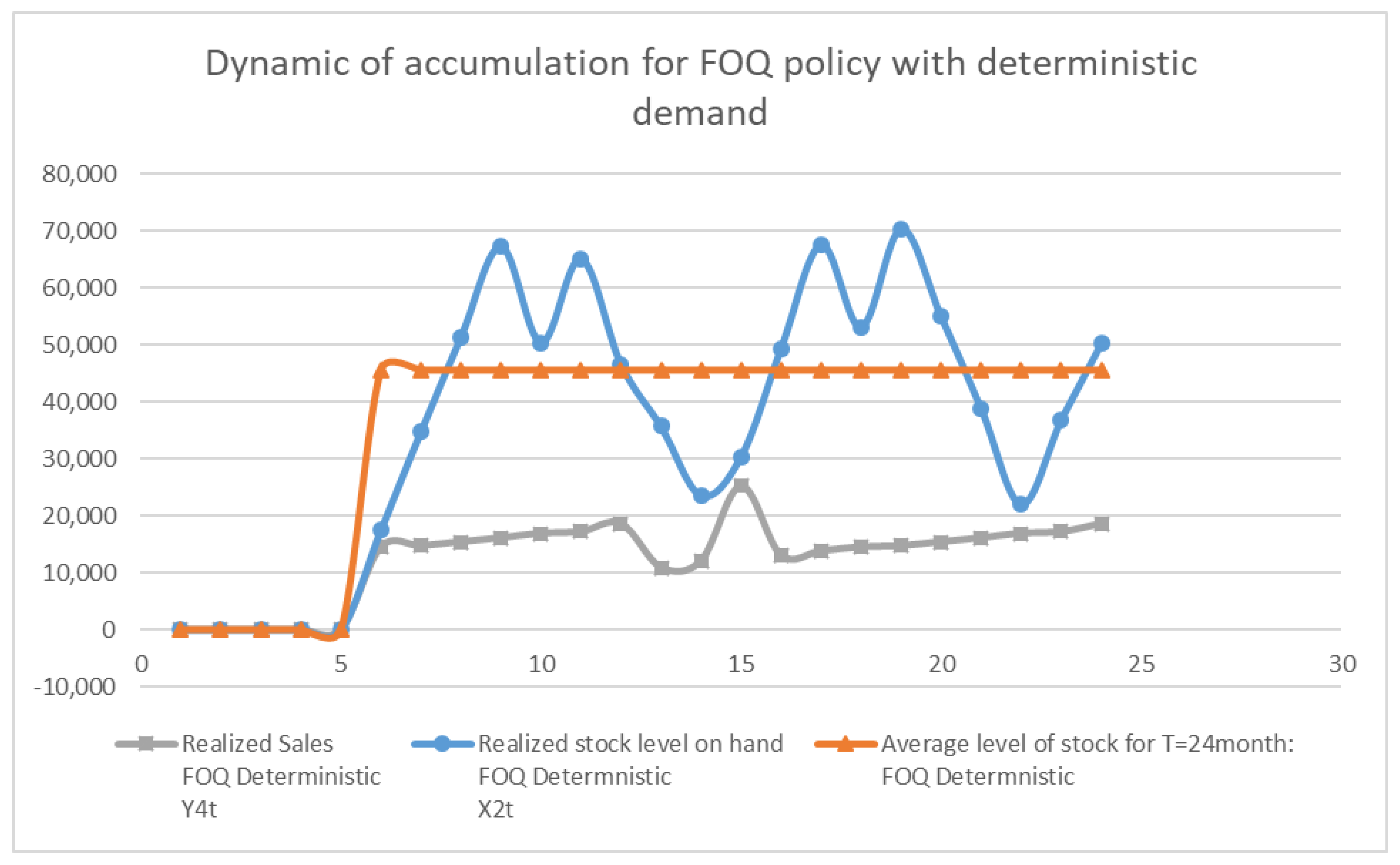
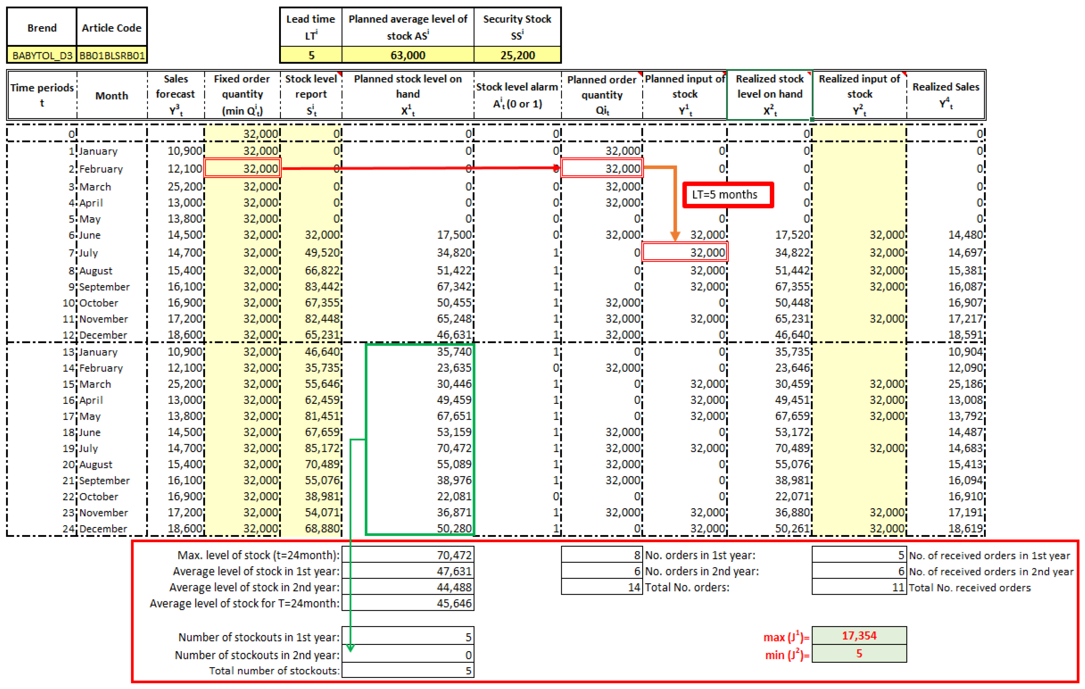
7.1. Instance 1: FOQ Ordering Policy

The following assumptions are considered for Instance 1:

• The initial level of inventory for products is zero in the case of launching a new product into the market. In this case, the first order will be launched at the beginning of January and delivered at the beginning of June (LT = 5 months).
• Based on historical data from previous years and experience, the manager forecasts monthly sales at the beginning of the first year for the next 2 years.
• The supplier defines the FOQ for each product. Since the FOQ is not unique for each product, the unit price depends on the ordered quantity.
• At the beginning of every month, customers from all countries send stock level reports to the company’s logistics manager. This report represents the prescribed form and format in an Excel spreadsheet.
• The delivery lead time is five months. The quantity ordered at the beginning of February is in stock at the beginning of July.
• At the beginning of the first year, there are no realized inputs of stock for launched orders from the previous periods.

Instance 1 is analysed for two separate cases. Case 1 considers FOQ policy with deterministic demand, where the forecasted sale is equal to the realized sale. Case 2 reflects FOQ policy with stochastic demand, when the realized sale is the forecasted sale changed randomly in range ±20%.

In Case 1, regulators $Y_t^3=Y_t^4=Sales forecast=known$, $t=\overline{1,24}$. From the beginning of June there are no stock-out situations, with exception of the first 5 months when the system waits for the delivery of the initial inventory (Figure 6).

In addition, except for the first five months, the value of the objective function defined by Equation (16) is 0, without stock-out situations (Figure 7).

According to Case 2 (Figure 8), the variable Realized sales is presented as the variable Sales forecast, which is changed randomly in the range of ±20% for each period of time horizon T, as it is presented by Equation (8).

For Case 2, the total number of planned orders and received deliveries is the same as for Case 1. From the company manager’s point of view, forecasted sales never deviate more than ±20%. This stochastic demand generates very similar values of the objective functions $J^1$ and $J^2$ as for Case 1, concerning the average level of inventories and stock-outs (Figure 9).

The numerical results of Case 1 and Case 2 for Instance 1 are presented in

Table 2. Numerical results of Case 1 and Case 2 for Instance 1.

No.	Instance 1: FOQ Ordering Policy	Case 1: Deterministic Demand	Case 2: Stochastic Demand
1	Lead time (month)	5	5
2	Planned average level of stock (unit)	63,000.00	63,000.00
3	Security stock (unit)	25,200.00	25,200.00
4	Max level of stock T = 24 months (unit)	70,400.00	70,472.00
5	Average level of stock T = 24 months (unit)	45,595.00	45,646.00
6	Total number of stock outs	5	5
7	Total number of launched orders	14	14
8	Total number of received orders	11	11
9	max (J1) = (2)–(5)	17,405.00	17,354.00
10	min (J2) = (6)	5	5

.

The total number of planned orders is 14, and the total number of received deliveries is 11. As shown in Figure 6 and Figure 8 and Table 2, at the beginning of the first year, the columns Stock level report, Realized input of stock and Realized sales are empty because there are no launched orders from the previous year for delivery in the first five months of time horizon T. For Case 1, the model shows that the planned average level of inventory for the product in the warehouse (63,000 units) is greater than the realized average level of stock in time horizon T = 24 months (45,595 units) for 17,405 units, according to the objective function (15). In addition, except for the first five months, the value of the objective function (16) is zero, without stock-out situations.

If we compare the numerical results of Case 1 and Case 2 for FOQ ordering policy (Table 2), it can be appointed that the differences between the values of the objective functions are small, even in Case 2, when the realized sales are randomly changed in the range of ±20%. An insignificant deviation of the objective functions results for Cases 1 and 2 confirms that the model is sensitive and stable. One of the main questions related to future research, also significant from a company perspective, can be: “What will happen with the Total number of orders, Stock-outs, and Costs, if the business environment is unstable and uncertainty is higher, e.g., if realized sales vary more than ±30% or ±50%?”.

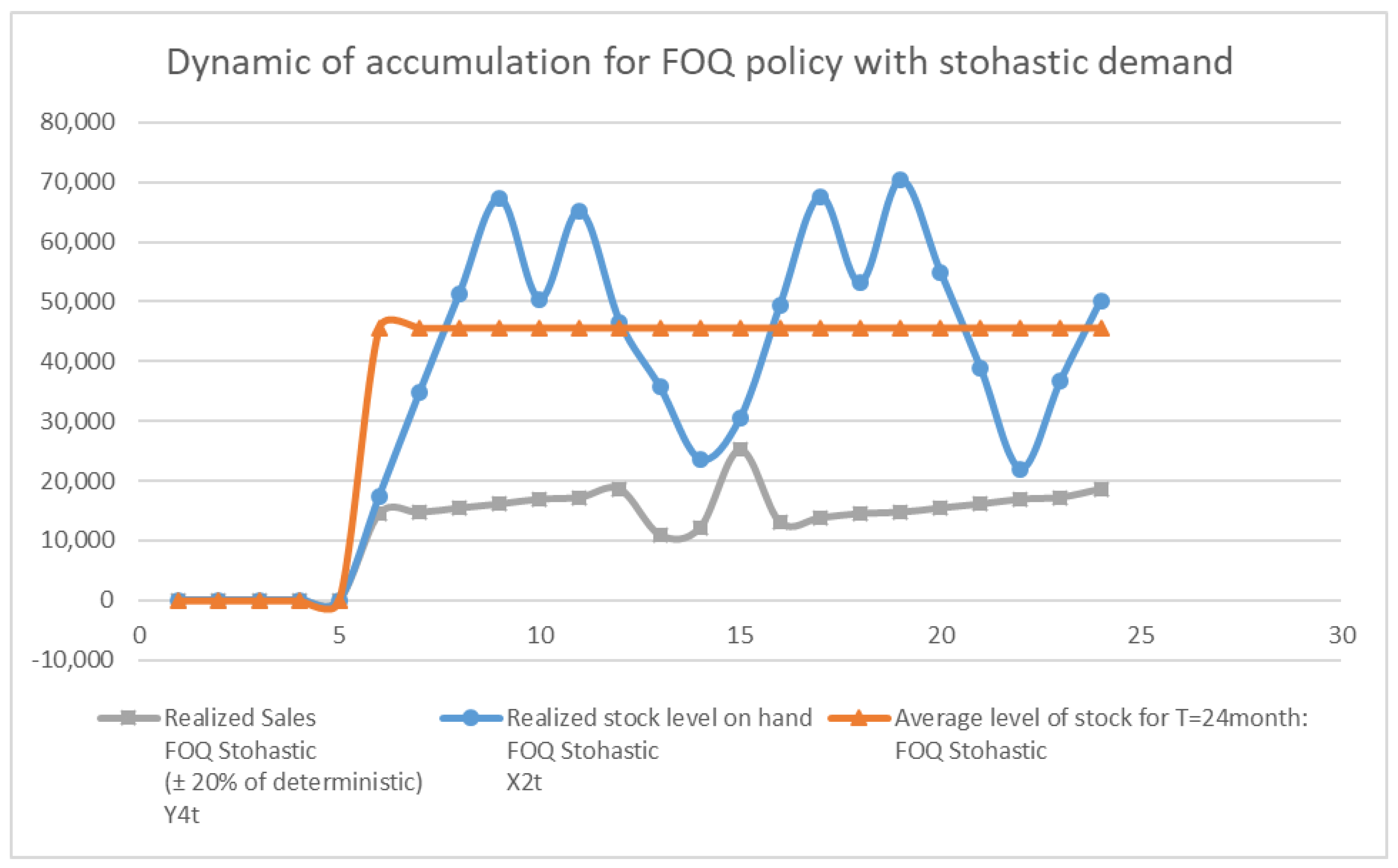
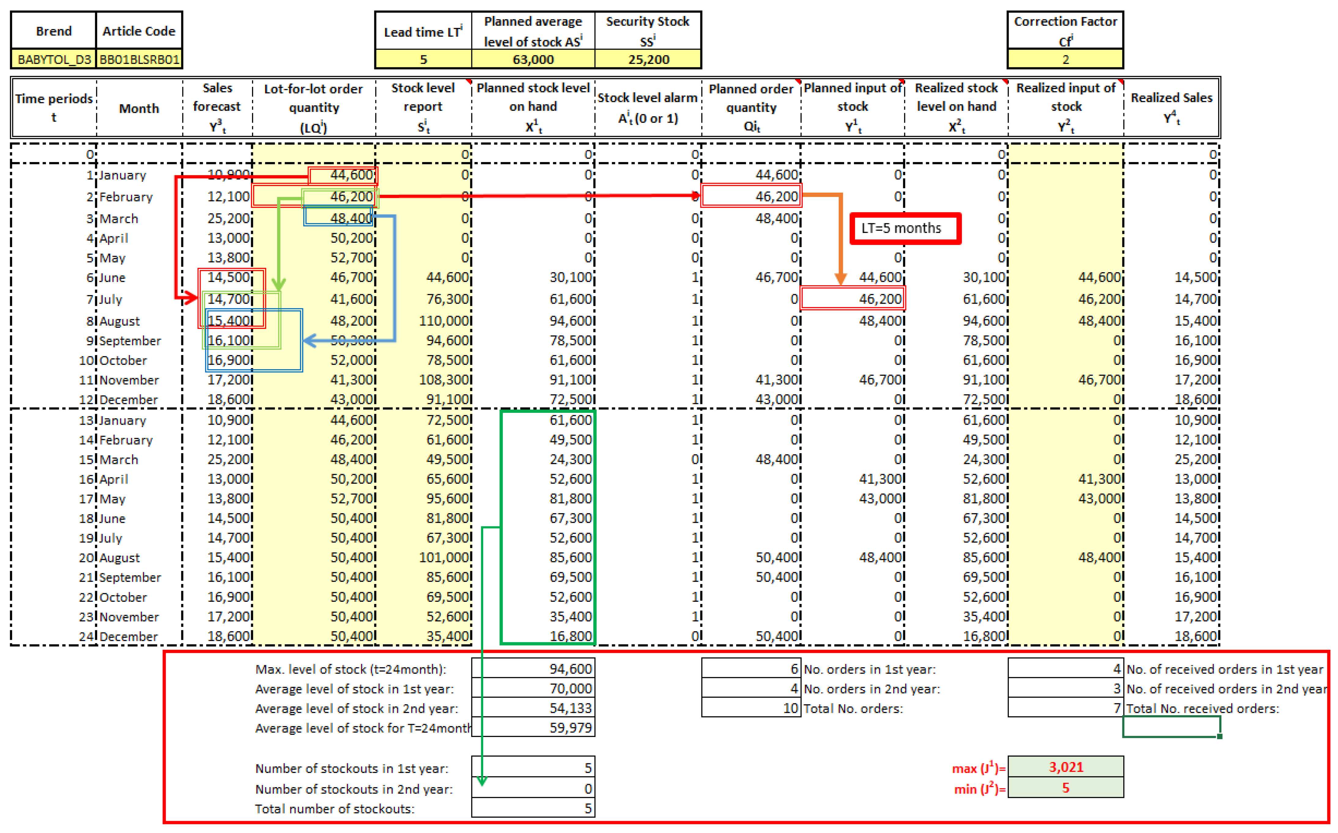
7.2. Instance 2: LFL Ordering Policy

In the case of LFL ordering policy, the order quantity is calculated in accordance with the moving horizon, i.e., the forecasted sales for three months which occurs after the expiry of the defined lead time. The variable $L{Q}_t^i$ (Equation (17)) represents the order quantity for the LFL model. General assumptions for Instance 2 are the same as for Instance 1. Instance 2 is analysed for two separate cases, as well as Instance 1. Case 1 considers LFL ordering policy with deterministic demand, where the forecasted sale is equal to the realized sale. Case 2 reflects LFL ordering policy with stochastic demand, where the realized sales are the forecasted sales changed randomly in the range ±20%. For Case 1, shown in Figure 10, regulators $Y_t^3=Y_t^4=Sales forecast=known$, $t=\overline{1,24}$.

As mentioned, Case 2 considers LFL ordering policy with stochastic demand. The variable realized sales is described by Equation (8). Except for the values of this variable, elements of the spreadsheet model for Case 2 are the same as for Case 1. Since the dynamic of accumulation for both cases of Instance 2 is pretty similar as for Instance 1, there was no need for graphic representation. For Case 2 of Instance 2, the total number of planned orders and received deliveries is the same as for Case 1 of Instance 2. The numerical results of Case 1 and Case 2, for Instance 2, are presented in

Table 3. Numerical results of Case 1 and Case 2 for Instance 2.

No.	Instance 2: LFL Ordering Policy	Case 1: Deterministic Demand	Case 2: Stochastic Demand
1	Lead time (month)	5	5
2	Planned average level of stock (unit)	63,000.00	63,000.00
3	Security stock (unit)	25,200.00	25,200.00
4	Max level of stock T = 24 months (unit)	94,600.00	94,599.00
5	Average level of stock T = 24 months (unit)	59,979.00	59,967.00
6	Total number of stock outs	5	5
7	Total number of launched orders	10	10
8	Total number of received orders	7	7
9	max (J1) = (2)–(5)	3021.00	3033.00
10	min (J2) = (6)	5	5

.

If we compare the numerical results of Case 1 and Case 2 for LFL ordering policy (Table 3), it can be noted that the differences between the values of the objective functions are small, even in Case 2, when the realized sales are randomly changed in the range of ±20%. An insignificant deviation of the objective functions results for Cases 1 and 2 confirms that the model is sensitive and stable.

7.3. Comparison of Numerical Results for Instance 1 and Instance 2

A comparative review of results for Instances 1 and 2 in the situation of deterministic demand is shown in

Table 4. Comparison of numerical results for Instance 1 and Instance 2 in Case 1.

No.	Parameters	Instance 1: FOQ Ordering Policy Case 1: Deterministic Demand	Instance 2: LFL Ordering Policy Case 1: Deterministic Demand	$\mathbf{\Delta }$ (Instance 1–Instance 2)
1	Lead time (month)	5	5	0
2	Planned average level of stock (unit)	63,000.00	63,000.00	0
3	Security stock (unit)	25,200.00	25,200.00	0
4	Max level of stock T = 24 months (unit)	70,400.00	94,600.00	24,200.00
5	Average level of stock T = 24 months (unit)	45,595.00	59,979.00	14,384.00
6	Total number of stock outs	5	5	0
7	Total number of launched orders	14	10	−4
8	Total number of received orders	11	7	−4
9	max (J1) = (2)–(5)	17,405.00	3021.00	−14,384.00
10	min (J2) = (6)	5	5	0

. The value of the objective function $J^1$ is decreased for 14,384 units, i.e., to the amount of 3021 units for the LFL ordering policy. The average level of inventories is increased by 14,384 units, which is a consequence of the decreased number of launched and received orders. The number of planned and realized deliveries is decreased by four, which significantly impacts delivery costs, but the average order quantity is also increased from 32,000 units (Figure 6) to 48,338 units (Figure 10). The decreased number of deliveries drives the increase of the average inventory level. Except for the first five months, the criterion function $J^2$ is zero, i.e., without stock-out situations.

However, if we compare the numerical results of Case 2 for Instance 1 and Case 2 for Instance 2 (

Table 5. Comparison of numerical results for Instance 1 and Instance 2 in Case 2.

No.	Parameters	Instance 1: FOQ Ordering Policy Case 2: Stochastic Demand	Instance 2: LFL Ordering Policy Case 2: Stochastic Demand	$\mathbf{\Delta }$ (Instance 1–Instance 2)
1	Lead time (month)	5	5	0
2	Planned average level of stock (unit)	63,000.00	63,000.00	0
3	Security stock (unit)	25,200.00	25,200.00	0
4	Max level of stock T = 24 months (unit)	70,472.00	94,599.00	24,127.00
5	Average level of stock T = 24 months (unit)	45,646.00	59,967.00	14,321.00
6	Total number of stock outs	5	5	0
7	Total number of launched orders	14	10	−4
8	Total number of received orders	11	7	−4
9	max (J1) = (2)–(5)	17,354.00	3033.00	−14,321.00
10	min (J2) = (6)	5	5	0

), the number of orders and consequently delivery costs are decreased. Therefore, based on previously declared assumptions of this control model, taking into account the defined objective functions (15) and (16), the performed numerical experiments show that the FOQ gives better results than the LFL policy.

The FOQ ordering policy will decrease the average amount of inventories and increase the stability in the supplier production process, i.e., the production series will be based on FOQ quantity. Nevertheless, considering the delivery costs, which are not assumptions of this model, the LFL policy could obtain better results than the FOQ policy due to the impact of the decreased number of deliveries.

Moreover, for the LFL ordering policy (Table 5), the total number of launched and received orders is decreased for four orders. Bearing in mind that the average lead time of delivery is five months, the waiting time for deliveries is decreased by 20 months, and the risk of undelivered orders is much lower.

8. Conclusions

This paper describes a multiproduct inventory control problem in a pharmaceutical distribution company, modelled as a corresponding dynamic discrete-time system control process. The actuality of the topic elaborated in the paper is consistent with the importance of the pharmaceutical inventory and distribution management. The improvement of the mentioned processes management in pharmaceutical companies implies cost reduction and customer service level improvements.

The paper is aimed at the development of an inventory control model for a pharmaceutical distribution company, with an emphasis on reorder quantities and reorder periods, and the satisfaction of specific constraints. The mathematical model is based on the proposed conceptual model, developed in accordance with the modern control theory concept and specific practical assumptions and constraints of the supply chain, as noticed in the company. The authors proposed two variations of the model, implemented in the spreadsheet environment of MS Excel and automated through Visual Basic for Applications. The model allows analysis from many different perspectives and can be easily modified and enhanced in order to reflect new scenarios. The developed model represents a baseline model that enables the creation of alternative scenarios and comparison of those scenarios to the baseline. Furthermore, the presented solution of the problem satisfies the request defined by the company which is related to the affordable but dynamic and flexible software solution that is relatively easy to implement and use. These contributions, detailed in the paper, represent an important aspect of managerial implications.

The theoretical contribution and some of the main advantages of the developed control model concerning the traditional DRP model are:

–

FOQ- and LFL-based models determine lot size and safety stock.

–

These models recalculate order quantities and reorder points if demand is changed in real-time.

–

The full automation of the model is based on the concept of feedback control.

–

The structure of the model is precisely defined according to the object of discrete control with an adequate mathematical apparatus.

In order to emphasize specificities of the research presented in this paper, and at the same time the improvements of the previous study mentioned in [15], the authors of the paper point out the following contributions:

–

Modern control theory (MCT), i.e., self–regulation and feedback control concepts, with relevant elements (sensor, comparator, controller, system) of the feedback loop are applied during the development of the conceptual model.

–

The mathematical model presented in the paper is comprised of two flows. The planned inventory state represents information flow, while the actual inventory state refers to material flow. Each flow has one phase of accumulation and two phases of action. Two sales variables and two inventory state variables, planned and realized, are precisely mathematically defined, with their mutual influence, i.e., the impact of the actual state of inventory on the future, and the planned inventory state.

–

The performance criterion of the inventory system is defined and described through two objective functions, the maximization of the difference between the planned average inventory level and the realized average inventory level and the minimization of the number of stock-out situations.

–

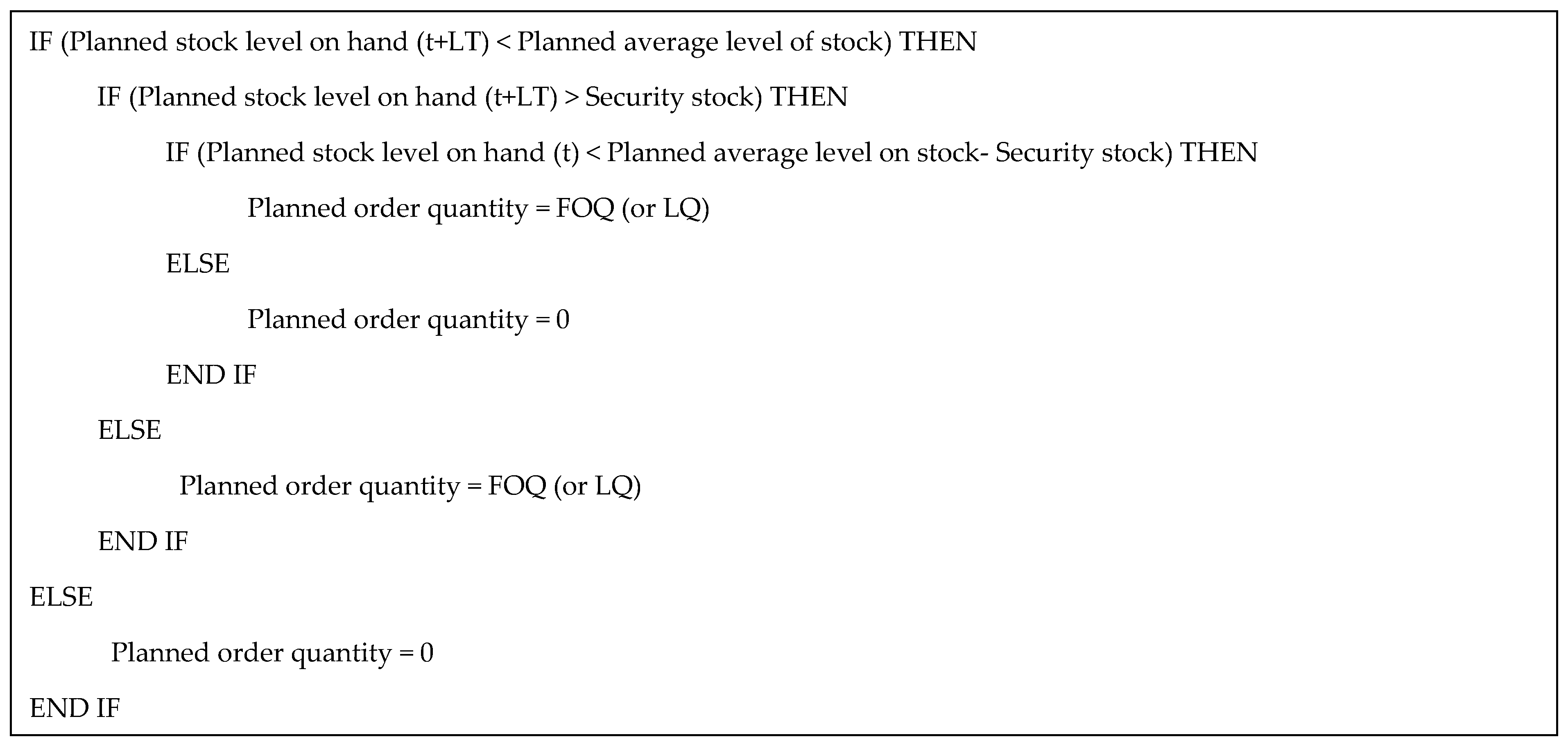
The originally developed comparison algorithm for the planned order quantity reflects the decision tree for comparison of all relevant stock variables.

–

Sensitivity analysis is conducted, and numerical results are explained clearly with all supporting data.

–

Stochastic demand is generated as a random variation of sales forecast in the range of ±20%. Numerical results are compared for deterministic and stochastic actual sales.

The applicability of the model has been proven by its usage for procurement planning in the described company within the period of two years. The created plan comprised more than 50 products per country for several countries from Eastern-Central Europe. Research directions imply further research of the model efficiency for real-life problems but with larger dimensions. For example, the number of units and constraints could be increased, the model could include delivery costs, and the stochastic demand could be randomly varied in a range more than ±20.

References

1. Hoque, M.E.; Paul, N. Inventory Management of Pharmaceutical Industries in Bangladesh. In Proceedings of the International Conference on Mechanical Engineering 2011 (ICME2011), Dhaka, Bangladesh, 18–20 December 2011. [Google Scholar]
2. Uthayakumar, R.; Priyan, S. Pharmaceutical supply chain and inventory management strategies: Optimization for a pharmaceutical company and a hospital. Oper. Res. Health Care 2013, 2, 52–64. [Google Scholar] [CrossRef]
3. Management Sciences for Health. MDS-3: Managing Access to Medicines and Health Technologies; Management Sciences for Health: Arlington, VA, USA, 2012. [Google Scholar]
4. Axsäter, S. Inventory Control; Springer: Berlin/Heidelberg, Germany, 2015; Volume 225. [Google Scholar] [CrossRef]
5. Kwak, C.; Choi, J.S.; Kim, C.O.; Kwon, I.H. Situation reactive approach to vendor managed inventory problem. Expert Syst. Appl. 2009, 36, 9039–9045. [Google Scholar]
6. Grob, C. Inventory Management in Multi-Echelon Networks: On the Optimization of Reorder Points; Springer: Berlin/Heidelberg, Germany, 2018; Volume 128. [Google Scholar]
7. Qiu, Y.; Qiao, J.; Pardalos, P.M. Optimal production, replenishment, delivery, routing and inventory management policies for products with perishable inventory. Omega 2019, 82, 193–204. [Google Scholar] [CrossRef]
8. Perez, H.D.; Hubbs, C.D.; Li, C.; Grossmann, I.E. Algorithmic Approaches to Inventory Management Optimization. Processes 2021, 9, 102. [Google Scholar]
9. Srinivasarao, G. Overview of Inventory Optimization in Operations Management. In Business Research and Innovation, Proceedings of the International Conference on Business Research and Innovation ICBRI 2021, Murshidabad, India, 26–27 February 2021; Excel India Publishers: New Delhi, India, 2021; pp. 486–492. [Google Scholar]
10. Settanni, E.; Harrington, T.S.; Srai, J.S. Pharmaceutical supply chain models: A synthesis from a systems view of operations research. Oper. Res. Perspect. 2017, 4, 74–95. [Google Scholar] [CrossRef] [Green Version]
11. Lemmens, S.; Decouttere, C.; Vandaele, N.; Bernuzzi, M. A review of integrated supply chain network design models: Key issues for vaccine supply chains. Chem. Eng. Res. Des. 2016, 109, 366–384. [Google Scholar] [CrossRef]
12. Fahimnia, B.; Farahani, R.Z.; Marian, R.; Luong, L. A review and critique on integrated production—Distribution planning models and techniques. J. Manuf. Syst. 2013, 32, 1–19. [Google Scholar] [CrossRef]
13. Nagurney, A.; Li, D. A supply chain network game theory model with product differentiation, outsourcing of production and distribution, and quality and price competition. Ann. Oper. Res. 2015, 226, 479–503. [Google Scholar] [CrossRef]
14. Agrell, P.J.; Hatami-Marbini, A. Frontier-based performance analysis models for supply chain management: State of the art and research directions. Comput. Ind. Eng. 2013, 66, 567–583. [Google Scholar]
15. Antic, S.; Djordjevic, L.; Lisec, A. Case study: Dynamic discrete model of fixed order point quantity system for inventories in pharmaceutical distribution. In Proceedings of the 21st International Symposium on Logistics (ISL 2016), Kaohsiung, Taiwan, 3–6 July 2016; pp. 455–462. [Google Scholar]
16. 4U Pharma. 4youpharma. 2018. Available online: http://4youpharma.com/ (accessed on 12 April 2019).
17. Vila-Parrish, A.R.; Ivy, J.S. Managing supply critical to patient care: An introduction to hospital inventory management for pharmaceuticals. In Handbook of Healthcare Operations Management; Springer: New York, NY, USA, 2013; pp. 447–463. [Google Scholar]
18. Li, J.; Liu, L.; Hu, H.; Zhao, Q.; Guo, L. An inventory model for deteriorating drugs with stochastic lead time. Int. J. Environ. Res. Public Health 2018, 15, 2772. [Google Scholar] [CrossRef] [Green Version]
19. Khodaverdi, R.; Shahbazi, M.; Azar, A.; Fathi, M.R. A Robust Optimization Approach for Sustainable humanitarian supply chain management of blood products. Int. J. Hosp. Res. 2022, 11. Available online: http://ijhr.iums.ac.ir/article_139129.html (accessed on 20 January 2022).
20. Zandieh, M.; Janatyan, N.; Alem-Tabriz, A.; Rabieh, M. Designing sustainable distribution network in pharmaceutical supply chain: A case study. Int. J. Supply Oper. Manag. 2018, 5, 122–133. [Google Scholar]
21. Narayana, S.A.; Arun, E.A.; Rupesh, P.K. Reverse logistics in the pharmaceuticals industry: A systemic analysis. Int. J. Logist. Manag. 2014, 25, 379–398. [Google Scholar] [CrossRef]
22. Hansen, K.R.N.; Grunow, M. Planning operations before market launch for balancing time-to-market and risks in pharmaceutical supply chains. Int. J. Prod. Econ. 2015, 161, 129–139. [Google Scholar] [CrossRef]
23. Ahmadi, E.; Masel, D.T.; Metcalf, A.Y.; Schuller, K. Inventory management of surgical supplies and sterile instruments in hospitals: A literature review. Health Syst. 2019, 8, 134–151. [Google Scholar] [CrossRef] [PubMed]
24. Schmitt, A.J.; Sun, S.A.; Snyder, L.V.; Shen, Z.J.M. Centralization versus decentralization: Risk pooling, risk diversification, and supply chain disruptions. Omega 2015, 52, 201–212. [Google Scholar] [CrossRef]
25. Enns, S.T.; Suwanruji, P. Distribution planning and control: An experimental comparison of DRP and order point replenishment strategies. In Proceedings of the Academy of Business and Administrative Sciences, 2000 International Conference, Prague, Czech Republic, 10 July 2000. [Google Scholar]
26. Seok, H.; Nof, S.Y. Intelligent information sharing among manufacturers in supply networks: Supplier selection case. J. Intell. Manuf. 2018, 29, 1097–1113. [Google Scholar] [CrossRef]
27. Chapman, S.N.; Arnold, J.T.; Gatewood, A.K.; Clive, L.M. Introduction to Materials Management; Pearson Education Limited: New York, NY, USA, 2017. [Google Scholar]
28. Russell, R.S.; Taylor, B.W. Operation Management: Quality and Competitiveness in a Global Environment; John Wiley & Sons: New York, NY, USA, 2006; pp. 529–552. [Google Scholar]
29. Chase, R.; Aquilano, N. Operations Management for Competitive Advantage; IRWIN: New York, NY, USA, 2004; pp. 542–560. [Google Scholar]
30. Barlow, J.F. Excel Models for Business and Operations Management; John Wiley & Sons: New York, NY, USA, 2005; pp. 244–258. [Google Scholar]
31. Muller, M. Essentials of Inventory Management; Harper Collins Leadership: New York, NY, USA, 2019. [Google Scholar]
32. Wild, T. Best Practice in Inventory Management; Elsevier Science: London, UK, 2017; pp. 112–148. [Google Scholar]
33. Grubbström, R.W.; Bogataj, L.; Bonney, M.C.; Disney, S.C.; Tang, O. Inter-Linking MRP Theory and Production and Inventory Control Models. In Proceedings of the 13th International Working Conference on Production Economics, Igls, Austria, 16–20 February 2004. [Google Scholar]
34. Franco, C.; Alfonso-Lizarazo, E. A structured review of quantitative models of the pharmaceutical supply chain. Complexity 2017, 2017, 5297406. [Google Scholar] [CrossRef] [Green Version]
35. Saha, E.; Ray, P.K. Modelling and analysis of inventory management systems in healthcare: A review and reflections. Comput. Ind. Eng. 2019, 137, 106051. [Google Scholar] [CrossRef]
36. Bubnicki, Z. Modern Control Theory; Springer: Berlin/Heidelberg, Germany, 2002. [Google Scholar]
37. Antic, S.; Kostic, K.; Dordevic, L. Spreadsheet Model of Inventory Control Based on Modern Control Theory. In Proceedings of the 13th International Symposium SymOrg: Innovative Management and Business Performance, Zlatibor, Serbia, 5–9 June 2012. [Google Scholar]
38. Doyle, J.; Francis, B.; Tannenbaum, A. Feedback Control Theory; Macmillan Publishing Co.: Basingstoke, UK, 1990. [Google Scholar]
39. Zook, D.; Bonne, U.; Samad, T. Control Systems, Robotics and Automation; Eoloss publishers: Oxford, UK, 2009. [Google Scholar]
40. Andrei, N. Modern Control Theory-A historical perspective. Stud. Inform. Control 2006, 15, 51. [Google Scholar]
41. Aström, K.J.; Murray, R.M. Feedback Systems: An Introduction for Scientists and Engineers; Princeton University Press: Princeton, NJ, USA, 2010. [Google Scholar]
42. Azarskov, V.N.; Skurikhin, V.I.; Zhiteckii, L.S.; Lypoi, R.O. Modern Control Theory Applied to Inventory Control for a Manufacturing System. IFAC Proc. Vol. 2013, 46, 1200–1205. [Google Scholar] [CrossRef]
43. Ying, Z.; Weiguo, W.; Qiushuang, H.; Ye, X.; Hong, J. Inventory control based on a real-moment dynamic model. In Proceedings of the 2011 International Conference on Management Science and Industrial Engineering (IEEE), Harbin, China, 6–11 January 2011; pp. 838–841. [Google Scholar]
44. Shin, J.; Lee, J.; Park, S.; Koo, K.K.; Lee, M. Analytical design of a proportional-integral controller for constrained optimal regulatory control of inventory loop. Control Eng. Pract. 2008, 16, 1391–1397. [Google Scholar] [CrossRef]
45. Tako, A.A.; Robinson, S. The application of discrete event simulation and system dynamics in the logistics and supply chain context. Decis. Support Syst. 2012, 52, 802–815. [Google Scholar] [CrossRef] [Green Version]
46. Ossimitz, G.; Mrotzek, M. The Basics of System Dynamics: Discrete vs. Continuous Modelling of Time. In Proceedings of the 26th International Conference of the System Dynamics Society, Athens, Greece, 20–24 July 2008. [Google Scholar]
47. Kostić, K. Inventory control as a discrete system control for the fixed-order quantity system. Appl. Math. Model. 2009, 33, 4201–4214. [Google Scholar] [CrossRef]
48. Wagner, H.M.; Whitin, T.M. Dynamic version of the economic lot size model. Manag. Sci. 1958, 5, 89–96. [Google Scholar] [CrossRef]
49. Scarf, H. The Optimality of (s; S) Policies in the Dynamic Inventory Problem. In Mathematical Methods in the Social Sciences; Arrow, K.J., Karlin, S., Suppes, P., Eds.; Stanford University Press: Stanford, CA, USA, 1959. [Google Scholar]
50. Bertsekas, D.P. Dynamic Programming, Deterministic and Stochastic Models; Prentice-Hall: Englewood Cliffs, NJ, USA, 1987. [Google Scholar]
51. Jans, R.; Degraeve, Z. Meta-heuristics for dynamic lot sizing: A review and comparison of solution approaches. Eur. J. Oper. Res. 2007, 177, 1855–1875. [Google Scholar] [CrossRef]
52. Đorđević, L.; Antić, S.; Čangalović, M.; Lisec, A. A metaheuristic approach to solving a multiproduct EOQ-based inventory problem with storage space constraints. Optim. Lett. 2017, 11, 1137–1154. [Google Scholar] [CrossRef]
53. Antic, S.; Djordjevic, L.; Kostic, K.; Lisec, A. Dynamic discrete simulation model of an inventory control with or without allowed shortage. UPB Sci. Bull. Ser. A 2015, 77, 163–176. [Google Scholar]
Figure 1. Concept of the feedback loop, reproduced with permission from InstrumentationTools.com, 2021 [38].
Applsci 12 01536 g001
Figure 2. Elements of the feedback loop for the inventory control model.
Applsci 12 01536 g002
Figure 3. Graphical representation of information and material flows.
Applsci 12 01536 g003
Figure 4. Elements of the spreadsheet model.
Applsci 12 01536 g004
Figure 5. Pseudocode for planned order quantity.
Applsci 12 01536 g005
Figure 6. Elements of the spreadsheet model for Case 1: FOQ policy with deterministic demand.
Applsci 12 01536 g006
Figure 7. Dynamic of accumulation for Case 1: FOQ policy with deterministic demand.
Applsci 12 01536 g007
Figure 8. Elements of the spreadsheet model for Case 2: FOQ policy with stochastic demand.
Applsci 12 01536 g008
Figure 9. Dynamic of accumulation for Case 2: FOQ policy with stochastic demand.
Applsci 12 01536 g009
Figure 10. Elements of the spreadsheet model for Case 1: LFL policy with deterministic demand.
Applsci 12 01536 g010