Different Types of Continuous Track Irregularities as Sources of Train-Induced Ground Vibration and the Importance of the Random Variation of the Track Support

Abstract

Irregularities of the track are a main cause of train-induced ground vibration, and track maintenance is of great importance. Although geometric irregularities at the wheel-rail contact are widely used, other types of irregularities, such as stiffness irregularities, irregularities from different track positions and irregularities in the wave propagation, were analysed in the present study. The track behaviour was investigated by a multi-beam-on-soil model. This track model is coupled with a vehicle model to calculate the vehicle–track interaction. The track model was also used for the track filtering, which transfers a track support error to the equivalent rail irregularity or, conversely, the sharp axle pulse on the rail to a smoother pulse on the soil. In the case in which this filtering varies randomly along the track, the pulses of the moving static load induce a certain ground vibration component (“the scatter of axle pulses”). This effect was calculated by the superposition of axle pulses in the frequency domain and by a stochastic simulation. Simultaneous vehicle, track and soil measurements at a certain site were used to evaluate the different excitation and ground vibration components. The agreement between calculations and axle-box and soil measurements is good. The ground vibrations calculated from rail irregularities and corresponding dynamic loads, however, clearly underestimate the measured ground vibration amplitudes. Only the static load that is moving over a varying track support stiffness can produce the important mid-frequency ground vibration component by the scatter of axle pulses.

1. Introduction

Irregularities are the main source if excitation of train-induced ground vibrations, which are in the frequency range of 4 to 100 Hz (maximal 250 Hz). Irregularities can be divided into vertical, horizontal, rotational and gauge errors; vehicle and track irregularities; and low-frequency alignment errors and high-frequency roughness errors, where the areas of interest of the present article are underlined. The irregularities are presented as wavelength or wavenumber spectra. Some normative alignment spectra from US, China, France, and Germany are presented and compared in [1]. Measurement examples of track errors are given, for example, in [2,3]. The track errors in the present article are based on own axle-box measurements at a ground vibration measurement site [4]. The article is focused on the mid-frequency range of 8 to 30 Hz, which is usually the dominant ground vibration in the mid and far field.

In ground vibration analysis, different numerical models of the railway track and the soil have been established: the wavenumber-domain models [5,6,7,8], finite/infinite-element models [9,10,11,12] (SBFEM), boundary-element models [13,14], and 2.5D coupled wavenumber-domain (finite or boundary-element) models [5,15,16,17]. The present contribution is based on frequency-wavenumber methods and their approximations; see Appendix A. The additional method of superposition of axle pulses was also used in [18] for trans-Rayleigh trains that are moving faster than the waves in the soil; however, these are not included in the present contribution.

When the theoretical models are compared with measurements, the geometric irregularities at the wheel–rail contact are used as the excitation in most cases. Moreover, the irregularities from the US standard [2], which are quite high, are often used. For some model verifications, the irregularities are measured [5,8,17,19] mainly by hand-driven trolleys, which are suitable for roughness and for which the results must be extrapolated to low frequencies. In [19], a low-frequency method was used in addition to the high-frequency roughness measurement and the combined results showed an almost unique curve. Axle-box measurements [4,5] provide results for a wide frequency range and include track and vehicle irregularities that can be distinguished by their different frequency characteristics [20]. In all these cases, the inertial forces of the wheelset running over the irregularities are understood as the excitation of the ground vibration.

In addition to track and vehicle irregularities, the following irregularities can be distinguished: rail unevenness or roughness [21] and wheel unevenness or roughness, which are both at high frequencies above 50 Hz and are not covered in this article; low order wheel out-of-roundness between 10 and 50 Hz [22]; geometric track alignment or level errors, geometric track support errors and track support stiffness variations usually below 30 Hz [23,24,25]; and deterministic track stiffness variation with sleeper-distance frequency above 50 Hz [26]. All these irregularities generate dynamic axle loads when an axle (the unsprung mass) passes over these irregularities [27]. An additional effect follows from the passage of a static load over a track with an irregular track support (irregular ballast, irregular soil, irregular sleeper contact). The randomly varying track support stiffness was analysed experimentally in [28,29,30], and it is known that the track support can strongly vary up to hanging sleepers. In the case of varying track stiffness, the ground vibration is generated in a different way by the irregular transfer of the static load to the ground.

The structure of this article is as follows. First (Section 2), the importance of the mid-frequency ground vibration component is illustrated by measurements at two sites. In Section 3, all theoretical methods are described, namely, the track analysis by a multi-beam-on-soil model, the vehicle–track interaction for the force transfer functions, the track filtering for geometric track support errors, a two-step linear perturbation analysis for the support stiffness variation, and the regular and irregular superposition of the axle pulses on all sleepers by a stochastic simulation. In Section 4, the calculated force transfers and ground vibrations for all excitations are presented. Finally, the detailed results (acceleration, irregularity, and force spectra, and ground vibration amplitudes and spectra) of a measurement site are compared with the calculations in Section 5.

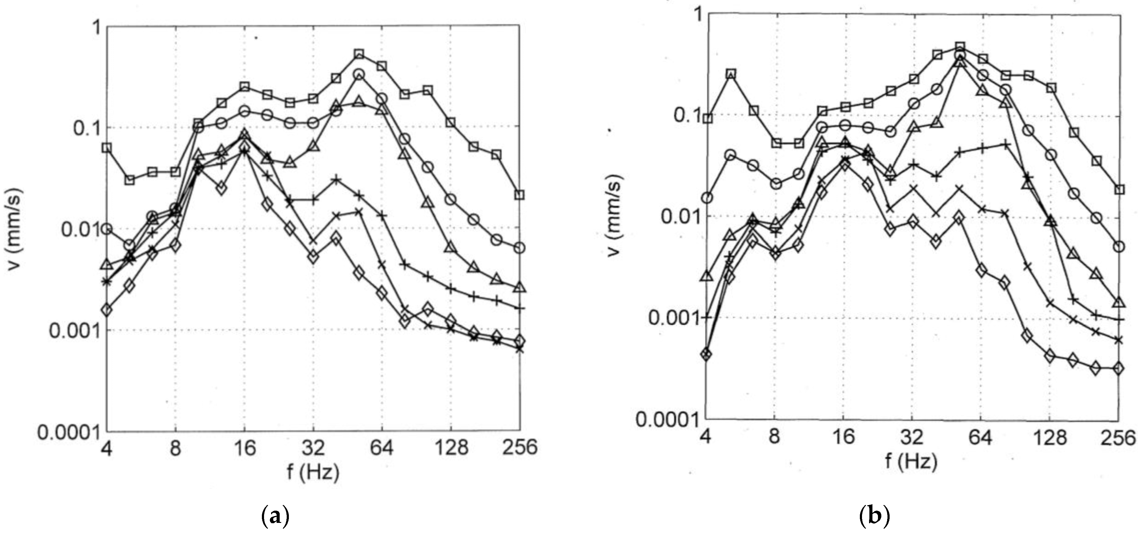
2. Experimental Motivation by the Dominant Frequency Range of Railway-Induced Ground Vibration

This article was motivated by experimental observations of railway-induced ground vibration. The ground vibration was measured by geophones (velocity transducers), filtered and amplified, digitised with a frequency of 2 kHz in a 72-channel measurement system. An instrumented impact hammer was used for artificial excitation and yields the force signal to evaluate transfer functions (Section 5.2).

Two examples are shown in Figure 1—the passage of standard passenger trains at site N with soft clayey soil (shear wave velocity v_S = 150 m/s), train speed v_T ≈ 100 km/h, and at site H with sandy, medium stiff soil (v_S = 225 m/s) and a train speed of v_T ≈ 160 km/h. A third site W is analysed in Section 5.3, where a special passenger train was run with specific train speeds between 63 and 160 km/h, at least three times for each speed. The standard trains were measured 10 to 15 times with slightly varying speed.

The train induced ground vibrations of site N and site H are shown in Figure 1 for the distances between 3 and 50 m as one-third octave band spectra of the whole frequency range from 4 to 256 Hz. The response can be roughly divided into three frequency ranges. The low frequencies have only small amplitudes (except sometimes the first measurement point). The high frequencies have a strong attenuation with distance so that the further distances have small amplitudes. The mid-frequency range from 8 to 30 Hz has a weak attenuation and has therefore the greatest amplitudes in some distance. Therefore, the mid frequencies are the most important frequency range in most situations, and the analysis of the present contribution is focused on this important mid-frequency range.

3. Frequency Domain Methods of Calculation

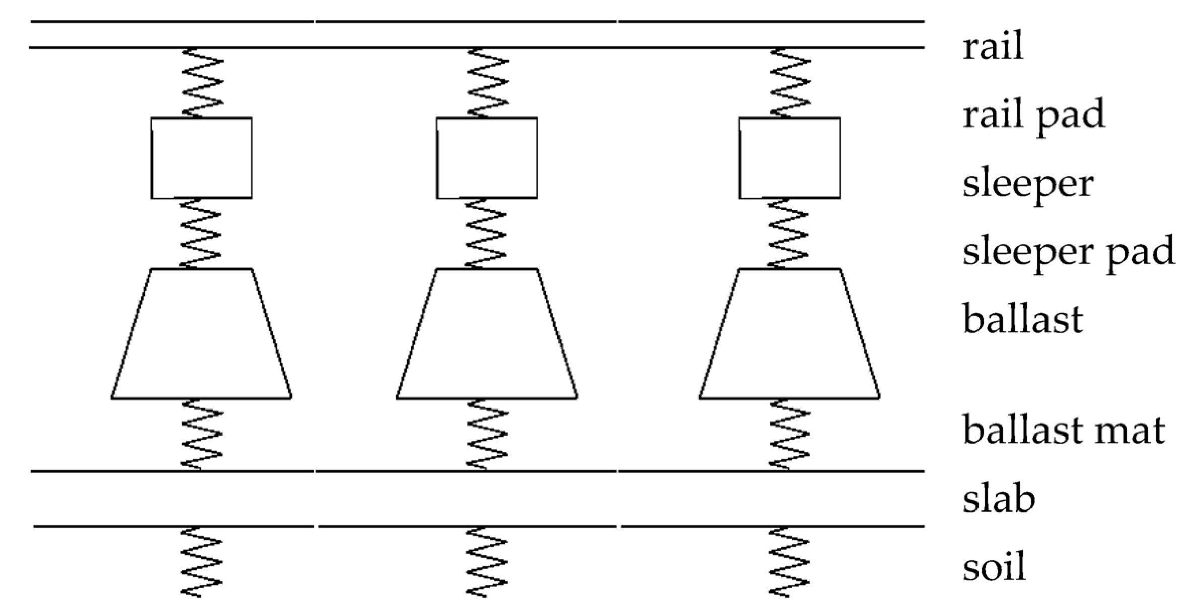
3.1. Simple Vehicle and Multi-Beam-on-Soil Track

The dynamic stiffness K_V of the vehicle can be approximated by the mass m_W of the wheelset and the circular frequency ω as:

$$K_V\left(\omega \right)=-m_W{\omega }^2$$

(1)

The minor effects of more detailed vehicle models have been discussed in [31].

Many track systems have been calculated by the combined finite-element boundary-element method [32] or by a faster multi-beam-on-soil track model in the frequency-wavenumber domain (Figure 2) as follows. The track model consists of n beams that represent the rails and track slabs, and which are described by the bending stiffnesses EI_j and the masses per length m_j’ in the diagonal matrices EI and M, and by a stiffness and damping matrix K and C representing rail pads, sleepers, the ballast and any isolation element. The multi-beam system fulfils the set of differential equations for the displacements u and the load (per length) F′_T:

$$EI\frac{{\partial }^{4}u}{\partial y^4}+M\frac{{\partial }^{2}u}{\partial t^2}+C\frac{\partial u}{\partial t}+Ku={F^{\prime }}_{\mathrm{T}}$$

(2)

This equation is transformed to the frequency-wavenumber domain with wavenumber ξ:

$$({\xi }^{4}EI-{\omega }^{2}M+\mathrm{i}\omega C+K)u\left(\omega ,\xi \right)=({\xi }^{4}EI+K_{\mathrm{TS}}\left(\omega ,\xi \right))u\left(\omega ,\xi \right)={F^{\prime }}_{\mathrm{T}}\left(\omega ,\xi \right)$$

(3)

where K_TS(ω,ξ) = K_T(ω) + K_S(ω,ξ) is the dynamic track–soil stiffness matrix. The track stiffness K_T(ω) is calculated by transfer matrices for each support element [33], and the soil stiffness K_S(ω,ξ) = k_S(ω,ξ)e_n^Te_n is added to the last diagonal element. The soil stiffness k_S(ω,ξ) is calculated as a wavenumber integral and can be approximated by a Winkler approach k_S*(ω) = k_W + iωc_W (see Appendix A).

The dynamic track stiffness K_T(ω) between the axle load F_T and the corresponding rail displacement u_R can be calculated from the wavenumber integral:

$$\frac{1}{K_T\left(\omega \right)}=\frac{u_{\mathrm{R}}}{F_T}\left(\omega \right)=\frac{1}{2\mathsf{\pi }}{\int }_{-\infty }^{\infty }{e}_1{}^{\mathrm{T}}{\left(EI{\xi }^4+K_{\mathrm{TS}}\left(\omega ,\xi \right)\right)}^{-1}{e}_1\mathrm{d}\xi$$

(4)

The force F_S on the soil follows from the displacement u_S of the soil and the soil stiffness k_S as:

$$F_{\mathrm{S}}\left(\omega \right)=k_{\mathrm{S}}{u}_{\mathrm{S}}\left(\omega ,\xi =0\right)=k_{\mathrm{S}}\left(\omega ,\xi =0\right)e_n{}^{\mathrm{T}}{K}_{\mathrm{TS}}{\left(\omega ,\xi =0\right)}^{-1}{e}_1{F}_{\mathrm{T}}=H_{\mathrm{T}}\left(\omega \right)F_{\mathrm{T}}\left(\omega \right)$$

(5)

The base vector e₁ stands for the top of the track, the base vector e_n stands for the bottom of the track (the soil).

3.2. The Vehicle-Track Transfer Functions

The dynamic stiffness K_T(ω) of the track is coupled with the dynamic stiffness K_V(ω) of the vehicle to analyse the combined vehicle–track system. The force F_T that acts on the track is calculated as:

$$F_{\mathrm{T}}\left(\omega \right)=-\frac{K_{\mathrm{V}}\left(\omega \right)K_{\mathrm{T}}\left(\omega \right)}{K_{\mathrm{V}}\left(\omega \right)+K_{\mathrm{T}}\left(\omega \right)}s\left(\omega \right)=H_{\mathrm{V}}\left(\omega \right) s\left(\omega \right)$$

(6)

for the geometric vehicle–track irregularities s(ω). In the case of a varying track stiffness K_T(x) (see Section 3.4), a similar transfer function H_V*(ω) for the effective track irregularities s*(ω) yields:

$$F_{\mathrm{T}}\left(\omega \right)=-\frac{K_{\mathrm{V}}\left(\omega \right)K_{\mathrm{T}0}}{K_{\mathrm{V}}\left(\omega \right)+K_{\mathrm{T}}\left(\omega \right)}{s}^{*}\left(\omega \right)=H_V{}^{*}\left(\omega \right) s^{*}\left(\omega \right)$$

(7)

The only difference is that the static track stiffness K_T0 is used in the numerator [34]. Equation (7) holds also for the effective irregularity s_D* due to the stiffness variation on and between the sleepers.

In general, the influence of the track mass must be introduced by the force transfer function H_T(ω) = F_S/F_T(ω) in Equation (5) from the top to the bottom of the track. Finally, the force F_S on the soil, which excites the ground vibration, can be calculated as:

$$F_S\left(\omega \right)=H_{\mathrm{T}}\left(\omega \right)F_{\mathrm{T}}\left(\omega \right)=H_{\mathrm{T}}\left(\omega \right)H_{\mathrm{V}}\left(\omega \right)s\left(\omega \right).$$

(8)

For the standard ballast track and the interesting frequency range (8–30 Hz), the track transfer H_T(ω) is almost 1, so that the force on the track is nearly the force on the soil F_T ≈ F_S = F (the dynamic axle load).

3.3. Irregularities at the Vehicle-Track Interface

The mostly referenced causes of train-induced ground vibrations are geometric irregularities of the vehicle and the track, which are most simply described as geometric irregularities s at the interface between wheel and rail. Irregularities can also come from other positions in the track [23], and, most importantly, from the track support. Moreover, irregularities are not only geometric irregularities, but can also be due to a stiffness variation. All irregularities can be transformed to effective irregularities at rail level s*, s_R and the dynamic loads follow with the vehicle–track transfer function (6), (7). The effects of the geometric or stiffness variation of the track support are presented in the next section.

3.4. Irregularities of the Track Support and Track Filtering

3.4.1. Geometric Irregularities of the Track Support

At first, the track is excited by a harmonic irregularity of the soil surface:

$${\mathit{s}}_{\mathit{S}}\left(\xi \right)=s_S{e}^{i\xi x}{\mathit{e}}_{\mathit{n}}.$$

(9)

The response u to this excitation is also a harmonic function, which can be calculated in wavenumber domain according to [24]:

$$\left(EI{\xi }^4+K_{T0}\left(\xi \right)\right)\mathit{u}+K_{S0}\left(u\left(\xi \right)-s_S\left(\xi \right)\right)=0$$

(10)

K_T0 is the static support stiffness inside the track beams and K_S0 is the static support stiffness under the track beams. No external force is present and only the difference u-s_S yields a force K_S (u−s_S) between the track and the soil. The solution is:

$$\begin{gathered} u\left(\xi \right)={(EI{\xi }^4+K_{T0}\left(\xi \right)+K_{S0}\left(\xi \right))}^{-1}{K}_{S0}\left(\xi \right)s_S\left(\xi \right) \\ u\left(\xi \right)={(EI{\xi }^4+K_{TS0}\left(\xi \right))}^{-1}{e}_n{k}_{S0}\left(\xi \right)s_S, \end{gathered}$$

(11)

and the effective track irregularity s_R at the rail level is:

$$s_R\left(\xi \right)=e_1{}^T{\left(EI{\xi }^4+K_{TS0}\left(\xi \right)\right)}^{-1}{e}_n{k}_{S0}\left(\xi \right)s_S=H_{sT}\left(\omega =\xi v_T\right)s_S$$

(12)

This equation holds in the wavenumber domain and also in the frequency domain if the relation ω = ξv_T with train speed v_T is used.

3.4.2. Random Variation of the Track Support Stiffness

Another possible excitation of railway-induced ground vibration is due to the variation of the track support stiffness as:

$$k_S=k_0+k_1\exp (i{\xi }_{V}y)$$

(13)

with a constant mean stiffness k₀. The stiffness variation k₁ yields a track response in combination with the static train load F₀, and:

$$EI\frac{{\partial }^{4}u}{\partial y^4}+\left(K_0+K_1\left(y\right)\right)u=F_0{e}_1\delta \left(y\right)$$

(14)

is the differential equation for the displacements u along the track. The solution is established by a two-step linear perturbation analysis as u = u₀ + u₁ [23,24]. Finally, the effective track irregularity s* at the rail level is achieved by the transfer function:

$$\frac{s*}{k_1/k_0}\left(\omega \right)=-\frac{F_0{k}_0}{2\pi }{{\displaystyle \int }}_{-\infty }^{\infty }{e}_1{}^T{(EI{\xi }^4+K_0)}^{-1}{e}_n{e}_n{}^T{(EI{(\xi -{\xi }_V)}^4+K_0)}^{-1}{e}_{1}d\xi =H_{kT}\left(\omega ={\xi }_V{v}_T\right)$$

(15)

3.5. Superposition of Axle Pulses from Passing Trains

The additional effect of moving static loads is analysed by the pulses on the track. Each wheelset yields a pulse on each sleeper, and all responses of the soil to these pulses are superposed in the frequency domain. First, the general method is described, which can also be applied to a regular track. The case of an irregular track with a varying support stiffness is then solved numerically by a stochastic simulation.

3.5.1. Regular Track Support

The passage of the static train loads is represented by a number of impulses at a line of discrete excitation points y_j. The passage of a train yields impulses F₀dt on the track due to the static axle load F₀. The length dt of the impulse follows from the distance dy of the discrete excitation points and the train speed v_T as dt = dy/v_T. The impulse on the rail is a Dirac function δ(t). The bending stiffness of the track filters out the high frequency content of this infinitely sharp impulse. This is expressed by the filter function (Figure 3a):

$$H_F\left(\omega =\xi v_T\right)=\frac{F_S}{F_R}=e_1{}^T{\left(EI{\xi }^4+K_{TS0}\right)}^{-1}{e}_n{k}_s=\frac{s_R}{s_S}=H_{sT}\left(\omega =\xi v_T\right)$$

(16)

The filter function for the force is the same as the filter function (12) for the geometric track support irregularities due to reciprocity. In the case of a standard ballast track, the filter function is reduced to:

$$H_F\left(\omega =\xi v_T\right)=\frac{k_S}{EI{\xi }^4+k_S}=\frac{1}{1+{\left(\omega /{\omega }_0\right)}^4}$$

(17)

where the cut-off frequency ω₀ is ruled by the bending stiffness EI of the track, the support stiffness k_S of the ballast and soil, and the train speed v_T according to:

$${\omega }_0~\sqrt[4]{\frac{k_S}{EI}}{v}_T$$

(18)

For a ballast track and a train speed of 160 km/h, a frequency of f₀ = 13 Hz is used.

The impulses at different places y_j are applied at different times t_j = y_j/v_T. The delay time t_j is included in the frequency domain as the factor:

$$\exp \left(-\mathrm{i}\omega t_j\right)$$

(19)

Then the response at a distance x from the track to the sequence of impulses due to a single axle is given as the spectral density:

$$u\left(x,\omega \right)=H_F\left(\omega \right) F_0\mathrm{dt}{{\displaystyle \sum }}_{j=-n/2}^{+n/2}{H}_S\left(x,y_j,\omega \right)\exp \left(-\mathrm{i}\omega t_j\right)$$

(20)

for the displacements and:

$$v\left(x,\omega \right)=\mathrm{i}\omega u\left(x,f\right)$$

(21)

for the particle velocities. H_S(x, y_j, ω) is the transfer function of the soil and is calculated by an infinite integration in the frequency-wavenumber domain (see [35] and Appendix A) and summed for the n+1 excitation points y_j. The response of a whole train follows by the multiplication of (21) with the axle-sequence spectrum (Figure 3b):

$$X\left(f\right)=\left|{{\displaystyle \sum }}_{k=1}^{2n_B}{F}_k{}^{*}\exp \left(-i\omega T_k\right)\right|\approx \sqrt{n_B}{X}_A\left(f\right)=\sqrt{n_B}2\left|\cos \left(\mathsf{\pi }f\frac{2l_B}{v_T}\right)\right|$$

(22)

where n_B (=20) is the number of bogies and 2l_B (=2.5 m) is the axle distance in the bogie. The spectrum X(f) of all axles with arrival times T_k and relative static loads F_k* (=1) can be approximated with the axle-distance spectrum X_A(f) of a single bogie in the frequency range of interest (8–30 Hz). The axle-sequence spectrum X_A(f) has two characteristic minima, which are shifted in frequency with train speed.

The results are presented as one-third of octave band spectra that follow from the spectral densities (20), (21) as:

$$v\left(x,f_T\right)=2\sqrt{{{\displaystyle \sum }}_{l=l_u}^{l_o}\frac{v^2\left(x,f_l\right)}{n_T}}\sqrt{dfd{f}_T}$$

(23)

where f_T is the centre frequency of the one-third of octave band, and f_l are the n_T frequencies of the spectral density within one-third of the octave band (l_u < l < l_o). One-third of the octave bands df_T are proportional to the frequency df_T = 0.23f and the linear frequency band df = 0.5 Hz is used as the reference.

3.5.2. Randomly Varying Track Support

A soft or stiff track support has an influence on the load distribution of the track. A soft track support yields a wide load distribution, whereas a stiff track support yields a narrow load distribution. The distribution of the load along the track simultaneously means a distribution of the load in time. The impulses from the static axle loads are sharper for a stiff track support and smoother for a soft track support. The random variation of the track support stiffness is now included in the model in a simplified manner by modifying the width of the impulse. The width of the impulse is expressed in the filter function (17) of the track. A soft track support shifts the filter frequency f₀ to a lower value. The random track support stiffness is realised in the calculation by a random support stiffness and hence a random filter frequency of the track. The stiffness for each excitation point is calculated as:

$$k_S\left(y_j\right)=k_0\left(1+q \mathrm{rand}\left(j\right)\right)$$

(24)

where k₀ is the average value and q is the percentage of the variation, and rand(j) are equally distributed random numbers between −1 and +1. A total of 100 realisations of the stiffness distributions were analysed and the average of the response is presented.

The other calculation parameters are the distance of the track points dy = 0.6 m, the number of the track points n = 168, and the length of the track L = 100 m. As the homogeneous soil has only a weak attenuation with distance, the train passage does not start with a zero amplitude. To avoid any boundary effect, a Hanning window

$$h_H\left(y\right)={\cos }^2\left(\frac{\pi y}{L}\right)$$

(25)

is used.

4. Theoretical Results

The results of this section are based on a standard ballast track. The relevant parameters are the bending stiffness of the rail EI = 6.4 Nm², the mass per length of the rail m’ = 60 kg/m, the stiffness of the rail pad k_R = 3 10⁸ N/m or infinite, the sleeper mass m_S = 340 kg, the sleeper distance d = 0.6 m, the ballast height h_B = 0.3 m, and the shear wave velocity of the soil v_S = 200 m/s and the ballast v_S = 300 m/s. The standard vehicle parameters of interest are the wheelset mass m_W = 1500 kg and the axle distance within a bogie 2l_B = 2.5 m. The standard train has 40 axles with a static axle load of F₀ = 100 kN on a train length of 250 m.

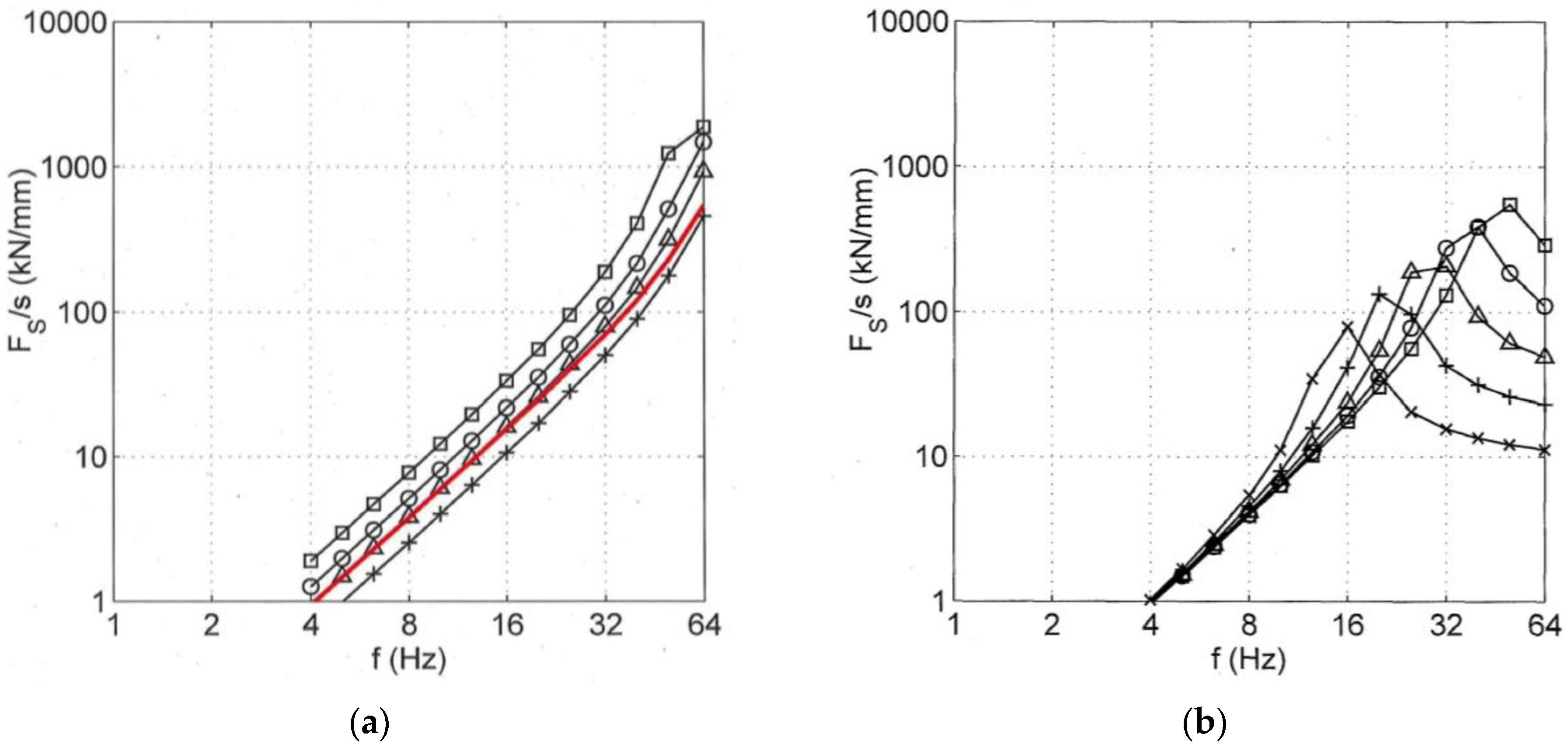
4.1. Transfer Functions of the Vehicle-Track Interaction

First, the most important vehicle–track–soil transfer function F_S/s = H_T H_V is presented for the variation of some vehicle and track parameters. The vehicle–track–soil transfer function is strongly influenced by the unsprung mass of the vehicle, the wheelset mass (Figure 4a). The dynamic axle loads are proportional to the wheelset mass for frequencies up to 64 Hz. For this frequency range, the transfer function increases strongly with F_S/s ~ f². If soft under-sleeper pads are added to the track (Figure 4b), resonances can be seen at frequencies between 16 and 64 Hz. Above these resonance frequencies, the dynamic axle-loads can be reduced to less than one-tenth of the values of a standard ballast track. Vehicle–track resonances, however, do not occur for the standard ballast track in the frequency range of interest.

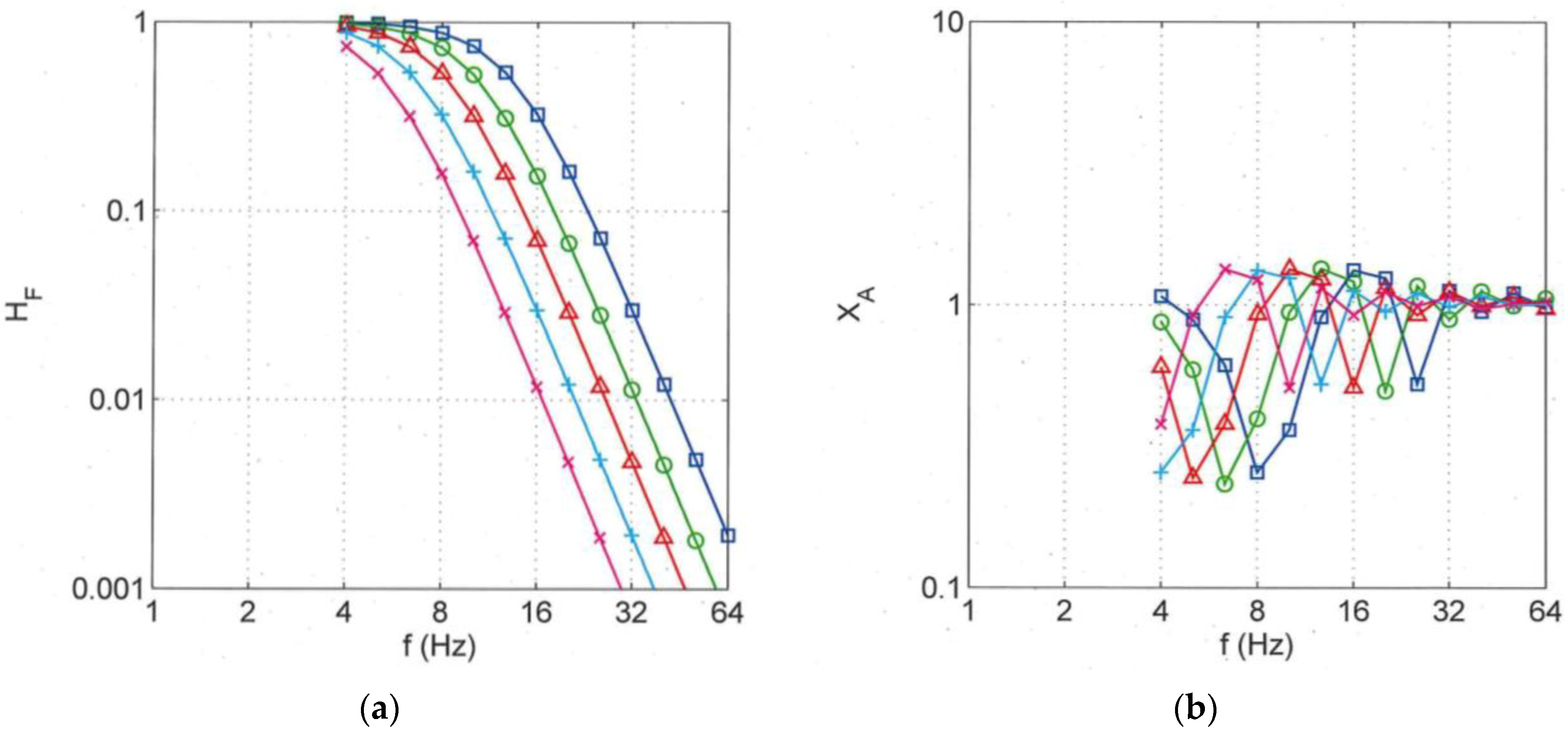
4.2. Transfer Functions of the Track Filtering

The track filtering functions for the geometric and stiffness-induced track support irregularities are shown in Figure 5. Figure 5a shows that the low-frequency geometric track support irregularity s_S is passed directly through the track to give the rail irregularity s_R, yielding a transfer value of s_R/s_S = 1. Frequencies higher than 12 Hz (in case of a standard ballast track and train speed of v_T = 160 km/h) are reduced considerably because of a strong cut-off effect. The ballast tracks with soft sleeper pads have lower cut-off frequencies down to 8 Hz and, therefore, a stronger track filtering effect with lower effective track irregularities.

Similar observations are made for the stiffness-induced track support irregularities in Figure 5b, but the cut-off frequencies are somewhat higher, between 12 and 20 Hz, and the low-frequency transfer values depend on the stiffness of the track. The low-frequency force amplitudes are smaller for the softer sleeper pads.

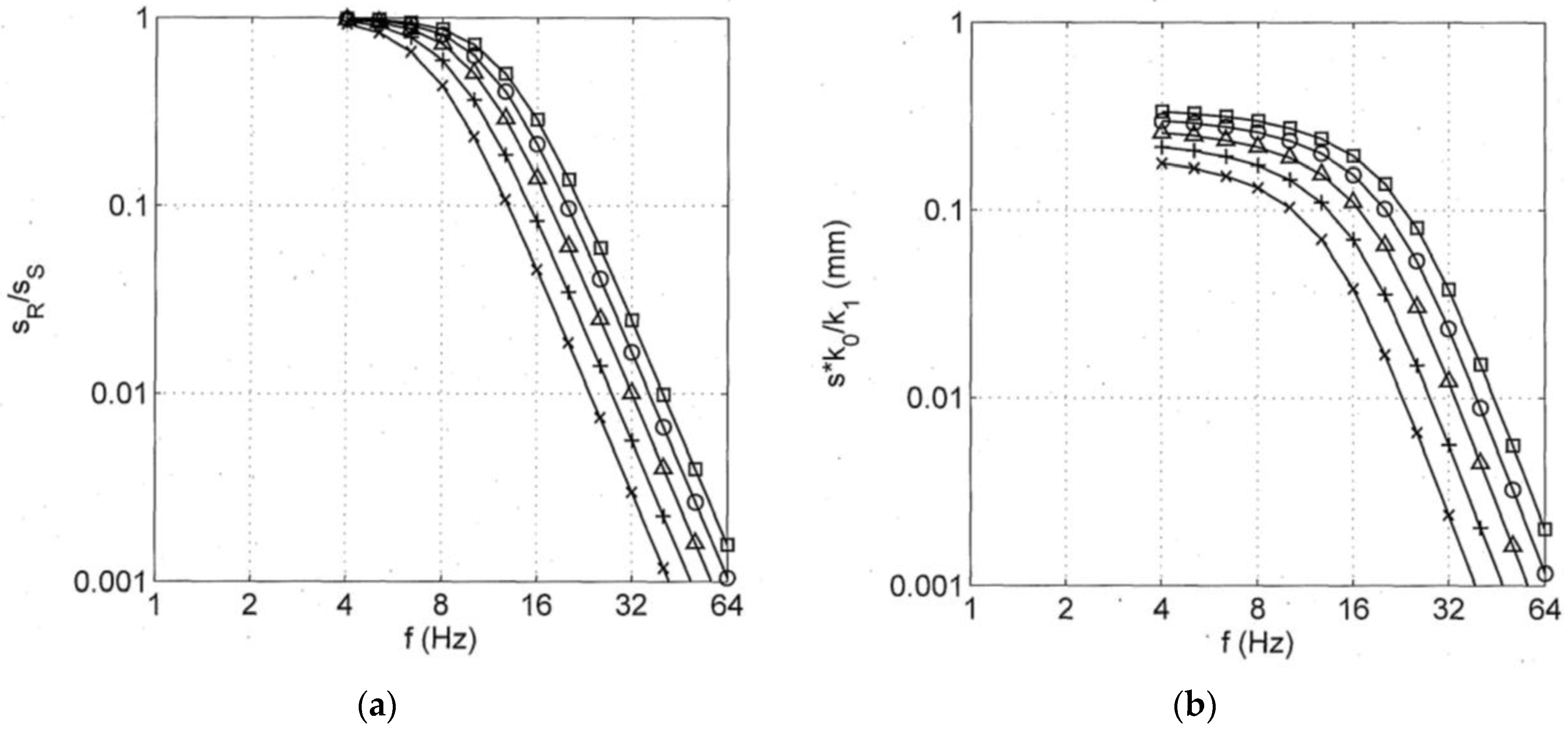
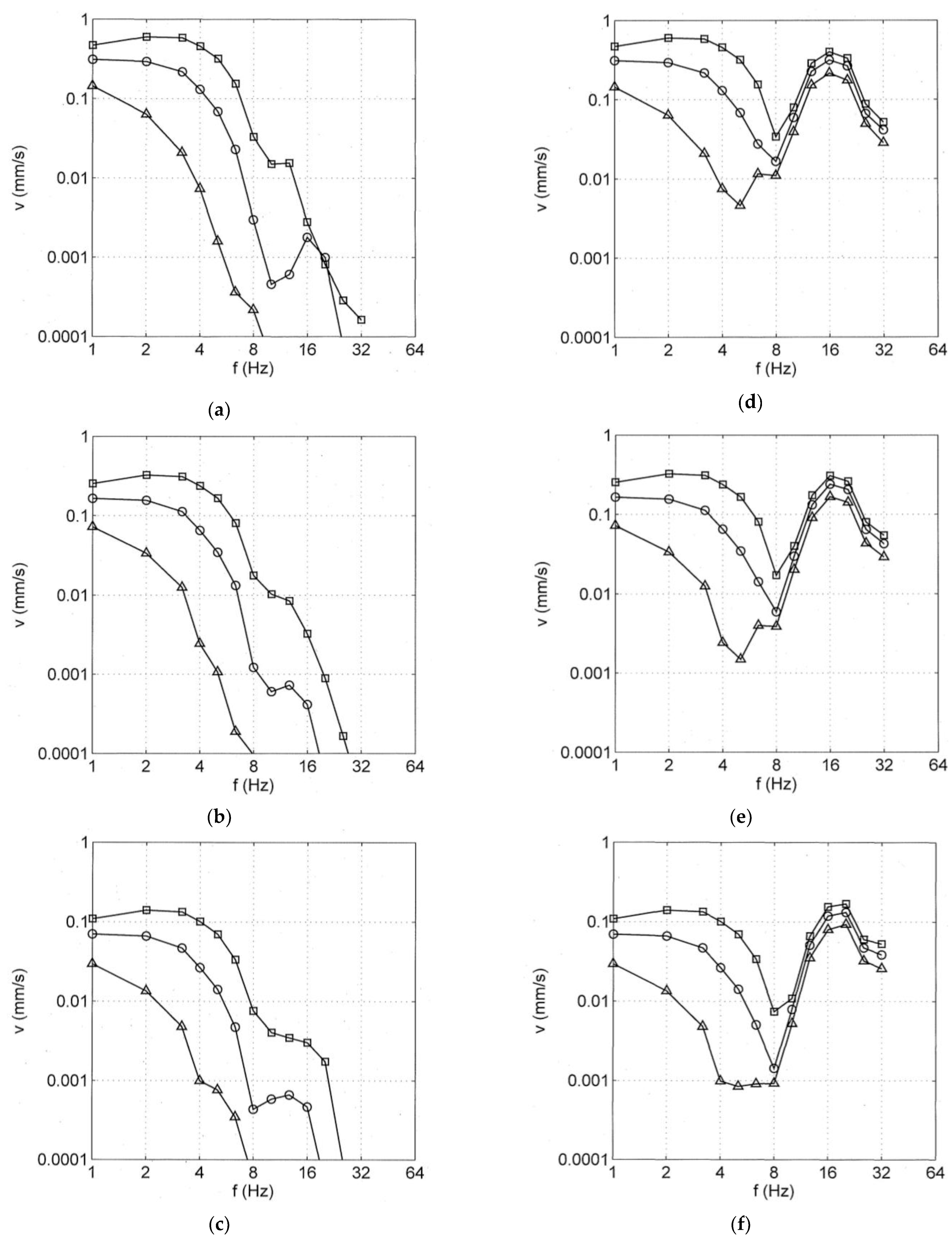
4.3. Quasi-Static Ground Response

First, the effect of the axle pulses on a regular track support is examined. A train with speed of 160 km/h and three homogeneous soils with shear wave velocities of v_S = 150, 200 and 300 m/s are considered. The train passage is presented as one-third of the octave band spectra of the particle velocity for the distances x = 3, 5, and 10 m in Figure 6a–c. The moving static loads induce very low-frequency vibrations in the neighbourhood of the railway line. The main amplitudes of this quasi-static solution are below 12 Hz at 3 m, below 6 Hz at 5 m, and below 3 Hz at 10 m. The spectra strongly decrease with frequency and with distance. This means that the regular response to the static loads is limited to the low-frequency near field of the track (see also [36,37,38]), except for trans-Rayleigh-trains in very soft soils [18]. The quasi-static ground vibration amplitudes are also reduced in a stiffer soil (Figure 6c). The typical spectra of the different distances can be used to easily identify the quasi-static component in the following calculations. In measurements, there may be some additional low-frequency maxima and minima due to special train configurations. Note that the low-frequency quasi-static solution was calculated from axle impulses of higher frequency content. The result is very similar to a calculation based on the static transfer function of the soil [37]. Obviously, the higher impulse frequencies, which come from different track points, perfectly cancel each other.

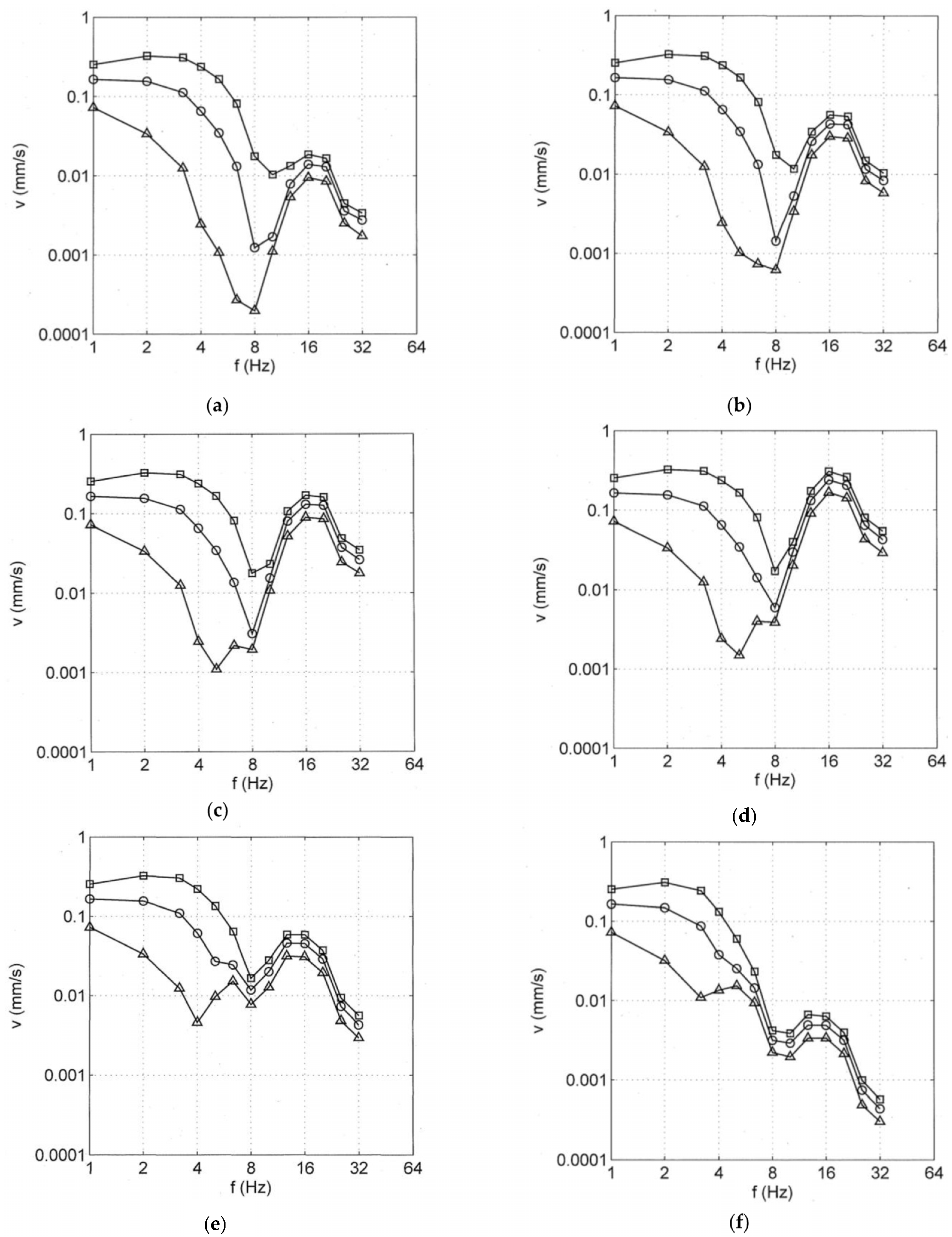
4.4. The Effect of Axle Pulses on a Randomly Varying Track Support Stiffness

Next, the train was run over an irregular track support and the ground vibration spectra are shown in Figure 6d–f. Once again, the passage of static loads generates the quasi-static response of the soil. The typical spectra can be observed below 8 Hz. For frequencies above 8 Hz, a big difference between the regular and irregular track support is obvious. Whereas the quasi-static component tends to zero, the varying track support stiffness generates a new ground vibration component with considerable amplitudes. The low-frequency quasi-static and the mid-frequency response are clearly separated by a minimum at around 8 Hz. There is a second minimum at 25 or 32 Hz, so that the mid-frequency ground vibration component can be identified by a typical maximum region between these minima. This characteristic is related to the axle-sequence spectrum X_A(f) of a bogie. The mid-frequency component also has a completely different attenuation with distance. In contrast to the strong attenuation of the quasi-static component, the mid-frequency part has a rather weak attenuation.

The mid-frequency stochastic ground vibration component is generated as follows. The static axle load runs over different excitation points of the track that have different stiffnesses. If the track is stiffer, the impulse is shorter and has a wider bandwidth. If the track is softer, the impulse is longer and the bandwidth is narrower. Therefore, low frequencies of the impulse are similar for all excitation points, but the amplitudes around the bandwidth vary considerably. The impulses from neighbouring excitation points cannot perfectly cancel each other. The remainder of the superposition constitutes the new mid-frequency ground vibration component (which is called “the scattered axle pulses”).

Figure 7a–d shows the one-third octave band spectra for q = 3, 10, 30 and 50% variation of the track support stiffness. The mid-frequency range strongly increases with the percentage of the stiffness variation. At the end for 50% variation, the mid-frequency amplitudes are as high as for the nearest quasi-static response. The stochastic mid-frequency component is only moderately higher for a softer soil (Figure 6d). Another variation in Figure 7d–f shows the influence of the track stiffness on the mid-frequency component. The bending stiffness EI of the track is increased from the rail to 10 EI and 100 EI, where 100 EI is approximately the stiffness of a 0.5 m thick concrete plate. The mid-frequency amplitudes are clearly reduced by a stiff plate, to less than one-tenth. The stiff plate results in a wider distribution of the static load along the track. This means a smoother impulse, which has lower frequencies and lower amplitudes. Thus, a new ground vibration component was found, but also a possible mitigation strategy for this component.

5. Calculated and Measured Results at a Specific Site

At a site near Würzburg, simultaneous vibration measurements of the train, the track and the soil were performed at three different track sections for different train speeds [4]. The axle-box measurements and the hammer and train-induced ground vibrations near the ballast track are used here to compare theoretical predictions with measurements.

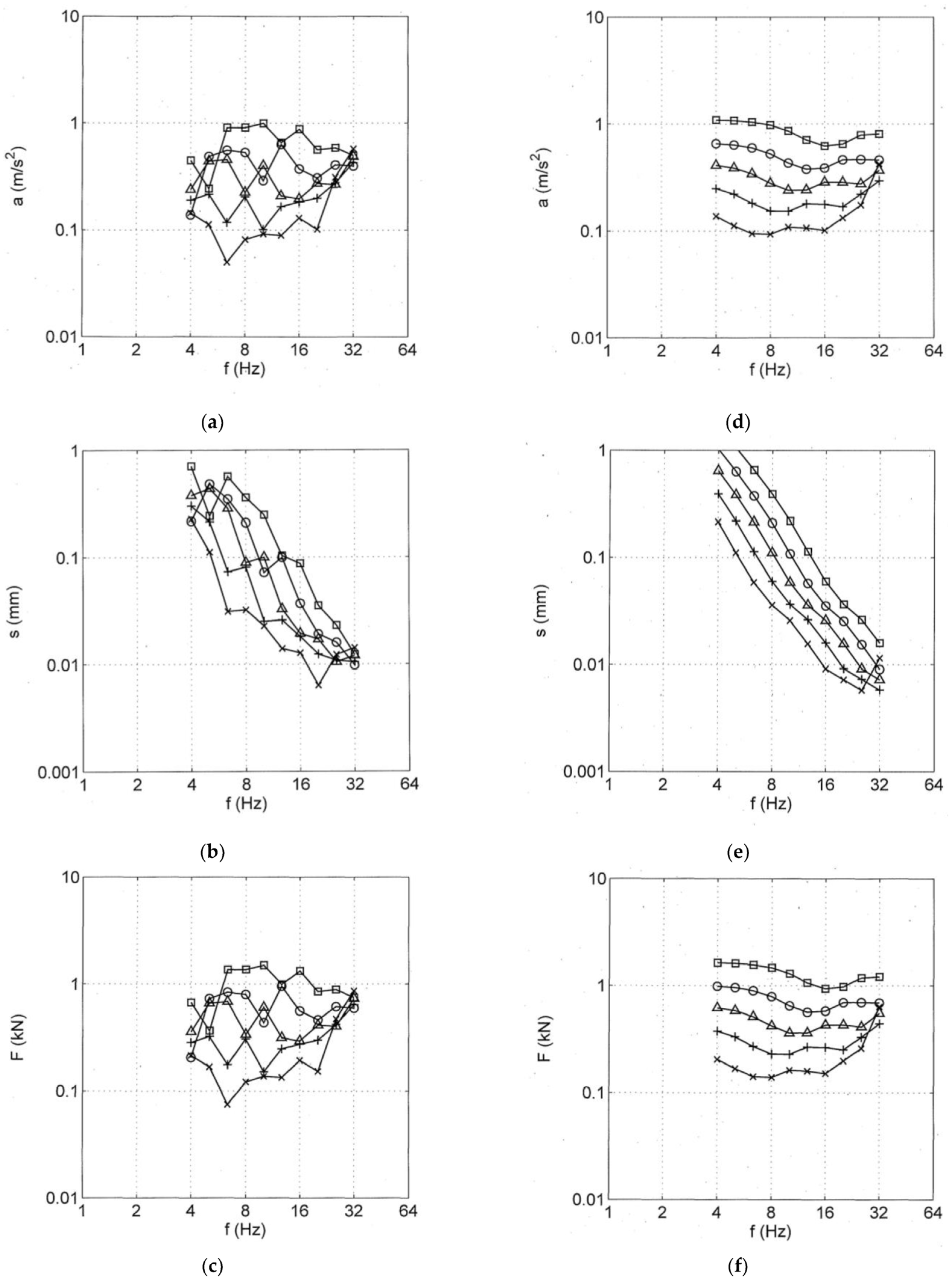
5.1. Wheelset Accelerations from Axle-Box Measurements and Corresponding Irregularities and Forces

First, the measured axle-box accelerations are shown in Figure 8a for five train speeds. The spectra are almost constant with frequency. The only exception is for the lowest speed of 63 km/h where an increase at 32 Hz can be related to the sleeper passage excitation. The accelerations are strongly increasing with train speed, and an amplitude factor of 10 is observed for train speeds between 63 and 160 km/h. Four different axle boxes were measured and all four measurement points give very similar results. Only the out of roundness at 8, 10, 12, or 16 Hz is specific for each wheel.

The measured wheelset accelerations a_W are divided by ω² to yield displacements (Figure 8b). These wheel displacements are the same as the effective irregularities s in this frequency range; see [31]. The irregularities are strongly decreasing with frequency. The accelerations a_W multiplied by the wheelset mass of m_W = 1500 kg are almost identical to the excitation forces F acting on the track (Figure 8c), with small deviations at low frequencies due to bogie contributions [31]). Therefore, the forces are almost constant with frequency and strongly increasing with train speed in the same way as the accelerations.

Corresponding results are calculated with the transfer functions of Section 3.2 and the following irregularities s_S of the subground and s_W the combined unevenness of wheel and rail:

$$\begin{gathered} s_S=s_{S1}{\left(\lambda /{\lambda }_1\right)}^2 \mathrm{with} s_{S1}=0.02 \mathrm{mm} \mathrm{at} {\lambda }_1=1.2 \mathrm{m} \\ {s}_W=s_{W1}\left(\lambda /{\lambda }_1\right) \mathrm{with} s_{W1}=0.01 \mathrm{mm} \mathrm{at} {\lambda }_1=1.2 \mathrm{m} \end{gathered}$$

(26)

The stiffness variation is assumed to be constant at k₁/k₀ = 20%, and the stiffness variation by the sleeper passage is included as an effective irregularity of s_D = 0.012 mm. The resulting effective irregularity at rail level is shown in Figure 8e. For the train speed of 100 km/h (curve ∆), the following components can be observed. At low frequencies, the geometric track support irregularities dominate, but also strongly decrease with s_R ~ f⁻². The transfer function H_sT for the geometrical track support irregularity has a cut-off at about 8 Hz and, therefore, the effective irregularity s* from the support stiffness variation dominates at about 12 Hz. This component is initially constant with frequency and the cut-off of the corresponding transfer function H_kT is at about 20 Hz, from where the stiffness component also decreases until the wheel and track unevenness s_W is dominant at 25 Hz.

In the next step, the decreasing irregularities have to be multiplied by the increasing vehicle–track transfer functions (6) and (7). The resulting axle-load spectra in Figure 8f are almost constant with frequency. The amplitudes increase with increasing train speed as F~v_T². The dynamic load is about F ≈ 0.4 kN for 100 km/h and reaches F ≈ 1.0 kN for 160 km/h.

The measurements and calculations of the train–track interaction are in good agreement in all details: the irregularities are strongly decreasing with frequency, and the accelerations and forces are constant in frequency and strongly increasing with train speed A~v_T², and have the same amplitude of 1.0 kN for 160 km/h.

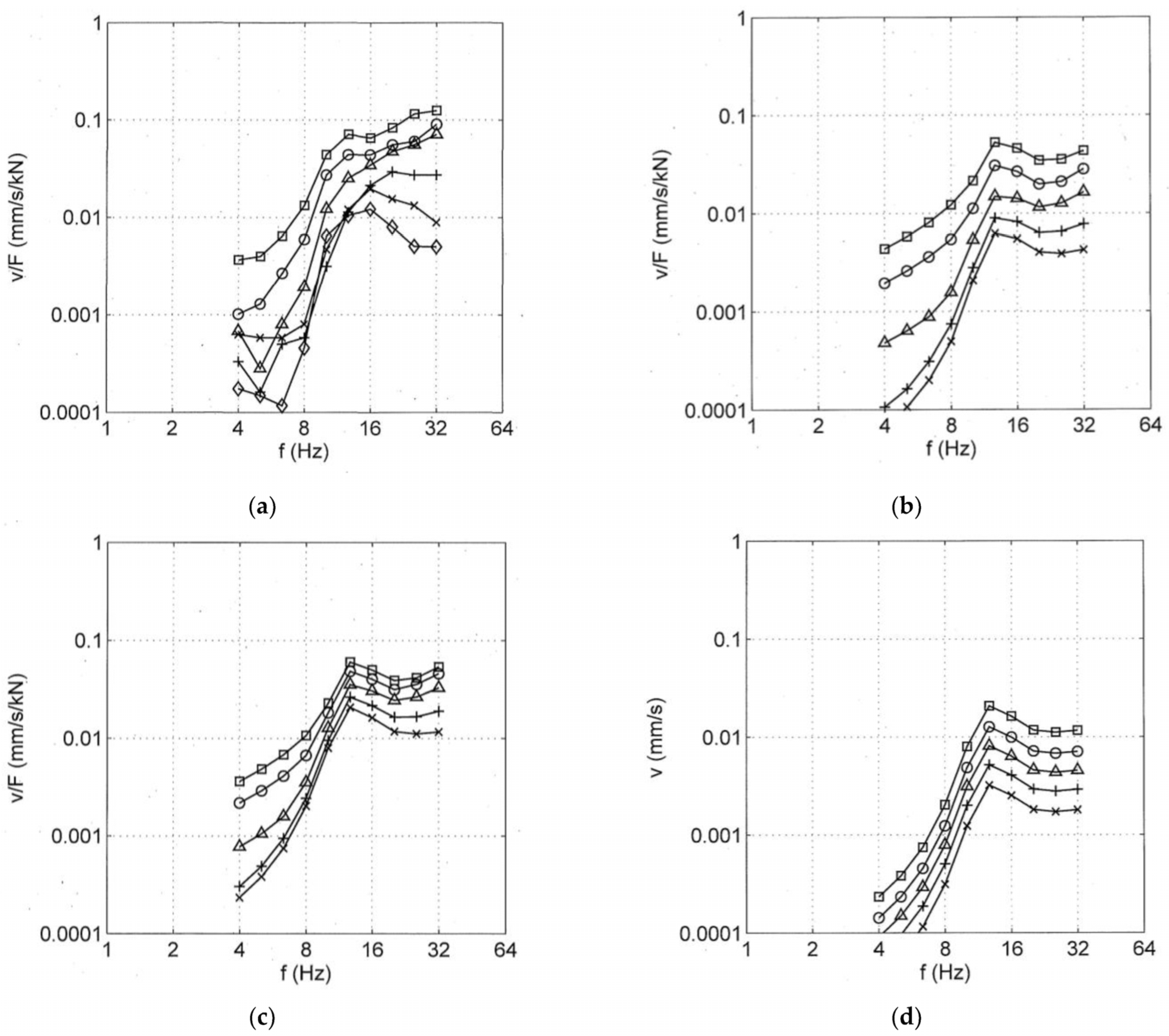
5.2. Measured and Calculated Transfer Functions of the Soil

The transfer functions of the soil at this site were measured by hammer impacts and sensor distances between 3 and 30 m (Figure 9a). A soil model was fitted to these transfer functions, which consists of a layer of height h = 11 m, a shear wave velocity v_S1 = 270 m/s and an underlying half-space of v_S2 = 1000 m/s. The theoretical transfer functions of this layered situation are presented in Figure 9b, which show all the same characteristics as the measured transfer functions. The low-frequency amplitudes are small because of the stiff half-space, whereas the high frequencies have the greater amplitudes of the softer layer. Between these two different amplitude ranges, a strong increase in amplitudes can be found, which is followed by a moderate resonance at 12.5 Hz.

The transfer functions in Figure 9a,b hold for a point load. A number of point loads of a 1 kN amplitude per axle and one-third octave band were superposed stochastically to obtain the transfer function for a train load (the response to a standard train load, Figure 9c). The characteristics are the same as for the point load. The near field has almost the same amplitude, whereas the far field of the train load has higher amplitudes. This leads to a weaker attenuation with distance and a narrower band of transfer functions.

Another representation is given for the results at a 30 m distance. Figure 9d shows the spectra for different train speeds v_T, which are calculated by different dynamic loads of F = 0.155 to 1.0 kN per axle and one-third octave band. The curves are regularly shifted vertically upwards proportional to the dynamic axle load.

5.3. Ground Vibrations from Static or Dynamic Axle Loads and from Measurement

Now the ground vibrations from train passages are predicted and compared with the measurements. The response at different distances from the track (for a train speed of 160 km/h) and the response for different train speeds (at a distance of 30 m) are shown in Figure 10. Theoretical responses are shown for the dynamic loads from irregularities in Figure 10a,b and for the static loads on a varying track support. In addition to the transfer functions H_S of the layered soil, the axle sequence X_A Equation (22) of the bogies is included in both cases.

The wave field for the dynamic loads (Figure 10a) is very similar to the transfer functions in Figure 9c, as the dynamic loads are (almost) constant and at 1 kN for 160 km/h. In addition to the characteristics of the layered soil, the maximum at 12.5 Hz is increased slightly because of the axle sequence spectrum. The different train speeds (Figure 10b) have different axle sequence spectra, so that the regular pattern of Figure 9d is lost. The strict order of the train speeds can only be found at the highest frequencies. A clear maximum occurs only for 125 and 160 km/h.

The measured train-induced wave field (Figure 10c) shows the small low-frequency amplitudes of the deeper stiff soil and the strong increase at about 10 Hz. The maximum at 12.5 Hz is more pronounced than for the transfer functions (Figure 9c) as the curves of all distances come close together. The high-frequency amplitudes are approximately those of the upper layer. The curves of different train speeds (Figure 10d) show clearly elevated responses for 125 and 160 km/h, whereas the train speeds below 100 km/h induce only smaller ground vibrations. The ground vibrations from dynamic loads in Figure 10a and b are clearly smaller than (less than half) the ground vibration from measurements in Figure 10c,d.

The ground vibrations from the static loads are presented in Figure 10e,f. In the near field, the quasi-static component can be found between 4 and 6 Hz. All other amplitudes are the result of the varying track support stiffness. The maxima at 12.5 Hz are increased by the pulses of the static axle loads, and they are much higher than for the dynamic loads in Figure 10a,b. The minima are almost at the same frequencies (8 Hz and 20/25 Hz) for the static loads, the dynamic loads and the measurements. The minima are strongest for the static pulse loads, which have an extra reduction in addition to the minima from the axle sequence and the low frequency reduction in the layering. The maximum, on the other hand, is increased by the static pulse loads in addition to the nearby (moderate) maxima of the axle sequence and the resonance of the layering. Because of these effects, the static loads yield the highest near-field amplitudes at 12.5 Hz, and at 30 m, they generate a maximum (Figure 10f), which is clearly higher than the maximum of the dynamic loads (Figure 10b) and nearly reaches the amplitude of the measurements (Figure 10d).

These measured and calculated results show that the elevated mid-frequency vibrations can be better explained by the randomly varying track support than by the dynamic loads from the irregularities. The importance of the axle pulses on an irregular track and soil (the scattering of axle pulses) for the ground vibration near railway lines was indicated by more experimental results of BAM [31,37,39], and in [40] measurements of other researchers were re-sampled and collected from, for example, [14,17,19,41,42].

6. Conclusions

The excitation of ground vibrations by different irregularities of the railway track was analysed, considering the widely used geometric irregularities at the wheel–rail contact, stiffness irregularities, irregularities from different track positions and irregularities in the wave propagation. Formulas were given in the frequency-wavenumber domain, and example transfer functions (the force on the soil related to the specific irregularity) were calculated. The transfer functions show the increasing influence of the wheelset mass and the reducing influence of soft track elements (e.g., sleeper pads). The latter yield cut-off frequencies of 8 to 16 Hz and resonance frequencies of 16 to 50 Hz. Whereas most irregularities generate dynamic axle loads, static (gravity-induced) loads of the vehicle have some special effects. The static loads are moving constant loads, which were calculated as the very low-frequency quasi-static component of the near-field ground vibration. In the case where the track support stiffness varies randomly along the track, the results for the moving constant loads were calculated by the frequency-domain superposition of axle pulses and a stochastic simulation. This computation yields, in addition to the regular quasi-static component, a strong stochastic mid-frequency component because of the “scatter” of the axle pulses.

Experimental results of simultaneous vehicle, track and soil measurements were presented and compared with the theoretical results for the dynamic and static loads. Effective track irregularities, dynamic axle loads and ground vibration at different distances and for different train speeds were analysed. It was found that the dynamic loads that are evaluated from the measured axle-box accelerations are not great enough to generate the measured ground vibrations. The stochastic component of the moving static load, however, can generate the higher measured ground vibration amplitudes. This indicates that a static load moving over a varying track support stiffness can produce an important ground vibration component by the scatter of axle pulses.

References

1. Berawi, A. Improving Railway Track Maintenance Using Power Spectral Density (PSD). Ph.D. Thesis, University of Porto, Porto, Potrugal, 2013. [Google Scholar]
2. Hamid, A.; Rasmussen, K.; Baluja, M.; Yang, T. Analytical Description of Track Geometry Variations; Report for Federal Railroad Administration; ENSCO Inc.: Springfield, IL, USA, 1983. [Google Scholar]
3. Esveld, C. Modern Railway Track; MRT-Productions: Duisburg, Germany, 1989. [Google Scholar]
4. Auersch, L. Simultaneous measurements of the vehicle, track, and soil vibrations at a surface, bridge, and tunnel railway line. Shock. Vib. 2017, 2017, 1959286. [Google Scholar] [CrossRef] [Green Version]
5. Takemiya, H. Ground vibrations alongside tracks induced by high-speed trains: Prediction and mitigation. In Noise and Vibration from High-Speed Trains; Krylov, V., Ed.; Thomas Telford: London, UK, 2001; pp. 347–391. [Google Scholar]
6. Sheng, X.; Jones, C.; Thompson, D. A theoretical model for ground vibration from trains generated by vertical track irregularities. J. Sound Vib. 2004, 272, 937–965. [Google Scholar] [CrossRef]
7. Lombaert, G.; Degrande, G.; Kogut, J.; François, S. The experimental validation of a numerical model for the prediction of railway induced vibrations. J. Sound Vib. 2006, 297, 512–535. [Google Scholar] [CrossRef]
8. Maldonado, M. Vibrations Dues au Passage d’un Tramway—Mesures Expérimentales et Simulations Numériques. Ph.D. Thesis, Ecole Centrale de Nantes, Nantes, France, 2009. [Google Scholar]
9. Ju, S.; Lin, H. Experimentally investigating finite element accuracy for ground vibrations induced by high-speed trains. Eng. Struct. 2008, 30, 733–746. [Google Scholar] [CrossRef]
10. Kouroussis, G. Modélisation des Effets Vibratoirs du Traffic Ferroviaire sur L’environnement. Ph.D. Thesis, University of Mons, Mons, Belgium, 2009. [Google Scholar]
11. Connolly, D. Ground Borne Vibrations from High-Speed Trains. Ph.D. Thesis, University of Edinburgh, Edinburgh, UK, 2013. [Google Scholar]
12. Ekevid, T.; Wiberg, N. Wave propagation related to high-speed train: A scaled boundary FE-approach for unbounded domains. Comput. Methods Appl. Mech. Eng. 2002, 191, 3947–3964. [Google Scholar] [CrossRef]
13. Galvin, P.; Dominguez, J. Experimental and numerical analyses of vibrations induced by high-speed trains on the Cordoba-Malaga line. Soil Dyn. Earthq. Eng. 2009, 29, 641–657. [Google Scholar] [CrossRef]
14. Romero, A. Predicción, Medida Experimental y Evaluación de las Vibraciones Producidas por el Tráfico Ferroviario. Ph.D. Thesis, University of Sevilla, Sevilla, Spain, 2012. [Google Scholar]
15. Yang, Y.; Hung, H. A 2.5D finite/infinite finite element approach for modelling viscoelastic bodies subjected to moving loads. Int. J. Numer. Methods Eng. 2001, 51, 1317–1336. [Google Scholar] [CrossRef]
16. Galvin, P.; Francois, S.; Schevenels, M.; Bongini, E.; Degrande, G.; Lombaert, G. A 2.5D coupled FE-BE model for the prediction of railway induced vibrations. Soil Dyn. Earthq. Eng. 2010, 30, 1500–1512. [Google Scholar] [CrossRef] [Green Version]
17. Alves Costa, P. Vibrações do Sistema Via-Maciço Induzidas por Tráfego Ferroviário—Modelação Numérica e Validação Experimental. Ph.D. Thesis, University of Porto, Porto, Portugal, 2011. [Google Scholar]
18. Krylov, V. Ground vibration boom from high-speed trains: Prediction and reality. Acoust. Bull. 1998, 23, 15–22. [Google Scholar]
19. Triepaischajonsak, N.; Thompson, D.; Jones, C.; Ryue, J.; Priest, J. Ground vibration from trains: Experimental parameter characterisation and validation of a numerical model. Rail Rapid Transp. 2011, 225, 140–153. [Google Scholar] [CrossRef]
20. Auersch, L. Theoretical and experimental excitation force spectra for railway induced ground vibration—Vehicle-track soil interaction, irregularities and soil measurements. Veh. Syst. Dyn. 2010, 48, 235–261. [Google Scholar] [CrossRef]
21. Verheijen, E. A survey on roughness measurement. J. Sound Vib. 2006, 293, 784–794. [Google Scholar] [CrossRef]
22. Johansson, A. Out-of-Round Railway Wheels—Literature Survey, Field Tests and Numerical Simulations. Ph.D. Thesis, University of Göteborg, Gothenburg, Sweden, 2003. [Google Scholar]
23. Hunt, H. Types of rail roughness and the selection of vibration isolation measures. In Noise and Vibration Mitigation for Rail Transportation Systems; Notes on Numerical Fluid Mechanics and Multidisciplinary Design; Springer: Berlin/Heidelberg, Germany, 2008; Volume 99, pp. 341–347. [Google Scholar]
24. Auersch, L. Excitation of ground vibration due to the passage of trains over a track with trackbed irregularities and a varying support stiffness. Veh. Syst. Dyn. 2015, 53, 1–29. [Google Scholar] [CrossRef]
25. Verachtert, R.; Hunt, H.; Hussein, M.; Degrande, G. Changes of perceived unevenness by in-track vibration countermeasures in slab track. Eur. J. Mech. A/Solids 2017, 65, 40–58. [Google Scholar] [CrossRef]
26. Auersch, L. Parametric excitation of rail-wheel-system: Calculation of vehicle–track–subsoil-dynamics and experimental results of the high-speed train Intercity experimental. Arch. Appl. Mech. 1990, 60, 141–156. (In German) [Google Scholar]
27. Nielsen, J.; Igeland, A. Vertical dynamic interaction between train and track—Influence of wheel and track imperfections. J. Sound Vib. 1995, 187, 825–839. [Google Scholar] [CrossRef]
28. Fröhling, R. Deterioration of Railway Track Due to Dynamic Vehicle Loading and Spatially Varying Track Stiffness. Ph.D. Thesis, University of Pretoria, Pretoria, South Africa, 1997. [Google Scholar]
29. Oscarsson, J. Dynamic train-track interaction: Variability attributable to scatter in the track properties. Veh. Syst. Dyn. 2002, 37, 59–79. [Google Scholar] [CrossRef]
30. Berggren, E. Railway Track Stiffness—Dynamic Measurements and Evaluation for Efficient Maintenance. Ph.D. Thesis, KTH Stockholm, Stockholm, Sweden, 2009. [Google Scholar]
31. Auersch, L. The role of vehicle dynamics in train-induced ground vibrations and the detection of irregular axle-pulse responses due to a varying track stiffness. Rail Rapid Transit 2022, 236. accepted for publication. [Google Scholar]
32. Auersch, L. Dynamics of the railway track and the underlying soil: The boundary-element solution, theoretical results and their experimental verification. Veh. Syst. Dyn. 2005, 43, 671–695. [Google Scholar] [CrossRef]
33. Auersch, L. Static and dynamic behaviours of isolated and un-isolated ballast tracks using a fast wavenumber domain method. Arch. Appl. Mech. 2017, 87, 555–574. [Google Scholar] [CrossRef]
34. Auersch, L. The excitation of ground vibration by rail traffic: Theory of vehicle–track–soil interaction and measurements on high-speed lines. J. Sound Vib. 2005, 284, 103–132. [Google Scholar] [CrossRef]
35. Auersch, L. Wave propagation in layered soil: Theoretical solution in wavenumber domain and experimental results of hammer and railway traffic excitation. J. Sound Vib. 1994, 173, 233–264. [Google Scholar] [CrossRef]
36. Sheng, X.; Jones, C.; Thompson, D. A comparison of a theoretical model for quasi-statically and dynamically induced environmental vibration from trains with measurements. J. Sound Vib. 2003, 267, 621–635. [Google Scholar] [CrossRef] [Green Version]
37. Auersch, L. Ground vibration due to railway traffic—The calculation of the effects of moving static loads and their experimental verification. J. Sound Vib. 2006, 293, 599–610. [Google Scholar] [CrossRef]
38. Lombaert, G.; Degrande, G. Ground-borne vibration due to static and dynamic axle loads of InterCity and high-speed trains. J. Sound Vib. 2009, 319, 1036–1066. [Google Scholar] [CrossRef]
39. Auersch, L. Train induced ground vibrations: Different amplitude-speed relations for two layered soils. J. Rail Rapid Transit 2012, 226, 469–488. [Google Scholar] [CrossRef]
40. Auersch, L. Fast trains and isolating tracks on inhomogeneous soils. In Ground Vibrations from High-Speed Railways: Prediction and Mitigation; Krylov, V., Ed.; ICE Publishing: London, UK, 2019; pp. 27–76. [Google Scholar]
41. Degrande, G.; Schillemanns, L. Free field vibrations during the passage of a Thalys high-speed train at variable speed. J. Sound Vib. 2001, 247, 131–144. [Google Scholar] [CrossRef] [Green Version]
42. Zhai, W.; Wei, K.; Song, X.; Shao, M. Experimental investigation into ground vibrations induced by very high speed trains on a non-ballasted track. Soil Dyn. Earthq. Eng. 2015, 72, 24–36. [Google Scholar] [CrossRef] [Green Version]
Figure 1. Train induced ground vibration, (a) at site N, (b) at site H, at distances x = □ 3, ○ 5, ∆ 10, + 20, × 30, and ◊ 50 m [20].
Applsci 12 01463 g001
Figure 2. Track model consisting of rail, rail pad, sleeper, sleeper pad, ballast, ballast mat, ballast plate and continuous soil.
Applsci 12 01463 g002
Figure 3. Spectra for the calculation of a standard ballast track with varying track support stiffness, (a) filter function of the track force, (b) axle-sequence spectrum of two axles of a bogie, train speed × 63, + 80, ∆ 100, ○ 125, and □ 160 km/h.
Applsci 12 01463 g003
Figure 4. Transfer functions of vehicle–track interaction (dynamic axle loads due to irregularities) (a) for different wheelset masses mW = + 1000, ∆ 1500, ○ 2000, and □ 3000 kg, 1500 kg with HT(f) = 1, and (b) for different under-sleeper pads with stiffness of kP = × 10, + 20, ∆ 40, ○ 80, and □ 160 × 106 N/m.
Applsci 12 01463 g004
Figure 5. Transfer functions for the track filtering (a) of geometric track bed errors, and (b) of a stiffness variation, ballast tracks with different under-sleeper pads with stiffness of kP = × 10, + 20, ∆ 40, ○ 80, and □ 160 106 N/m.
Applsci 12 01463 g005
Figure 6. Train passage with vT = 160 km/h over a regular (a,c,e) and an irregular ballast track (b,d,f), q = 50%), different soils with vS = (a,b) 150, (c,d) 200, (e,f) 300 m/s, one-third of the octave band spectrum at distances x = □ 3, ○ 5, ∆ 10 m.
Applsci 12 01463 g006
Figure 7. Train passage with vT = 160 km/h over an irregular track and a soil with vS = 200 m/s, irregularity q = (a) 3%, (b) 10%, (c) 30%, (df) 50%, track stiffness (ad) EI ballast track, (e) 10 EI, (f) 100 EI slab track, one-third of the octave band spectrum at distances x = □ 3, ○ 5, ∆ 10 m.
Applsci 12 01463 g007
Figure 8. Measured (ac) and calculated (df) vehicle–track interactions at site W for train speeds vT = □ 160, ○ 125, ∆ 100, + 80, and × 63 km/h; wheelset acceleration (a,d), effective irregularities (b,e), dynamic axle loads (c,f).
Applsci 12 01463 g008
Figure 9. Transfer functions for the soil at site W, distances x = □ 3, ○ 5, ∆ 10, + 20, × 30 m, (a) measured from hammer impact, (b) calculated for a point load, (c) calculated for a standard train load; (d) response to constant train loads between 0.15 and 1 kN per one-third octave band representing train speeds of vT = □ 160, ○ 125, ∆ 100, + 80, and × 63 km/h.
Applsci 12 01463 g009
Figure 10. Comparison of measured and calculated ground vibrations; wavefield at distances x = □ 3, ○ 5, ∆ 10, + 20, × 30 m for the maximum train speed of 160 km/h (a,c,e), and for different train speeds of vT = □ 160, ○ 125, ∆ 100, + 80, × 63 km/h at a distance of 30 m (b,d,f), calculated with geometric track irregularities (a,b), measured at site W (c,d), and calculated by a varying track support stiffness (e,f).
Applsci 12 01463 g010
Publisher’s Note: MDPI stays neutral with regard to jurisdictional claims in published maps and institutional affiliations.