Article

Psychological Stress Level Detection Based on Heartbeat Mode

1
Institute of Intelligent Machines, Hefei Institutes of Physical Science, Chinese Academy of Sciences, Hefei 230031, China
2
Department of Science Island, University of Science and Technology of China, Hefei 230026, China
*
Author to whom correspondence should be addressed.
Appl. Sci. 2022, 12(3), 1409; https://doi.org/10.3390/app12031409
Submission received: 23 November 2021 / Revised: 24 January 2022 / Accepted: 26 January 2022 / Published: 28 January 2022

Abstract

:
The effective detection and quantification of mental health has always been an important research topic. Heart rate variability (HRV) analysis is a useful tool for detecting psychological stress levels. However, there is no consensus on the optimal HRV metrics in psychological assessments. This study proposes an HRV analysis method that is based on heartbeat modes to detect drivers’ stress. We used statistical tools for linguistics to detect and quantify the structure of the heart rate time series and summarized different heartbeat modes in the time series. Based on the k-nearest neighbors (k-NN) classification algorithm, the probability of each heartbeat mode was used as a feature to detect and recognize stress caused by the driving environment. The results indicated that the stress from the driving environment changed the heartbeat mode. Stress-related heartbeat modes were determined, facilitating detection of the stress state with an accuracy of 93.7%. We also concluded that the heartbeat mode was correlated to the galvanic skin response (GSR) signal, reflecting real-time abnormal mood fluctuations. The proposed method revealed HRV characteristics that made quantifying and detecting different mental conditions possible. Thus, it would be feasible to achieve personalized analyses to further study the interaction between physiology and psychology.

1. Introduction

Human health is closely related to mental stress, which is subjective and continuously variable. Thus, determining the onset, duration, and severity of stressful events is a difficult and worthy research topic [1,2]. Furthermore, it is a challenging task for researchers and clinicians to obtain biomarkers of stress and health [3].
Stress may lead to dynamic changes in the autonomic nervous system (ANS), which are characterized by an increase in sympathetic nervous system (SNS) activity and a decrease in parasympathetic nervous system (PNS) activity [4]. Heart-rate variability (HRV) features are considered to be viable physiological markers for evaluating ANS activity when detecting stress [5,6]. HRV represents the changes in the time intervals between consecutive heartbeats, which can easily be extracted from electrocardiograph (ECG) signals [7].
Heart rate (HR) is controlled by the balancing action of the SNS and PNS branches [8]. The relative increase in sympathetic activity is related to an increase in heart rate, and the relative increase in parasympathetic activity is related to a decrease in heart rate [4,8]. Sympathetic effects are slow, on the time scale of seconds, whereas parasympathetic effects are fast, on the time scale of milliseconds [4]. Sympathetic effects can produce rapid changes in the heartbeat interval, and these changes have significant individual differences [4,9]. Therefore, the ideal HRV index for stress detection must reveal the change rule of the heartbeat interval at the shortest time scale while adapting to individual differences.
Over the past two decades, several HRV analysis methods (e.g., time-based, frequency-based, and nonlinear measures) have been used to detect psychological stress levels [7,10]. In terms of psychological aspects, there is no clear consensus on optimal HRV metrics, and many indicators are highly correlated, resulting in a lack of interpretation clarity [7,11,12,13]. Another major problem with HRV measurement is that there are significant differences between individuals, and these differences are usually only visible at the group level [13,14,15].
McCraty et al. [16] analyzed the HRV power spectrum caused by different emotions and found that positive emotions (e.g., appreciation and compassion) are related to a more coherent heart-rhythm pattern, whereas negative emotions (e.g., stress) can negatively impact the coherence of heart-rhythm patterns [16]. McCraty et al. [16] proposed a model of psychophysiological coherence in which different emotions are reflected in specific heart-rhythm patterns independent of HRV values. However, frequency domain analysis relies on longer data (usually 5 min) and is greatly affected by abnormal normal-to-normal interval (NNI) values caused by false detection [10,11]. Dalmeida et al. [6] showed that HRV time-domain metrics (e.g., average of NNIs (avNN), standard deviation of the average NNIs (SDNN), and root mean-square differences of successive NNIs (RMSSD) are important features for stress detection. Pereira et al. [17] used a short time window to study various heart-rate variability indicators for stress-level assessment and proved that time-domain analysis is the most robust stress detection method. They used the four-stage Trier Social Stress Test (TSST) as a stress-inducing protocol in which the avNN metric allows fine-grained analysis of stress effects; it is the most reliable metric for identifying stress levels [17,18].
Despite the vast amount of literature on HRV analysis and its application potential to the design of a stress index, a standard stress index based on ANS assessment does not exist [9]. Hence, we propose an HRV analysis method based on heartbeat mode to evaluate the dynamic changes in ANS under stress.
In this study, statistical tools typically used in linguistics were used to detect and quantify heart-rate time-series structures. We focused on the variation between heartbeat intervals and ignored the values of the interval itself. This method can reveal the variation rule of heart-rate variability in a shorter time scale (m + 1 NNIs; in this study, m = 4), which is less affected by the abnormal NNI value caused by false detection. The different beating modes (bms) in the time series were summarized, and the specific bm related to different individuals’ stress was obtained. Based on the k-nearest neighbor (k-NN) algorithm used for classification, the frequency of bm (bmNN) was used as a feature to detect and recognize stress. We verified the feasibility of the method by comparing the recognition accuracy of bmNN and the classical avNN index in the public driving stress database. We also eliminated the impact of abnormal events during the rest period in the driving stress database by observing the galvanic skin response (GSR) signal waveform to improve the overall accuracy of stress assessment.
This paper is organized as follows. The proposed stress-level assessment approach based on heartbeat mode is described in Section 2. Section 3 explains the findings of this research and compares them with the classical avNN index. Section 4 discusses the achieved results and compares them to previous stress detection methods, and Section 5 summarizes the paper.

2. Heartbeat Mode-Based Stress Detection Algorithm

Before introducing the proposed heartbeat mode-based stress detection algorithm, we discuss the drivedb database provided by Healey et al. [19] for PhysioNet [20], as it pertains to our recognition strategy.

2.1. Drivedb Database and Recognition Strategy

2.1.1. Drivedb Database

The drivedb database contains a set of multiple physiological recordings (e.g., ECG, electromyography (EMG), gastrocsoleus recession (GSR) of foot, GSR of hand, and respiratory data) of healthy subjects from when they were driving along designated routes in Boston and surrounding areas. The experimental design consisted of video information and questionnaires used to assess stress levels during real-time driving [19]. The data indicate that rest time, highway, and city driving scenes caused low, medium, and high stress levels, respectively, as identified by driver physiological characteristics [19,21].
In this study, only ECG signals were used to detect and classify stress. The influence of abnormal mood fluctuations on classification results was analyzed and interpreted while referring to the waveform changes of the GSR signals. The database contains 17 public driving datasets. Among these, three (i.e., Drive01, Drive03, and Drive17) did not have complete markings of the driving environment. Drive05 lacked the ECG information for the first highway section, Drive09 and Drive16 lacked markings for the final rest times, and Drive14 and Drive13 contained repeated ECG signals that had to be discarded. The remaining 10 driving datasets were used.
Marker signals were sets of time markers that the experimenter recorded at the beginning of different driving sections. Each driving dataset was segmented into six driving sections based on environmental markers and GSR signals. The sections were separated by a buffer of 50–200 s as the stress level transitioned, during which ECG data were not analyzed. Table 1 shows how the times after the 10 driving datasets were divided into driving sections. Figure 1 shows an example of the ECG, GSR, and marker signals of Drive08 in the drivedb database. The entire process included six driving periods: Rest1, City1, Hwy1, Hwy2, City2, and Rest2.

2.1.2. Recognition Strategy

Since the experiment was carried out on actual roads, the events encountered by the drivers were uncontrollable, making it difficult to distinguish between the stresses caused by driving tasks on the highway and the city [19]. This was further complicated by the fact that the driving time on the highway was short (e.g., the driving time on Hwy2 in Drive04 was 200 s, and only five samples could be generated), and the data for each driving dataset were limited. Unlike previous studies of stress detection based on the drivedb database that used all driving datasets as training samples, we only required a single dataset for training to detect stress. In this study, the k-NN classification algorithm was used to classify two kinds of stress (rest/driving) to determine the bms most related to driving stress. We mainly analyzed the results of the two categories (rest/driving) by comparing the bmNN feature with the avNN feature.
Furthermore, the driver was not completely stress-free during rest, as the initial discomfort of wearing the sensor, boredom, and anticipation of the beginning or end of the experiment likely affected their mental states [19]. This phenomenon greatly affects the authenticity of the classification results. Healey et al. [19] reported that the driver was agitated during rest as he needed to use the bathroom, causing obvious fluctuations in the GSR waveform.
The GSR represented changes in sweat-gland activity, which reflected the intensity of the subject’s emotional state [21,22,23]. As the stress level of the driving environment changed, the activity of the sweat glands changed accordingly. Increased skin conductivity reflects high stress, while decreased conductivity indicates low stress [21,23]. Healey et al. [19,23] proved that GSR is related to driving stress and provides optimal real-time correlations.
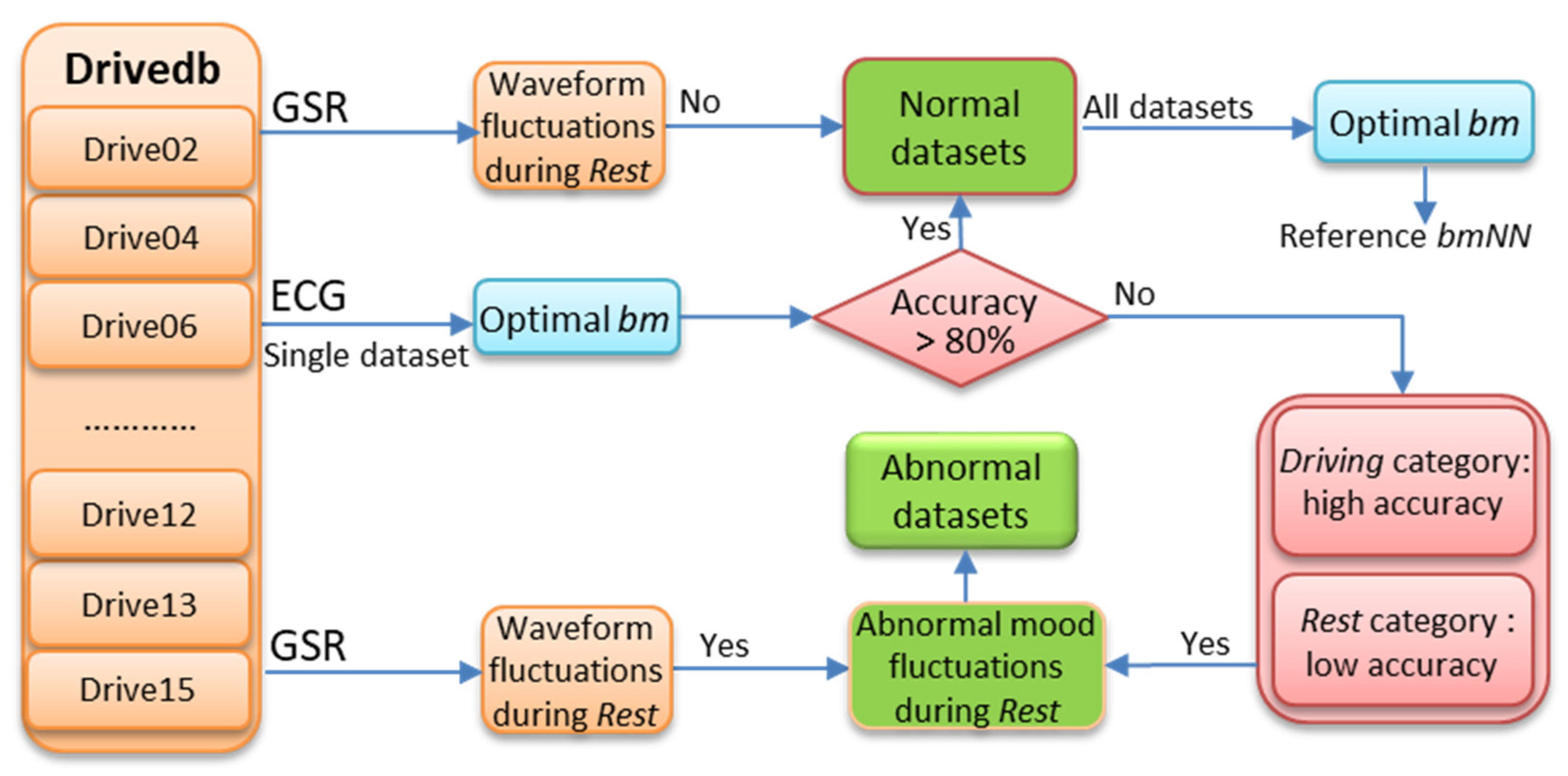
Although there were no detailed records of the data about unexpected events, inferences were made based on the changes in GSR signals and classification results. If the difference in stress levels between rest and driving states was clearly distinct, it was possible to obtain high classification accuracy (>80%). However, if abnormal events caused emotional changes during the rest period, the classification accuracy was likely compromised (<80%). For the datasets with identification accuracy lower than 80%, the classification accuracies for the driving and rest categories were recorded separately to determine that the low total accuracy was caused by the rest category. Simultaneously, GSR signal waveform changes during Rest were observed, and the reasons for the changes in classification accuracy were analyzed. Combined with the classification accuracy and waveform changes of the GSR in the rest period, the datasets with abnormal mood fluctuations were determined. The classification results of the abnormal datasets were not counted. Thus, we eliminated the impact of abnormal datasets in the driving stress database to improve the overall accuracy of the stress assessment. Figure 2 shows a block diagram of the recognition strategy for driving stress of the datasets in the drivedb database.

2.2. ECG Signal Preprocessing

The ECG signals were processed using the QRS detector based on the Pan–Tompkins algorithm [24]. The interbeat (RR) interval sequence was obtained from the ECG signals of each driving section to extract the NNI value.

2.3. Sample Length Selection

To extract the characteristic value of the beating mode, an appropriate sample length (L) was selected. In a previous study [19], HRV analysis was performed using time intervals of 300 s. In this study, 200 NNIs (L = 200, approximately 2–3 min) were chosen as fixed sample lengths, and 10 NNIs were advanced each time to generate a new sample. Table 1 shows the corresponding sample sizes for the different driving sections.

2.4. Feature Extraction with bmNN

In this study, the NNI output of the ECG signals was mapped to a binary sequence using statistical tools for linguistics to simplify the dynamics. As shown in Figure 3, an NNI time series with length L = 200 can be written as {NNI1,NNI2,…,NNIL}, where NNIn is the interval after the nth heartbeat. The NNI of each pair of consecutive heartbeats was assigned a subscript of zero or one according to the decrease or increase in the NNI.
I n = { 0 ,   if   N N I n N N I n 1 , 1 ,   if   N N I n > N N I n 1 .
A total of m + 1 consecutive NNIs were mapped to a binary sequence of length m, an m-bit word. Each m-bit word represents a unique fluctuation pattern within that time. After moving one data point at a time, the algorithm generated a set of m-bit words throughout the time series that reflected the underlying dynamics of the original time series. Different dynamics produce different distributions of these m-bit words. Each m-bit word represents a heartbeat mode and was marked with the symbol, bm. For an m-bit word, the range of values that bm (total 2m bms) could take was from 0 to 2m − 1. As shown in Figure 3, when m = 4, the 4-bit word “0011” corresponded to bm = 3 (2 + 1), whereas the 4-bit word “0110” corresponded to bm = 6 (4 + 2). In an NNI time series with length L, after the value of m was determined, the times of occurrence for the different bms in that period were counted to calculate the frequency of bm (denoted by bmNN).
b m N N = ( the   times   of   occurrence   for   the   b m ) / ( L m + 1 ) .
In this study, we chose L to be 200 and m to be 4; then, each sample with L = 200 could statistically generate 16 (24) bms, corresponding to 16 values for bmNN. Additionally, the average value of all NNIs (avNN, unit: s) in each sample was calculated.
Using the value of bmNN as the feature, the relationship between different bms and mental states was further analyzed using the k-NN classification algorithm.

2.5. Classification

2.5.1. Classifier for Classification

The objective of this study was to analyze the correlation between heartbeat mode and stress in the public driving stress database. For different samples in the driving dataset, the bmNN values corresponding to the same stress should be closer. The classification rules of the k-NN algorithm are based on the idea that data points of the same type will be closer in the feature space [25]. Since the data for each driving dataset were limited, and to intuitively explain the relationship between bmNN and stress, we chose the k-NN classification algorithm. Here, the Euclidean distance and a k value equal to five were used for the calculation.

2.5.2. Heartbeat Mode Analysis

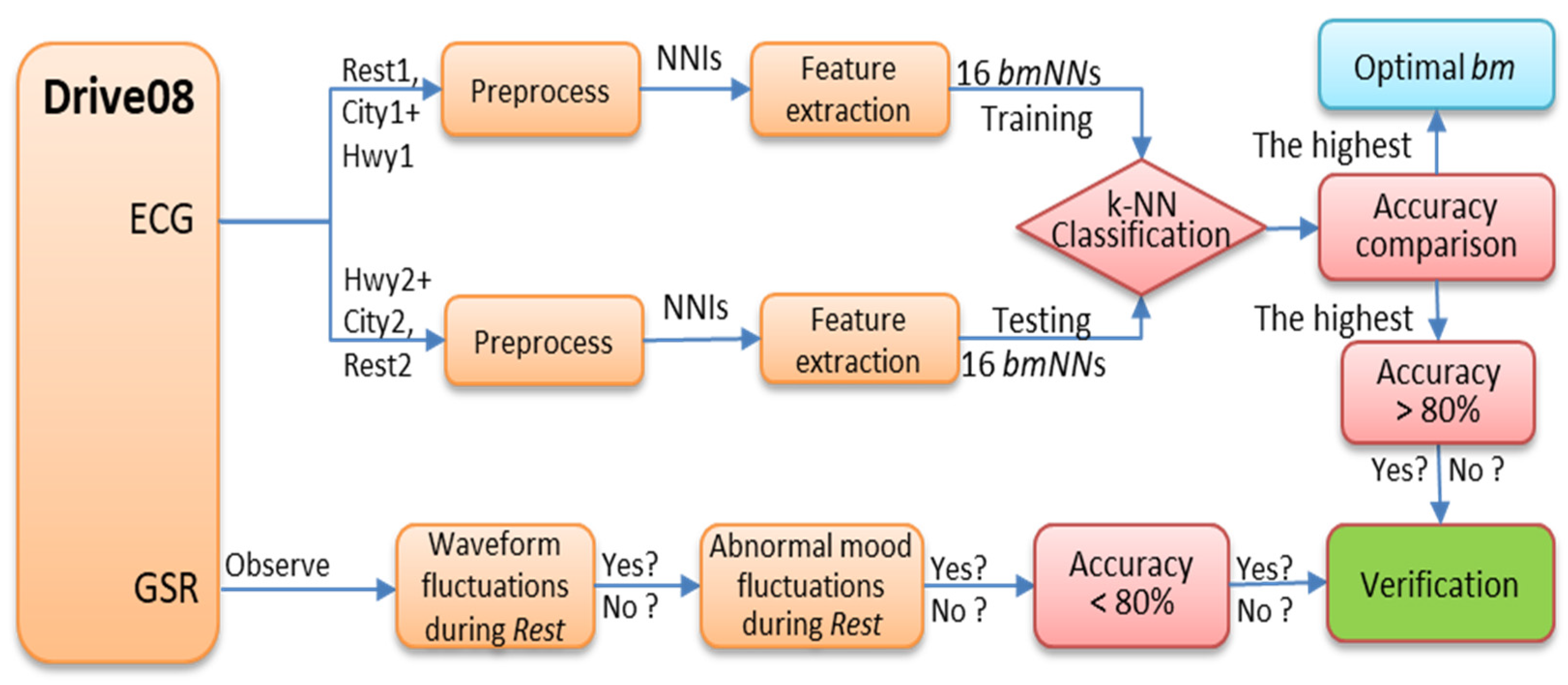
To verify the changes in bm in different driving sections, the test dataset was not selected from the same driving section as the training dataset. All samples were used for either training or testing without deleting any data, to analyze the stress state of the entire driving process as completely as possible. For the six driving sections, Rest1, City1, and Hwy1 were used as the training set, and Rest2, Hwy2, and City2 were used as the test set. The corresponding stress labels were “0,” “1,” and “2.” Label “0” represents low stress for Rest, “1” represents medium stress for Hwy, and “2” represents high stress for City.
In this study, only one feature of the ECG signals (i.e., bmNN) and the simplest k-NN classification algorithm were used to train the network with data from the first half of the driving sections of each driving dataset. The network was then used to identify and classify the stress levels of the second half of the driving sections of the corresponding dataset. We mainly analyzed the results of the two stress categories (rest/driving) to determine the optimal bm most related to driving stress. Figure 4 shows a block diagram of the heartbeat mode-based stress detection for Drive08 in the drivedb database.

2.5.3. Classification Steps

The following steps were carried out for classification:
  • The single driving data of the 10 driving datasets were first classified on two stress levels: rest or driving (0\1 + 2). All 16 values for bm were traversed, and the bm with the highest classification accuracy was recorded as the optimal bm for this round of driving classification.
  • For the data with classification accuracy higher than 80% among the 10 driving tests, classification was carried out after merging all datasets. Similarly, all 16 values of bm were traversed, and the bm with the highest classification accuracy was recorded and taken as the reference bm value for all classification tasks. For each round of classification, three different feature values were calculated (i.e., avNN, reference bmNN, and optimal bmNN).
  • For data with classification accuracy lower than 80% among the 10 driving tests in Step 1, the classification accuracies for the 0 and 1 + 2 categories were recorded alongside the total accuracy of each driving dataset. Simultaneously, GSR signal waveform fluctuations during Rest were observed, and the reasons for the changes in classification accuracy were analyzed.

3. Results

3.1. Classification Results of Driving Datasets with Accuracy above 80%

We identified 10 single driving datasets and classified them based on two stress levels. Six driving datasets (Drive02\04\06\08\11\13) had a classification accuracy of more than 80% for the optimal bmNN feature value. Table 2 shows the classification results of these six driving datasets using different feature values. The samples in these six driving datasets were merged based on the different driving sections and classified into two categories, with a corresponding optimal bm value of 12. The “Total” column in Table 2 shows the classification results. When bm equaled 12, the corresponding reference bmNN feature value was used to classify all six driving datasets. We represented the results of the reference bmNN feature in the second row under the 0\1 + 2 category and 0\1\2 category, whereas the first row shows the classification results of the avNN feature; the third row shows the classification results when the optimal bm value was used. Table 3 shows the average values of avNN, reference bmNN, and optimal bmNN for the different driving sections of Drive02\04\06\08\11\13.

3.2. Classification Results of Driving Datasets with Accuracy below 80%

Among the 10 driving datasets, the classification accuracy obtained by four of them (Drive07\10\12\15) was less than 80% for the optimal bmNN feature. Table 4 summarizes the total accuracy of each driving dataset as well as the classification accuracy for the 0 and 1 + 2 categories.

3.3. Interpretation of Results

Based on the 0\1 + 2 classification method, when the six driving datasets (Drive02\04\06\08\11\13) used the optimal bmNN as the feature value, the average identification accuracy reached 93.7%, which was higher than the 76.1% identification accuracy achieved when avNN was used as the feature value. This indicates that the bmNN value was more closely related to driving stress than was the average heart rate, and selecting the bm value achieved the classification of driving stress. However, the classification results of Drive11\13 when avNN was used as the feature value were 100% accurate, which was higher than that achieved when using bmNN as the feature value. The superior performance of avNN as a feature value for Drive11\13 identification might be related to specific individuals. Further experiments are needed to discover whether the stress level changes according to avNN or bmNN and if there are certain rules regarding this change.
When bm equaled 12, the identification accuracy of Drive13 was only 55.2%; however, when bm equaled 15, the identification accuracy increased to 90.6%. Owing to this significant difference in identification accuracy, it was speculated that bm, which represents stress level, could vary across different driving experiments. For Drive13, the stress expression was closely related to “1111”.
Table 3 shows the average bmNN values during different driving sections of the six driving datasets (Drive02\04\06\08\11\13). It was necessary to focus on the changes in Drive04, because for the other five driving datasets, the average feature values of bmNN for the different driving sections followed the same order of Rest > Hwy > City. This was different for Drive04; when bm was 12, the average values of bmNN were Rest (0.117) > City (0.063) > Hwy (0.028); when bm was 4, the average values of bmNN were Hwy (0.127) > City (0.074) > Rest (0.031). For Drive04, although the different driving sections all showed significant changes in the average bmNN value, the trends were different when bm took the reference value of 12 compared to when bm took the optimal value of 4. The unexpected events during the driving process and the personality of the driver were the reasons that led to these changes.
Table 4 shows the identification results for the remaining four datasets (Drive07\10\12\15). With the optimal bm value, the corresponding bmNN feature identification accuracy was respectively 73.2, 57.9, 56.5, and 63.4%, whereas the identification accuracy for category 0 alone was respectively 48.6, 17.9, 15.6, and 30.8%. For category 1 + 2 alone, it was 98.6, 96.6, 91.9, and 100%. The k-NN classification algorithm resulted in almost perfect identification accuracy for category 1 + 2; however, its performance decreased for category 0. This might be because, during the rest periods for these four driving datasets, unexpected events occurred that led to intense emotional fluctuations.
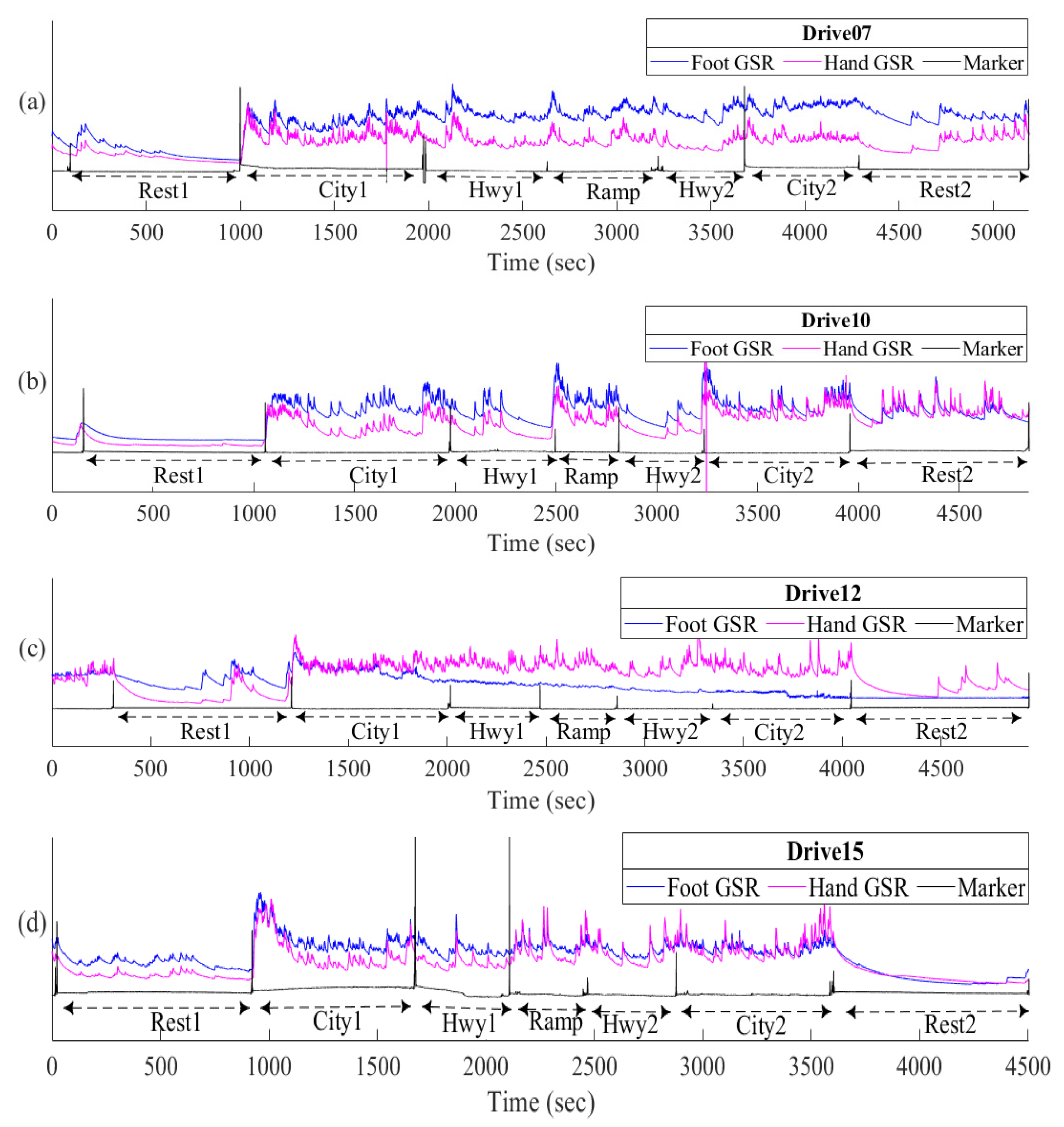
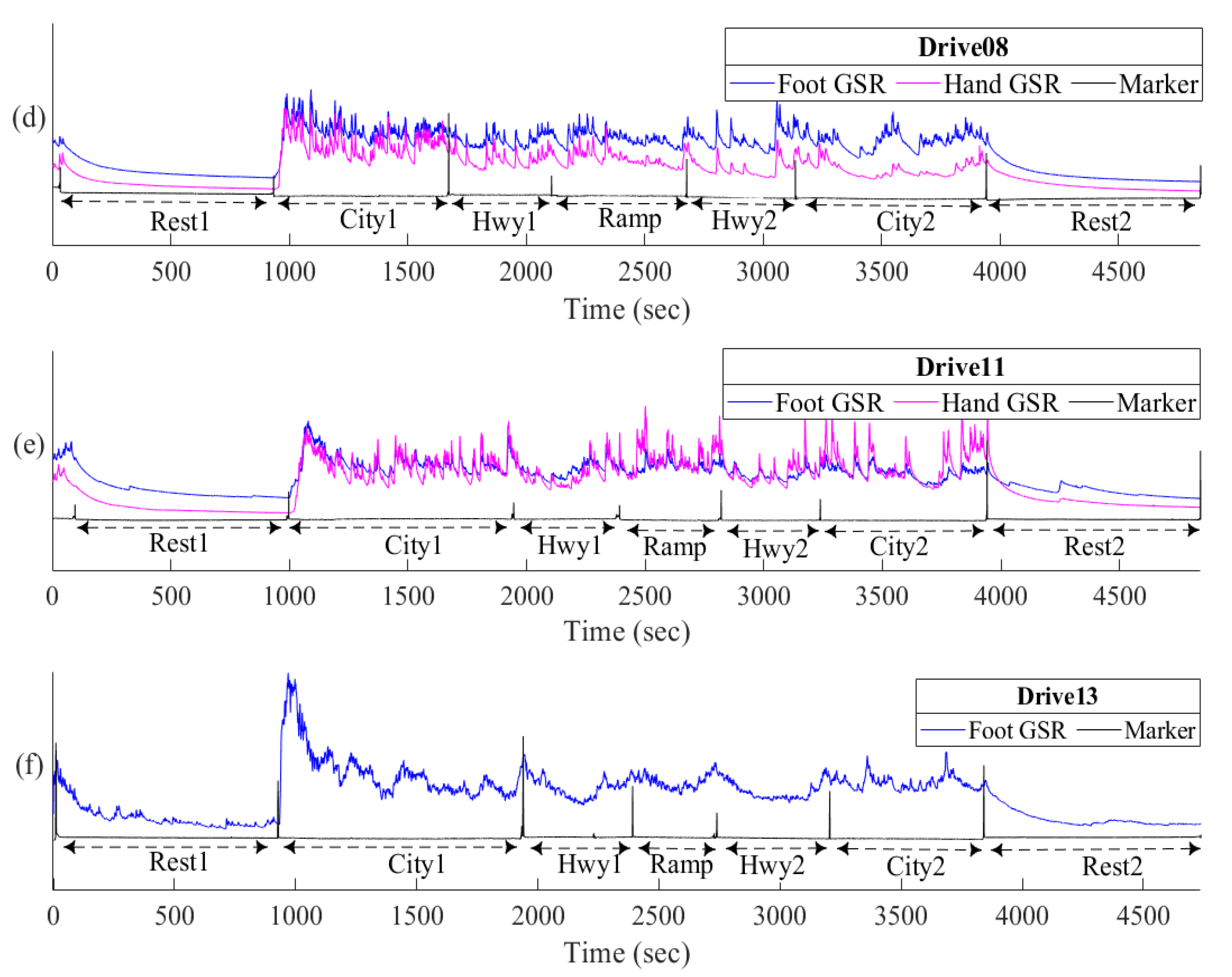
Subsequently, the GSR signals of all datasets during the rest period were compared to verify the above speculation. Figure 5 shows the GSR waveforms of the four driving datasets with an accuracy below 80%, whereas Figure 6 shows the GSR waveforms of the six driving datasets with an accuracy above 80%.
Figure 5a,b show that during Rest2 of Drive07\10, the GSR waveforms showed abnormal fluctuations. During Rest1 and Rest2 of Drive12, the GSR waveforms also showed abnormal fluctuations, which manifested in the foot GSR signals in Figure 5c. During Rest1 of Drive15, the GSR waveforms showed abnormal fluctuations, as well (see Figure 5d). As a result, the GSR waveforms during the rest periods of these four driving datasets showed abnormal fluctuations, which is consistent with the previous hypothesis, which posits that emotional fluctuations during rest periods cause low identification accuracy using the optimal bmNN feature.
From the six driving datasets having high identification accuracy (see Figure 6), it was observed that, apart from Drive04 (see Figure 6b), the other five driving datasets showed no fluctuations in the GSR waveforms during the rest periods. Since there was no additional information provided by the designers of the experiment, it was difficult to further analyze the abnormal performance of Drive04 during the rest periods. However, the fluctuations in the GSR waveforms indicated the occurrence of intense emotions, which might cause sudden changes in the bmNN value.

4. Discussion

In previous studies of stress detection based on the drivedb database, a common method was to take 5 min or less data of different driving sections as a sample, integrate all driving datasets for sample training with the help of a machine-learning method, and detect the stress on two (stress/no stress) or three (low, medium, and high) levels [19,21,23,25]. Through different classification algorithms and combinations of multiple features from different physiological signals, these previous studies achieved good classification results. However, those studies neglected the physiological differences of different individuals in driving stress; they were also incapable of analyzing the impact of abnormal events for stress detection in each driving process.
In this study, only one feature of the ECG signals (i.e., bmNN) and the simplest k-NN classification algorithm were used to train a network with data from the first half of the driving sections of each driving dataset. This was then used to identify and classify the stress levels of the second half of the driving sections of these driving datasets. This was unprecedented, given that most previous studies merged different driving datasets to classify stress levels on different driving sections. In addition, for different driving datasets, we chose different bm values for stress detection to conduct personalized analysis. Combined with the classification accuracy and waveform changes in the GSR during the rest period, the datasets with abnormal mood fluctuations were determined. The classification results of the abnormal datasets were not counted. Thus, we eliminated the impact of abnormal datasets in the driving stress database to improve the overall accuracy of the stress assessment. Table 5 shows comparisons of this and related works for stress detection using the drivedb database.
Based on the optimal bm value selected for each driving dataset, samples of every 200 NNIs (approximately 2–3 min) were classified based on stress. Using the 0\1 + 2 classification method, the average identification accuracy for the six driving datasets was 93.7%, whereas the average identification accuracy values for the remaining four driving datasets were low. However, the GSR waveforms of these four datasets exhibited abnormal fluctuations during the rest periods, which might explain the low identification accuracy. These 10 driving datasets revealed that the bmNN value had a high correlation with psychological stress, which was reflected in real time by changes in GSR signals.
In the study by Healey et al. [19], GSR had the best real-time correlation with stress, followed by heart rate and HRV frequency domain indicators. We also discovered that the different driving sections of Drive 02\04\06\08\11\13 had average avNN values in the order of Rest > Hwy > City. That is, stress was correlated with heart rate such that the latter increased with the former, which is consistent with existing research results [19,21]. However, the change in the average avNN value was not significant, and differences existed among individuals. For the six driving datasets classified with the avNN feature, the average classification accuracy was 76.1%, whereas the classification accuracy for Drive08 was only 26.8%. For Drive08, the average values of avNN were Rest (0.987) > Hwy (0.969) > City (0.914), presented in Table 3, and the similar values of avNN in the different driving sections were the reason for the extremely low classification accuracy. Meanwhile, the identification accuracy for Drive07\15 data classified into the 0 category was good, indicating that the avNN feature value did not exhibit any changes to the GSR signal during the rest periods.
After comparing it with the avNN feature value, the value of bmNN was correlated to the GSR signals, which reflected the emotional changes in real time. Additionally, owing to individual differences, the avNN values for some driving datasets did not change significantly when the stress changed. For bmNN, different values for m and bm were used to, through trial and error, find the relevant beating mode to the individual stress to achieve an individualized analysis. The average bmNN feature values for the three driving sections of the five driving datasets (Drive02\06\08\11\13) followed the order of Rest > Hwy > City. That is, the bm feature value decreased as the stress increased. This verifies the findings of McCraty et al. [16], indicating that negative emotions of stress negatively impact the coherence of heart-rhythm patterns.
In this study, classification was discussed using one feature. For some driving datasets, two features, avNN + bmNN or bmNN + bmNN, were used in combination to improve the classification accuracy. However, further verification through experiments is necessary to decide whether such results are meaningful, hence different combinations of features were not used for stress detection in this study.

5. Conclusions

McCraty et al. [16] mentioned that the synchronization between emotional and physiological dynamics is directly related to rhythmic patterns in the heart rate (the order of the rate of change over time), not the heart rate itself at any point in time. Furthermore, this study’s results demonstrated the existence of this HRV rhythm change in synchronization with emotions. After combining ML methods and heartbeat mode analysis, as well as choosing values for m and bm, we found that the HRV rhythms corresponded to driver stress. The different heartbeat modes in the time series were summarized, and specific heart-rhythm patterns related to different driving stresses were obtained. It was also concluded that the heartbeat mode was correlated with the GSR signal, reflecting real-time abnormal mood fluctuations.
The proposed method based on heartbeat mode can reveal the variation rule of heart-rate variability on a shorter time scale (m + 1 NNIs; in this study, m = 4), which is less affected by the abnormal value of NNI caused by false detection. The proposed bmNN feature is an effective index for evaluating the dynamic changes of ANS under stress. Thus, it would be feasible to conduct a personalized analysis to further study the interaction between physiology and psychology.
In future research, we aim to create a larger dataset for ECG emotional states to investigate the differences between individuals and emotions using ML methods and heartbeat mode analysis with m and bm values. An example is the feeling of “heartbeat” between people when they are in love, which might not be only a figurative metric; it might correspond to specific beating modes of the heart. Based on our findings, such phenomena can now be studied.

Author Contributions

Conceptualization, D.H. and L.G.; Data curation, D.H.; Formal analysis, D.H.; Funding acquisition, L.G.; Investigation, D.H.; Methodology, D.H.; Supervision, L.G.; Writing—original draft, D.H.; Writing—review and editing, D.H. All authors have read and agreed to the published version of the manuscript.

Funding

This work was supported by the HFIPS Director’s Fund, Grant No. YZJJ2021QN25. Key research projects supported by the National Natural Science Foundation of China, Grant No. 92067205. Major science and technology project of Anhui Province, Grant No. 202103a05020022.

Institutional Review Board Statement

Not applicable.

Informed Consent Statement

Not applicable.

Data Availability Statement

Not applicable.

Acknowledgments

This work was partly carried out at the Robotic Sensors and Human–Computer Interaction Laboratory, Hefei Institute of Intelligent Machinery, Chinese Academy of Sciences.

Conflicts of Interest

The authors declare no conflict of interest.

References

  1. Alshamrani, M. An Advanced Stress Detection Approach based on Processing Data from Wearable Wrist Devices. Int. J. Adv. Comput. Sci. Appl. 2021, 12, 399–405. [Google Scholar] [CrossRef]
  2. Iqbal, T.; Redon-Lurbe, P.; Simpkin, A.J.; Elahi, A.; Ganly, S.; Wijns, W.; Shahzad, A. A Sensitivity Analysis of Biophysiological Responses of Stress for Wearable Sensors in Connected Health. IEEE Access 2021, 9, 93567–93579. [Google Scholar] [CrossRef]
  3. Samson, C.; Koh, A. Stress Monitoring and Recent Advancements in Wearable Biosensors. Front. Bioeng. Biotechnol. 2020, 8, 1037. [Google Scholar] [CrossRef]
  4. Thayer, J.F.; Åhs, F.; Fredrikson, M.; Sollers, J.J.; Wager, T.D. A meta-analysis of heart rate variability and neuroimaging studies: Implications for heart rate variability as a marker of stress and health. Neurosci. Biobehav. Rev. 2012, 36, 747–756. [Google Scholar] [CrossRef]
  5. Elgendi, M.; Menon, C. Machine Learning Ranks ECG as an Optimal Wearable Biosignal for Assessing Driving Stress. IEEE Access 2020, 8, 34362–34374. [Google Scholar] [CrossRef]
  6. Dalmeida, K.M.; Masala, G.L. Hrv features as viable physiological markers for stress detection using wearable devices. Sensors 2021, 21, 2873. [Google Scholar] [CrossRef]
  7. Shaffer, F.; Ginsberg, J.P. An Overview of Heart Rate Variability Metrics and Norms. Front. Public Health 2017, 5, 258. [Google Scholar] [CrossRef] [Green Version]
  8. Kim, H.G.; Cheon, E.J.; Bai, D.S.; Lee, Y.H.; Koo, B.H. Stress and heart rate variability: A meta-analysis and review of the literature. Psychiat. Investig. 2018, 15, 235–245. [Google Scholar] [CrossRef] [Green Version]
  9. Kumar, M.; Zhang, W.; Weippert, M.; Freudenthaler, B. An Explainable Fuzzy Theoretic Nonparametric Deep Model for Stress Assessment Using Heartbeat Intervals Analysis. IEEE Trans. Fuzzy Syst. 2020, 29, 3873–3886. [Google Scholar] [CrossRef]
  10. Burma, J.S.; Graver, S.; Miutz, L.N.; Macaulay, A.; Copeland, P.V.; Smirl, J.D. The validity and reliability of ultra-short-term heart rate variability parameters and the influence of physiological covariates. J. Appl. Physiol. 2021, 130, 1848–1867. [Google Scholar] [CrossRef]
  11. Zhao, L.; Li, P.; Li, J.; Liu, C. Influence of ectopic beats on heart rate variability analysis. Entropy 2021, 23, 648. [Google Scholar] [CrossRef] [PubMed]
  12. Lombardi, F.; Huikuri, H.; Schmidt, G.; Malik, M. Short-term heart rate variability: Easy to measure, difficult to interpret. Heart Rhythm 2018, 15, 1559–1560. [Google Scholar] [CrossRef] [PubMed] [Green Version]
  13. Shaffer, F.; Meehan, Z.M.; Zerr, C.L. A critical review of ultra-short-term heart rate variability norms research. Front. Neurosci. 2020, 14, 594880. [Google Scholar] [CrossRef] [PubMed]
  14. Roman-Juan, J.; Bornas, X.; Zuzama, N.; Fiol-Veny, A.; Balle, M. Decrements in Adolescent Cardiac Complexity During Mother-Adolescent Conflicts. Appl. Psychophysiol. Biofeedback 2021, 46, 259–270. [Google Scholar] [CrossRef]
  15. Kimmel, M.C.; Fransson, E.; Cunningham, J.L.; Brann, E.; Grewen, K.; Boschiero, D.; Chrousos, G.P.; Meltzer-Brody, S.; Skalkidou, A. Heart rate variability in late pregnancy: Exploration of distinctive patterns in relation to maternal mental health. Transl. Psychiat. 2021, 11, 286. [Google Scholar] [CrossRef]
  16. McCraty, R.; Zayas, M.A. Cardiac coherence, self-regulation, autonomic stability and psychosocial well-being. Front. Psychol. 2014, 5, 1090. [Google Scholar] [CrossRef] [Green Version]
  17. Pereira, T.; Almeida, P.R.; Cunha, J.P.S.; Aguiar, A. Heart rate variability metrics for fine-grained stress level assessment. Comput. Meth. Prog. Biomed. 2017, 148, 71–80. [Google Scholar] [CrossRef]
  18. Gedam, S.; Paul, S. A Review on Mental Stress Detection Using Wearable Sensors and Machine Learning Techniques. IEEE Access 2021, 9, 84045–84066. [Google Scholar] [CrossRef]
  19. Healey, J.A.; Picard, R.W. Detecting stress during real-world driving tasks using physiological sensors. IEEE Trans. Intell. Transp. Syst. 2005, 6, 156–166. [Google Scholar] [CrossRef] [Green Version]
  20. Goldberger, A.L.; Amaral, L.A.; Glass, L.; Hausdorff, J.M.; Ivanov, P.C.; Mark, R.G.; Mietus, J.E.; Moody, G.B.; Peng, C.K.; Stanley, H.E. PhysioBank, PhysioToolkit, and PhysioNet: Components of a new research resource for complex physiologic signals. Circulation 2000, 101, e215–e220. [Google Scholar] [CrossRef] [Green Version]
  21. Chen, L.; Zhao, Y.; Ye, P.; Zhang, J.; Zou, J.Z. Detecting driving stress in physiological signals based on multimodal feature analysis and kernel classifiers. Expert Syst. Appl. 2017, 85, 279–291. [Google Scholar] [CrossRef]
  22. Aristizabal, S.; Byun, K.; Wood, N.; Mullan, A.F.; Porter, P.M.; Campanella, C.; Jamrozik, A.; Nenadic, I.Z.; Bauer, B.A. The Feasibility of Wearable and Self-Report Stress Detection Measures in a Semi-Controlled Lab Environment. IEEE Access 2021, 9, 102053–102068. [Google Scholar] [CrossRef]
  23. Liu, Y.; Du, S. Psychological stress level detection based on electrodermal activity. Behav. Brain Res. 2018, 341, 50–53. [Google Scholar] [CrossRef] [PubMed]
  24. Pan, J.; Tompkins, W.J. A Real-Time QRS Detection Algorithm. IEEE Trans. Biomed. Eng. 1985, 32, 230–236. [Google Scholar] [CrossRef] [PubMed]
  25. Wang, J.S.; Lin, C.W.; Yang, Y.T.C. A k-nearest-neighbor classifier with heart rate variability feature-based transformation algorithm for driving stress recognition. Neurocomputing 2013, 116, 136–143. [Google Scholar] [CrossRef]
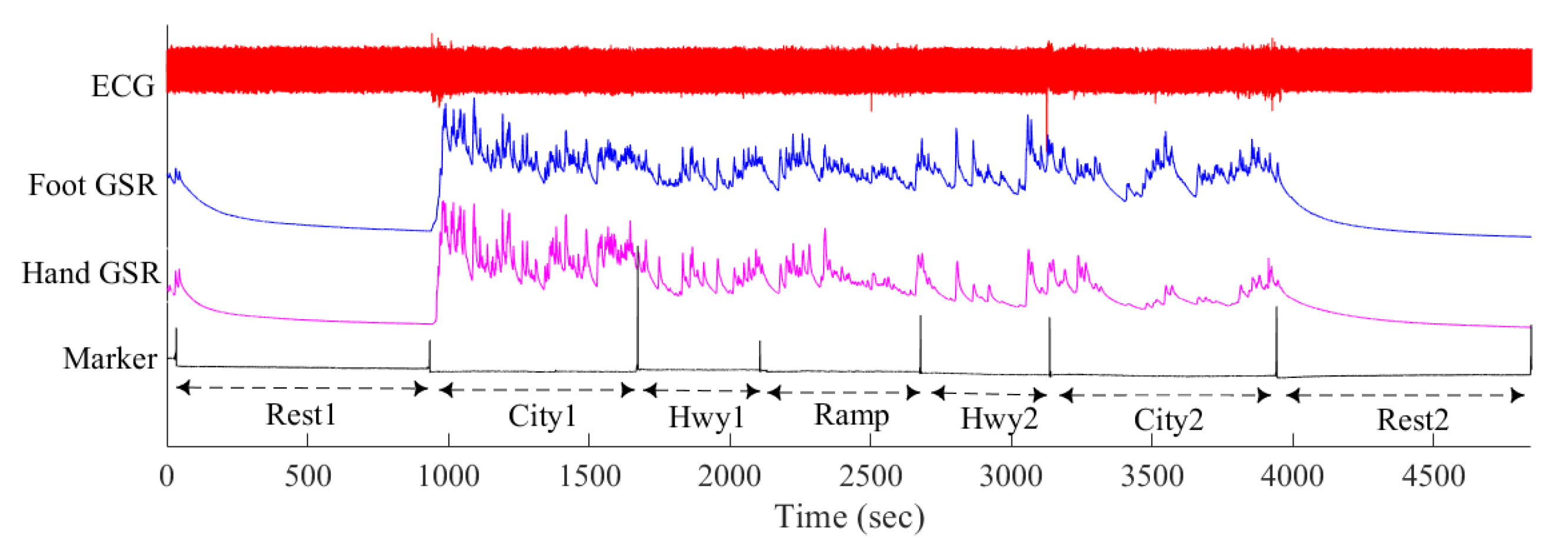
Figure 1. ECG, GSR, and marker signals of Drive08 in the drivedb database.
Applsci 12 01409 g001
Figure 2. Block diagram of the recognition strategy for driving stress of the datasets in the drivedb database.
Applsci 12 01409 g002
Figure 3. Schematic diagram of the mapping process from the ECG signal to a 4-bit word.
Applsci 12 01409 g003
Figure 4. Block diagram of the heartbeat mode-based stress detection for Drive08 in the drivedb database.
Applsci 12 01409 g004
Figure 5. GSR signals and marker signals of the six driving sections of Drive07\10\12\15: (a) GSR and marker signals of Drive07; (b) GSR and marker signals of Drive10; (c) GSR and marker signals of Drive12; (d) GSR and marker signals of Drive15. The foot GSR signal of Drive12 was inconsistent with the hand GSR signal, and the study referred to the hand GSR signal.
Applsci 12 01409 g005
Figure 6. GSR signals and marker signals of the six driving sections of Drive02\04\06\08\11\13: (a) GSR and marker signals of Drive02; (b) GSR and marker signals of Drive04; (c) GSR and marker signals of Drive06; (d) GSR and marker signals of Drive08; (e) GSR and marker signals of Drive11; (f) GSR and marker signals of Drive13. Drive02 and Drive13 lacked hand GSR signals and only had foot GSR signals. The foot GSR signal of Drive06 was inconsistent with the hand GSR signal, and the study referred to the foot GSR signal.
Applsci 12 01409 g006aApplsci 12 01409 g006b
Table 1. Time and sample size after segmentation of the 10 driving datasets.
Rec. NameSample Size/Time (s)Total Rec. Time (s)
Rest1City1Hwy1Hwy2City2Rest2
Drive0277/90060/70024/40014/30072/80068/8005000
Drive0481/90095/90030/4005/20039/50051/7004800
Drive06102/900108/74038/39029/35089/71092/8704780
Drive0789/90084/80054/60028/40042/50072/8005100
Drive0864/80049/60022/40021/40053/70064/11004840
Drive1074/80074/70041/48026/36061/60084/8004800
Drive1166/87070/83019/37018/35045/60054/8004800
Drive1256/80054/76022/40026/43048/62064/8004900
Drive1390/800135/90043/37041/38071/55091/8004700
Drive1569/87051/66016/34011/30047/60065/8504500
Table 2. Classification results of Drive02\04\06\08\11\13 as two or three categories.
ClassesFeaturesAccuracy (%)
MeanDrive02Drive04Drive06Drive08Drive11Drive13Total
0\1 + 2avNN76.170.168.491.026.810010070.9
bmNN/bm = 1287.092.998.992.910082.155.277.1
optimal bmNN93.792.910094.810083.890.677.1
0\1\2avNN59.150.663.261.013.879.586.257.9
bmNN/bm = 1269.177.394.768.696.459.018.750.4
optimal bmNN81.777.395.868.696.473.578.852.9
Table 3. Average values of avNN and bmNN for different driving sections of Drive02\04\06\08\11\13.
Rec. NameFeaturesAverage Feature Values
012
MeanRest1Rest2MeanHwy1Hwy2MeanCity1City2
Drive02avNN0.9040.9150.8930.8780.8880.8670.8500.8430.856
bmNN/120.1470.1350.1580.1170.1070.1270.0890.0760.101
Drive04avNN0.9180.8700.9670.8030.7880.8180.8060.7720.839
bmNN/120.1170.0960.1380.0280.0220.0350.0630.0630.063
bmNN/40.0310.0400.0210.1270.1450.1100.0740.0790.068
Drive06avNN0.7490.7340.7640.7010.6890.7120.6170.5850.649
bmNN/120.1050.0970.1130.0650.0740.0550.0710.0740.067
bmNN/90.0960.0860.1060.0620.0620.0620.0570.0500.063
Drive08avNN0.9870.9511.0230.9690.9530.9850.9140.8800.947
bmNN/120.1690.1580.1810.1270.1310.1240.0940.1020.086
Drive11avNN1.0110.9951.0270.9180.9110.9240.8990.8960.901
bmNN/120.1220.1270.1170.0520.0620.0420.0670.0750.059
Drive13avNN0.7200.7230.7170.6150.6030.6260.5840.5770.591
bmNN/120.0840.0830.0840.0780.0780.0770.0620.0770.047
bmNN/150.1760.1790.1730.0940.0780.1100.0570.0550.058
Notes: avNN, unit: s.
Table 4. Classification results of Drive07\10\12\15.
ClassesFeaturesAccuracy (%)
Drive07Drive10Drive12Drive15
Total01 + 2Total01 + 2Total01 + 2Total01 + 2
0\1 + 2avNN63.490.335.750.9010053.6010088.684.693.1
bmNN/bm=1265.531.910048.0094.353.6010063.430.8100
optimal bmNN73.248.698.657.917.996.656.515.691.963.430.8100
Table 5. Comparison of this and related works for stress detection using the drivedb database.
ReferenceSignalsFeaturesTechniques UsedDatasets
Required
for Training
Accuracy
(%)
Rest\Hwy\City
This workECGSingle
features:
bmNN Vs. avNN
Heartbeat mode analysis and k-NNSingle
driving
dataset
bmNN:
2 classes: 93.7%
3 classes: 81.7%
avNN:
2 classes: 76.1%
3 classes: 59.1%
Dalmeida et al.,
2021 [6]
ECGMultiple features:
avNN,
RMSSD,
TP, ULF,
SDNN
SVM, MLP, RF, and GBAll driving datasets2 classes
(Recall)
SVM: 79%
MLP: 81%
RF: 81%
GB: 80%
Elgendi et al.,
2020 [5]
ECG, EMG, GSR, RESPMultiple features:
automatic Selection
IPCA, CBC, KMC, and the k-NN-Weighted classifierAll driving datasets3 classes
ECG: 75.02%
GSR: 72.05%
Yun Liu et al.,
2018 [23]
GSRMultiple features:
18 features
Fisher projection and LDA All driving datasets3 classes: 81.8%
Lan-lan Chen et al., 2017 [21]ECG, EMG, GSR, RESPMultiple features:
73 features
SBL, PCA, SVM, and ELMAll driving datasets3 classes: 99%
Jeen-Shing Wang et al., 2013 [25] ECGMultiple features:
56 features
KBCS, PCA, LDA, and k-NN All driving datasets2 classes: 97.8%
Healey et al.,
2005 [19]
ECG, EMG, GSR, RESPMultiple features:
22 features
Fisher projection matrix and a linear discriminantAll driving datasets3 classes: 97.4%
Notes: connectivity-based clustering (CBC); extreme learning machine (ELM); gradient boosting (GB); interaction principal component analysis (IPCA); kernel-based class separability (KBCS); k-means clustering (KMC); k-nearest neighbor (k-NN); linear discriminant analysis (LDA); multilayer perceptron (MLP); principal component analysis (PCA); random forest (RF); support vector machine (SVM); sparse Bayesian learning (SBL).
Publisher’s Note: MDPI stays neutral with regard to jurisdictional claims in published maps and institutional affiliations.