Abstract
We propose and evaluate a procedure for the explainability of a breast density deep learning based classifier. A total of 1662 mammography exams labeled according to the BI-RADS categories of breast density was used. We built a residual Convolutional Neural Network, trained it and studied the responses of the model to input changes, such as different distributions of class labels in training and test sets and suitable image pre-processing. The aim was to identify the steps of the analysis with a relevant impact on the classifier performance and on the model explainability. We used the grad-CAM algorithm for CNN to produce saliency maps and computed the Spearman’s rank correlation between input images and saliency maps as a measure of explanation accuracy. We found that pre-processing is critical not only for accuracy, precision and recall of a model but also to have a reasonable explanation of the model itself. Our CNN reaches good performances compared to the state-of-art and it considers the dense pattern to make the classification. Saliency maps strongly correlate with the dense pattern. This work is a starting point towards the implementation of a standard framework to evaluate both CNN performances and the explainability of their predictions in medical image classification problems.
1. Introduction
Breast cancer is the most frequently diagnosed cancer among women worldwide and it is the second leading cause of death [1]. It has been shown that one woman in eight is going to develop breast cancer in her life and early diagnosis is one of the most powerful instruments we have in fighting the disease [2]. Full Field Digital Mammography (FFDM) is a non-invasive highly sensitive method for early stage breast cancer detection and diagnosis, and represents the reference imaging technique to explore the breast in a complete way [3,4]. One of the major issues in cancer detection is due to the presence of breast dense tissue. Breast density is defined as the amount of fibroglandular parenchyma or dense tissue with respect to the fat one as seen on a mammographic exam [5]. Since X-ray absorption coefficient for dense and cancerous tissues are similar, a mammogram with a very high percentage of fibroglandular tissue is less readable. In order to have a sufficient sensitivity in denser breasts, a higher radiation dose has to be delivered to the patient [6]. Moreover, breast density is an intrinsic risk factor in developing the disease [7,8,9]. For these reasons, a density standard has been established by the American College of Radiology (ACR) in 2013 [5] and it is reported on the Breast Imaging Reporting and Data System (BI-RADS) Atlas. The standard defines four qualitative classes: almost entirely fatty (A), scattered areas of fibroglandular density (B), heterogeneously dense (C) and extremely dense (D). Since mammographic density assessment made by radiologists suffers from a non-negligible intra and inter-observer variability [10], some automatic methods have been developed in order to make the classification reproducible. Many approaches use a two-step classification [11,12,13,14]: first, either they extract features from the images or apply a segmentation method and, afterwards, they train a classifier with a Support Vector Machine or other machine learning methods. In [15], a fully automated algorithm has been developed: the breast is segmented, density features are extracted and used to train and evaluate SVM classifiers with an accuracy of 84.47% on the miniMIAS dataset. In [16], Petroudi et al. conceived a method based on the statistical distribution of rotationally invariant filter responses in a low dimensional space, following the Third Edition of the BI-RADS standard (1998). In the last few years, deep learning-based methods have been developed with success in a wide range of medical image analysis problems [17]. The main advantage of deep learning-based classifier stands in their capability of analyzing data from different sources and automatically extracting image related features. Since features represent image properties that cannot be analytically described, they are not easily intelligible. Moreover, it is not straightforward to explain how such algorithms perform the classification. The detailed study of deep learning applications to medical images and their explainability is a challenge that can help medical physicists on tasks such as the data quality control and validation [18]. Explaining a deep learning based classifier is crucial in order to understand whether the classification is correct. In fact, since Convolutional Neural Networks are trained directly on images, it may happen that they focus their attention on uncorrelated or wrong parts of the images [19], introducing a bias in the classification. Moreover, there exists no standard to quantify when an algorithm is well explained or not. For this reason, we propose the Spearman’s rank correlation coefficient in order to verify at least the monotonic dependence between the pixel and the activation maps intensity. The lack of huge public labeled mammographic dataset is a major issue when dealing with deep machine learning models applied to mammography, because it implies the impossibility of comparing models using the same data [18]. As an example, one of the most used public analogic datasets of mammograms, called miniMIAS [20], is labeled by three qualitative classes that are Fatty (F), Fatty-Glandular (G) and Dense-Glandular (D), which are now obsolete. In this work, we trained a residual Convolutional Neural Network (CNN) [21] classifier and applied a widely used explanation method to assess which are the main factors affecting the classifier performance not only in terms of accuracy but also in terms of a posteriori explanation and, consequently, interpretation of the AI model. The classifier has been trained to classify breast density according to the fifth edition of the BI-RADS standard. We considered both the figures of merit and the saliency maps produced by the grad-CAM algorithm, then interpreted the goodness of our model by computing the Spearman’s rank correlation between the input images and their saliency maps. This method has never been used on natural images that are three-channel images; on the contrary, a mammogram can be interpreted as a result of a pre-processed signal. The classification performances have been studied considering different proportions of density class labels in the train and test datasets and different pre-processing pipelines.
2. Materials and Methods
2.1. Data
Due to the lack of public research databases populated with digital mammograms to use in AI applications devoted to density class identification [20,22], we analyzed Full-Field Digital Mammograms (FFDM) collected within the RADIOMA project and described in [23]. This private repository includes data from 1662 subjects (6648 images) acquired at the University Hospital of Pisa (Azienda Ospedaliera Universitaria Pisana AOUP, Pisa, Italy). Informed consent was obtained from all the participants included in the present study. The team, which included Physicists, Radiologists and a Radiology Technician, that worked at the data collection has implemented and applied the following inclusion criteria to select images from the wider clinical database available:
- All exam reports were required to be negative. Whenever possible, a later mammographic exam in medical records has been examined to verify the current state of health of women.
- Badly exposed X-ray mammograms were not collected.
- Only exams including all the four projections usually acquired in mammography (cranio-caudal—CC—and medio-lateral oblique—MLO—of left and right breast) were chosen.
The exams were acquired with the GE Senograph DS imaging systems available at the University Hospital. For each exam, data annotation, which is the assessment of density class, has been performed by a Radiologist with specific expertise in mammography, who relied on the medical report already available within the routine clinical evaluation. The distribution of the 1662 exams over the 4 density classes is reported in Table 1, where the average age is reported for each class.

Table 1.
Dataset population and age distribution (described in terms of the mean, standard deviation and median values) of the exams over the four BI-RADS density classes (A, B, C, D).
2.2. Methods
Fully understanding a CNN behavior is a non-trivial problem and there are currently no protocols or guidelines establishing a strict and robust validation method. Furthermore, most datasets used in published works are not accessible and, hence, comparisons among different methods and algorithms are hampered. Lastly, two of the most used data sets, miniMIAS [20] or the CBIS-DDSM [22] contain only digitized analog mammograms. Using different datasets in a reproducibility test does not guarantee the achievement of the same results. To further test the consistency of AI-based results, it is advisable to investigate which characteristics of the images, of the acquisition protocols and of the manipulation pipelines sensibly affect the performances of deep learning algorithms. Studying the roboustness of algorithms is important in order to understand the boundaries in which the classifier can be applied. Since the data set of this study has been collected from a clinical database, it is crucial to study whether and under which conditions it may be applied on a screening population. To this purpose, we trained from scratch a residual CNN to classify breast density in four categories, according to the Fifth Edition of BI-RADS standard, and systematically evaluated the impact on the CNN performance of:
- The different proportion of mammograms belonging to the four density categories in the training and test sets;
- Either including or not an image pre-processing step.
The effect of the latter on the model interpretability is also studied and discussed. Finally, a simple metric to quantify the appropriateness of the chosen explainability framework is proposed. The choice of a CNN to perform the classification was due to the change of the BI-RADS classes definition from the 4th Atlas to the 5th one. In fact in the last edition, the definition through the quantification criteria based on the percentage of dense and fat tissue has been abandoned and the classes were defined through image examples and textual description. In order to capture this new definition, the deep learning based methods seem to be the most appropriate.
2.2.1. Data Preparation and Pre-Processing
Mammograms have been extracted from the DICOM files using DICOM-ToolKit, since they were stored in a jpeg lossless compression format. The CNN training procedure with Keras requires 8-bit images; therefore, we had to convert the 12-bit mammograms into this format. By visually inspecting the dataset, we found out that the images acquired have some burnt pixels that always assume the maximum grayscale value, while most of the signal is in another part of the histogram. Furthermore, having the dataset been extracted from a clinical sample instead of a screening one, we found clips, that are used after a biopsy, represented in many images. These clips appear whiter than the expected maximum breast signal intensity. As we could not normalize the mammograms to the maximum intensity values, we set a maximum threshold to 3500 for the pixel value, then we linearly scaled the image pixel values between the minimum intensity and the maximum of 3500; finally the values have been converted to 8 bits and the exams have been stored in the Portable Network Graphics (PNG) format. All the PNG images have been inspected one by one in order to eliminate some problematic images which were not correctly acquired.
2.2.2. Standard Image Pre-Processing Step
The GE Senograph mammograms are 1914 × 2294 pixel images, where the breast representation often occupies about half of the image width. To limit the data processing time (i.e., to minimize the number of input nodes of the CNN and thus the weights to be learned during the training process) we decided to crop the images according to the minimum bounding box enclosing the breast view. To this purpose, we attempted to recognize the skin line of the breast using a marching-square algorithm for 2D images [24,25], available within the scikit-learn Python package [26]. To properly identify the breast margin, we set the starting threshold at the intensity level of 50 while leaving the other parameters to default values; then we cropped the images to the minimum bounding box including the margin, as shown in Figure 1.
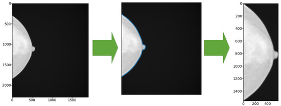
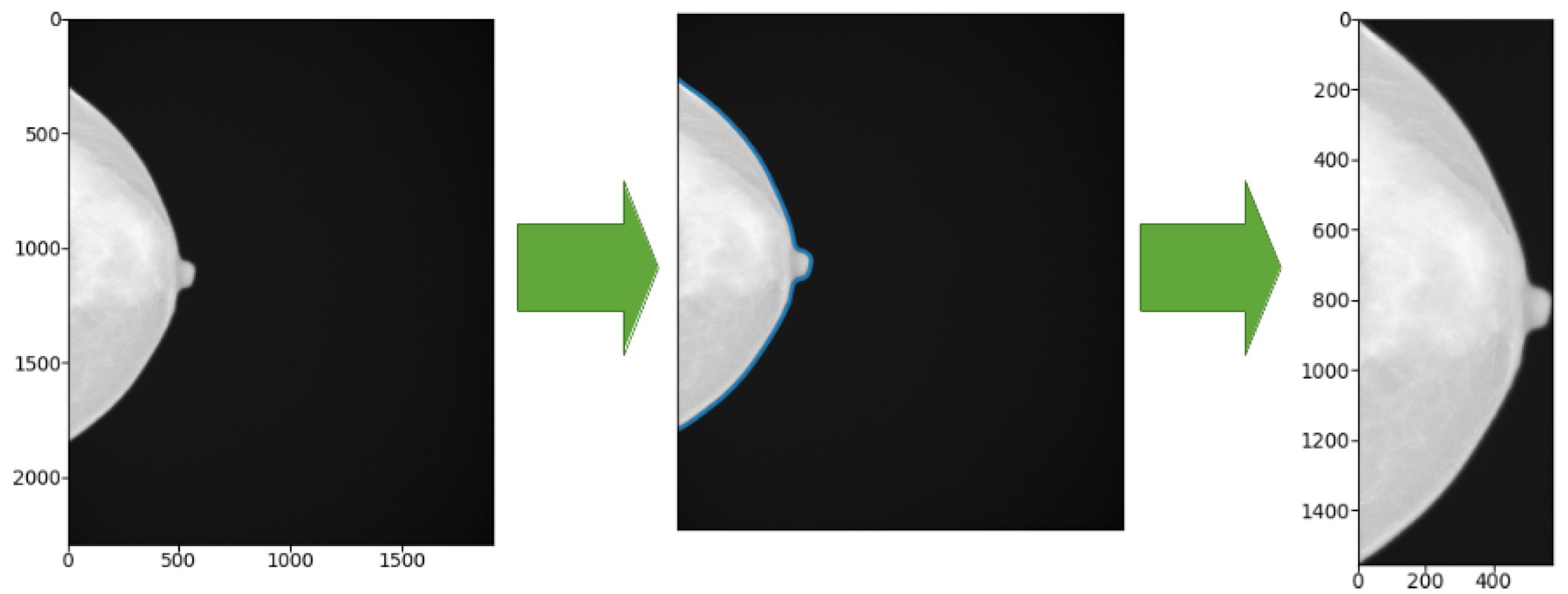
Figure 1.
Left: original image. Center: the blue line shows the contour identified by the marching-square algorithm. Right: cropped image according to the bounding box enclosing the breast view.
2.2.3. Additional Pre-Processing Step: Pectoral Muscle Removal
As an additional pre-processing step, we designed an algorithm to remove the pectoral muscle that appears on medio-lateral oblique projections. First, all the medio-lateral oblique projections have been oriented in the same way, i.e., left ones have been flipped horizontally. Then we chose a square which contains the pectoral muscle and cropped the image. A Gaussian filter has been applied to all the selected regions in order to reduce noise. For each image, the regions have been binarized with an adaptive threshold method based on inverted binary thresholding and Otsu’s binarization and the mask containing the pectoral muscle (white) and the rest of the breast (black) have been produced. The coordinates of the points at the edge of the pectoral muscle have been fitted with a linear function and the values of all the pixels above the edge have been replaced with the mean gray level of the breast. In Figure 2, we reported an example of these operations.
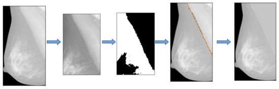
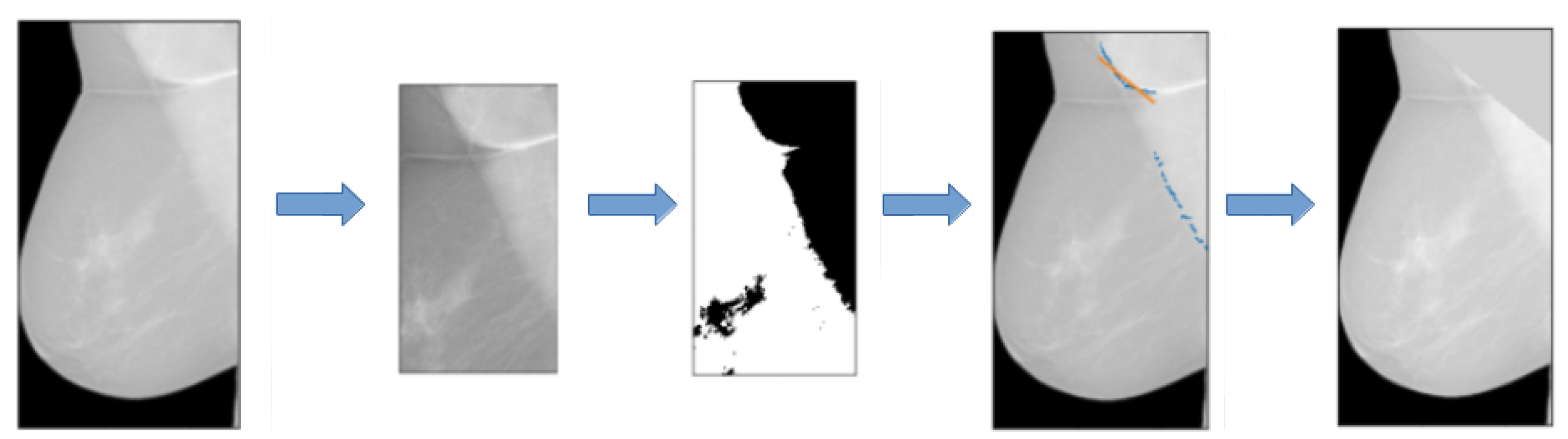
Figure 2.
Main steps describing the pectoral muscle segmentation pipeline.
This procedure works for 80% of the images of our dataset. In Figure 3, we reported an example of a mammogram on which the pectoral muscle segmentation did not achieve a good result. On problematic images, segmentations have been manually fixed, being the robustness of the pectoral muscle segmentation algorithm not one of the main objectives of this work.
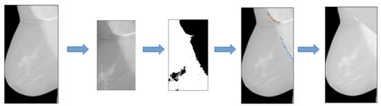
Figure 3.
Example of a mammogram on which the pectoral muscle segmentation did not work properly. The algorithm considers the very first points of the muscle and, as a result, the segmentation does not include the muscle below.
2.2.4. Data Augmentation for CNN Training
The last step of the pre-processing of images for the CNN consists of data augmentation [27]. In fact, although our dataset contains about 6600 images, this amount may not be sufficient to avoid overfitting and to achieve, at the same time, good performances in terms of accuracy [28]. We used the Keras built-in class ImageDataGenerator which applies random transformations to the input data at runtime. The transformations we chose are:
- Random zoom in a range of 0.2;
- Width shift in a range of 0.2 of the whole input image;
- Height shift in a range of 0.2 of the whole input image;
- Random rotations with a range of 10 degrees.
2.2.5. Classifier Training
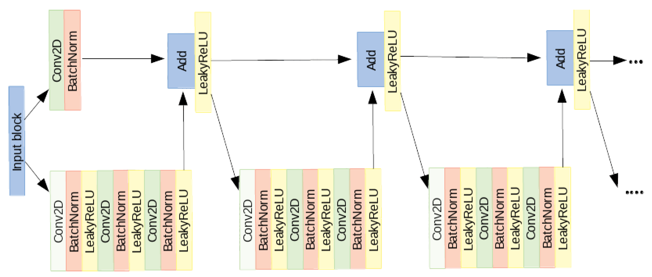
In order to train, fit and evaluate the CNN, Keras -a Python API- with Tensor-flow in backend [29] has been used. We implemented a model based on a very deep residual convolutional neural network [30]. The architecture of our model [21] is made of 41 convolutional layers, organized in residual blocks, and it has about 2 million learnable parameters. The input block consists of a convolutional layer, a batch normalization layer [31], a leakyReLU as activation function and a 2D-max pooling. The output of this block is fed into a series of four blocks, each made of 3 residual modules. In Figure 4, the architecture of one of the four block is shown.

Figure 4.
One of the four blocks made of 3 residual modules.
The input of each of the four blocks is shared by two branches: in the first, it passes through several convolutional, batch normalization, activation and max pooling layers while in the other branch it passes through a convolutional layer and a batch normalization. The outputs of these two branches are then added together to constitute the residual block [30]. The sum goes through a non-linear activation function and the result passes through two identical modules. The architecture of the left branch of these last modules is the same as the first one. In the right branch, instead, no operation is performed. At the exit of the module, the two branches are summed together. At the end of the network, the output of the last block is fed to a global average pooling and to a fully-connected layer with softmax as activation function. We split the data randomly into training set (80%), validation set (10%) and test set (10%). To evaluate the performance, we computed, on the test set, the accuracy, the recall and the precision as figures of merit. They are defined as follows:
where is the number of true-positive, the number of true-negative, the number of false-positive and the number of false-negative detections. The CNN has been trained for 100 epochs and the reported results refer to the epoch with the best validation accuracy. The main hyperparameters are:
- Forty-one convolutional layers organized in 12 similar blocks;
- Training performed in batches of four images;
- Loss function: Categorical Cross-Entropy;
- Optimizer: Stochastic Gradient Descent (SGD);
- Regularization: Batch Normalization;
- Learning rate = 0.1, Decay = 0.1, Patience = 15, Monitor = validation loss.
In order to consider all the four projections related to a subject, four CNNs have been separately trained on each projection, on a K80 Nvidia GPU. Finally, the classification scores (i.e., the CNN output) have been averaged separately for right and left breast and, in case of asymmetry, the higher class has been assigned since breast density is an overall evaluation of the projections and, in clinical practice, the radiologist assigns the higher class to subjects with density asymmetry.
2.2.6. Model Explanation
We aimed to characterize the models in a transparent modality and wanted to create an explanation framework for the outcome of a deep CNN to identify which pixels and salient regions in the image influence the most the final prediction. This was done through off-line visualization techniques, which means analyzing an already trained model without altering its architecture. We used the visualizecam utility function, provided by Keras, to generate a gradient based class activation map that maximizes the outputs of filters within a specified layer and returns an image indicating the regions of the input whose changes would most contribute towards maximizing the output. This function implements a way of visualizing attention over input, which is known as grad-CAM. The basic idea of class activation mapping technique is to identify the importance of image regions by projecting back the weights of the output layer onto the convolutional feature maps. A weighted sum of the feature maps of the last convolutional layer is computed to obtain class activation maps. Grad-CAM uses the gradient information flowing into the last convolutional layer of the CNN to assign importance values to each neuron for a particular decision of interest. In order to obtain the class-discriminative localization map Grad-CAM of width u and height vs. for any class c, we first compute the gradient of the score for class c, (before the softmax), with respect to feature map activations of a convolutional layer, i.e., . These gradients flowing back are global-average-pooled over the width and height dimensions (indexed by i and j, respectively) to obtain the neuron importance weights :
This weight highlights the ‘importance’ of a feature map k for a target class c. Then, a weighted combination of forward activation maps, followed by a ReLU results in:
To sum up, knowing where the gradient is large allows us to define regions with a high impact on the final score decision.
2.2.7. Evaluation of the Explanation Framework
There is no standard procedure to quantify the quality of the saliency maps. The grad-CAM algorithm is usually used to visually assess the correctness of the classification. This means that it is used as an observer-dependent measure. Since the breast density classification is an intensity-based classification, it is possible to directly study the correlation between the mammograms and the saliency maps in order to quantify at least whether there is a monotonic dependence between the images and their explanation. For this reason, we computed the Spearman’s rank correlation between the pre-processed images, which actually contain the information strictly related to the breast density provided in input to the CNN, and their relative saliency maps. Since mammograms are gray-scaled we computed the Spearman’s rank correlation between the pixel intensities and the gray-scaled map intensity values to test whether they are in an increasing monotonic relationship, as we would expect. The value for the perfect increasingly monotonic relationship between two variables is 1.
3. Results
3.1. Evaluation of the Effect of Sample Composition on CNN Training
First, we trained the CNN model with different dataset distributions in order to understand whether it is possible to use the maximum available number of images and how much the probability distribution of classes affects the results. Three different distributions have been considered: the native one of the dataset (A: 12%, B: 29%, C: 48%, D: 11%), which is the distribution of the classes in the original dataset as collected from the AOUP; the BIRADS one (A: 10%, B: 40%, C: 40%, D: 10%), the density class distribution provided in the BIRADS Atlas; and a uniform one (A: 25%, B: 25%, C: 25%, D: 25%), i.e., a distribution including the same proportion of the four density classes. The CNN was trained and tested on samples with these three different distributions of class labels. In Table 2, the performance metrics results are shown.
Table 2.
Final results of CNN trained on different training set and tested on different test sets.
From Table 2, we can observe that the best accuracy, precision and recall in the classification are achieved by training the CNN on the BIRADS distribution of samples (A: 10%, B: 40%, C: 40%, D: 10%) and testing it on the same BIRADS distribution. Moreover, this distribution is the closest to the real data distribution. In fact, it is the one reported in the BIRADS Atlas made on more than 3,800,000 screening examinations and so it is the most representative of what we can observe in clinical practice. Moreover, in our dataset, we have a small number of mammograms of class D. This means that we should have a dataset with a very small total size to have a uniform distribution, and this size is too small to train our deep network. The best performance is achieved when the classifier is trained on a set of images with the BIRADS distributions of classes and tested on a set with the same distribution. Although maintaining the proportion among classes reported in the BIRADS Atlas, representative of the screening practice, forced us to use a reduced dataset size, this did not penalize the results. However, training the network on a dataset with a uniform distribution of the classes, therefore with an even smaller size, gives worse results. We can conclude that the dataset size does affect the obtained results and the probability distribution of classes is an influencing factor as well.
3.2. Implementation and Visual Assessment of the Grad-CAM Technique
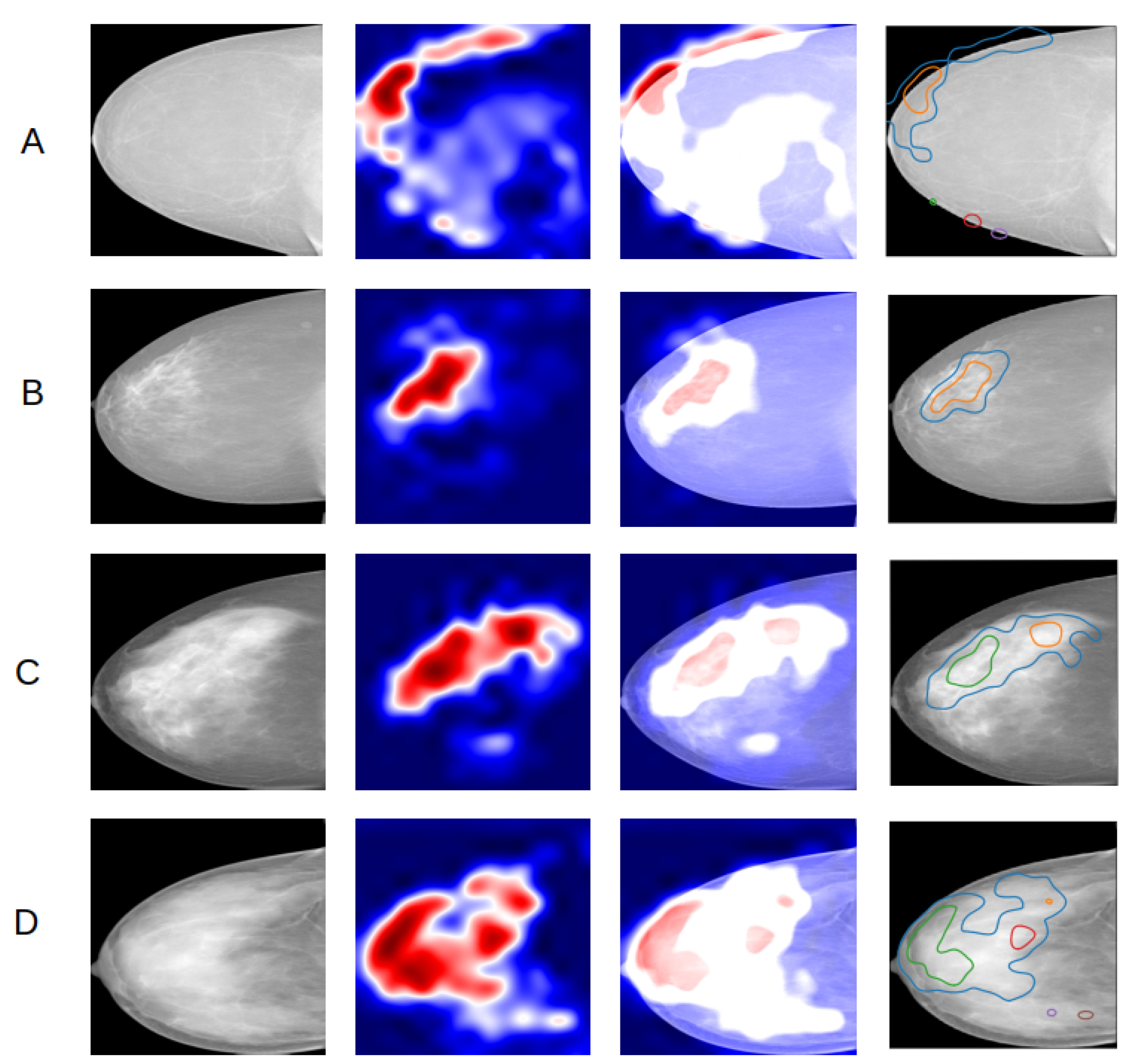
Second, the heatmaps obtained through the grad-CAM technique have been used to establish if the classifier effectively makes its predictions based on the presence of dense areas in the mammogram. This fits into the more general purpose of assessing trust in predictions from our algorithm. The heatmap evaluation has been done qualitatively, which means by visually estimating if the highlighted regions in the heatmap correspond to the denser regions in the original image. The analysis consisted in visualizing and comparing the maps generated using the input images of the four classes. The maps have been produced for all the images in the test set and for all the four projections constituting the mammographic exam. In Figure 5, an example of a comparison of the heatmaps of the four density classes obtained from a model trained on right cranio-caudal projections is reported.
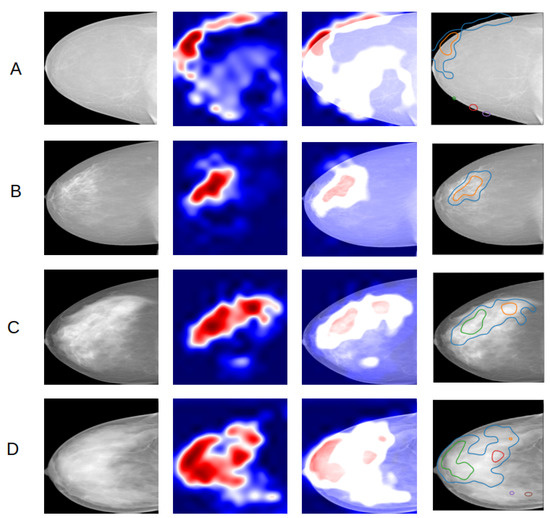
Figure 5.
Comparison of heatmaps of the four density classes (A–D) with one example per class, obtained from a CNN trained on right CC projections. From left to right, the input image, the grad-CAM, the overlay of the map on the input image, the overlay of edges of red activated areas in the map on the input image.
The activated regions in the maps match reasonably well with the dense regions in the original mammogram for B, C and D classes. The grad-CAMs prove that the “attention” of the classifier is focused on the dense region as we expected. An important remark resulting from analyzing all the maps is that for class A mammograms the active area is almost always at the edge of the breast. This is reasonable because the A class is the one corresponding to the lowest density and it seems as if the classifier, not recognizing any dense region, focuses its attention on a different feature, such as the edge.
3.3. Evaluation of the Impact of Pectoral Muscle Removal
Third, we trained the CNN model with and without the pectoral muscle. The images with the pectoral muscle removed have been obtained after applying the algorithm described in Methods section. This algorithm was efficient on 80% of the available exams. The 20% of exams on which the segmentation algorithm failed, i.e., the muscle edge was not correctly identified in at least one projection, were manually segmented. By grad-CAM visualization, we noticed that, for some MLO projection images, the related maps activate at the pectoral muscle visible in these projections. We then trained the CNN on MLO projections with the muscle removed, to check if in this case the classifier performance and the heatmaps improve. In terms of performance metrics, training the model with and without the pectoral muscle gave the results reported in Table 3.
Table 3.
Performances of the CNN trained with images with (with PM) and without the pectoral muscle (without PM).
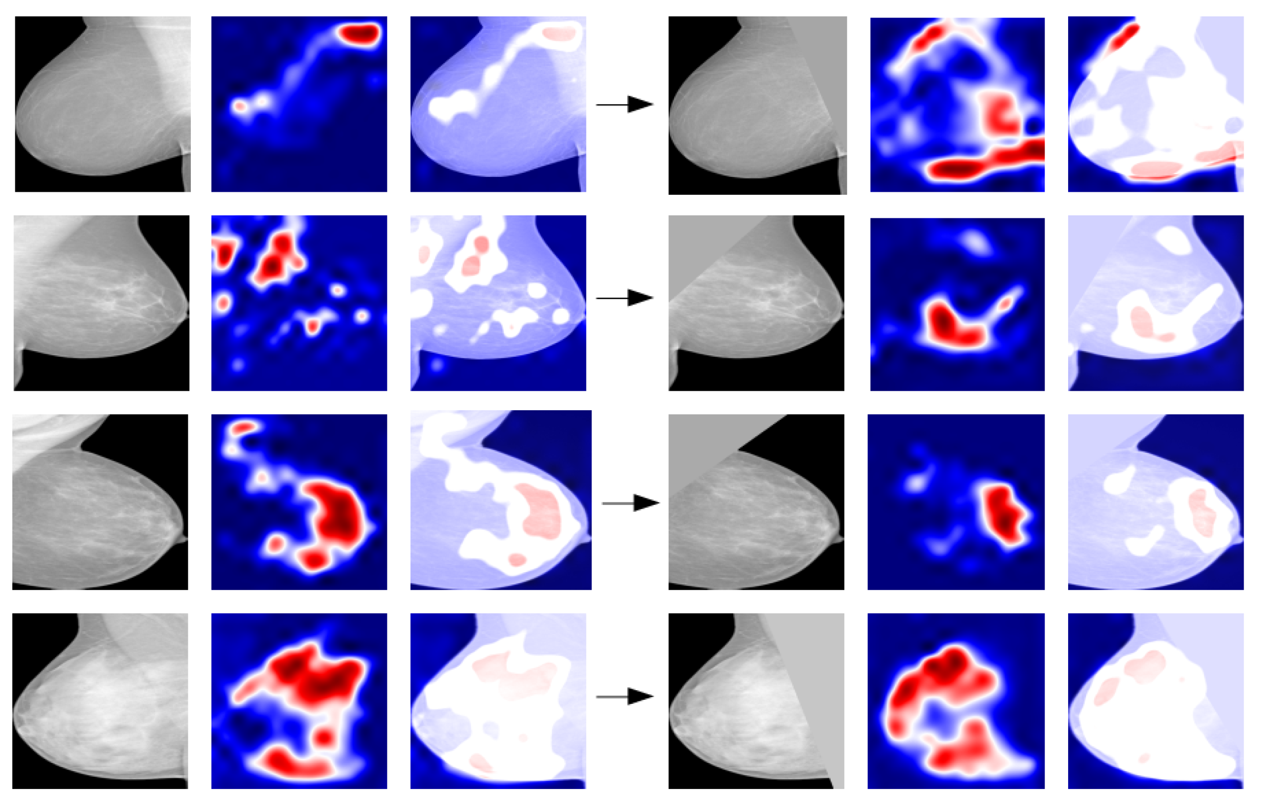
Grad-CAM maps have been generated in the two cases and they have been compared. In most cases, muscle removal helps in guiding the network to focus on the right breast area and after segmentation the pixels forming part of the muscle are no longer highlighted and activated (Figure 6). Therefore, segmentation and removal of pectoral muscle in the image pre-processing phase help in the performance improvement.
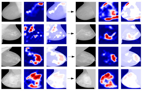
Figure 6.
Example of comparison between grad-CAM maps obtained with the original image (on the left) and with the segmented image (on the right) for various density classes.
3.4. Quantitative Evaluation of the Explanation Framework
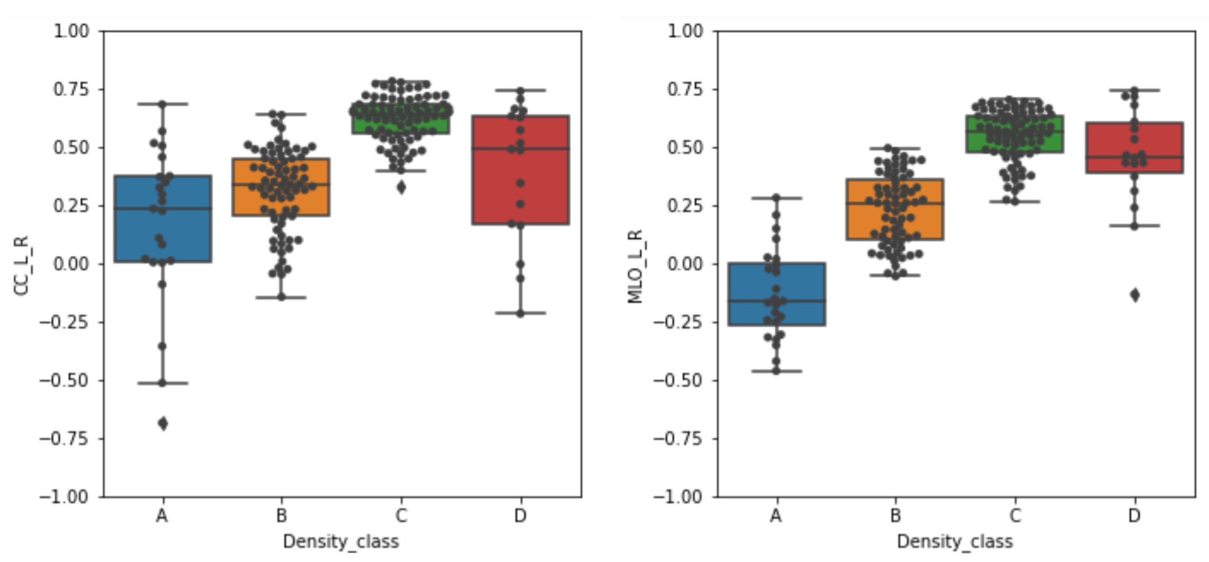
From a visual inspection of a number of examples, including those shown in Figure 6, it seems that to predict the breast density category the CNN is actually “looking” at the appropriate image information, namely the higher-intensity regions of the mammograms. A possibility could be to quantitatively compare the area of the saliency map over a predefined threshold and a hand-crafted pixel-wise ground truth for dense areas generated by a radiologist. That would be an extremely time-consuming task; thus, we discarded this option and proposed a straightforward method to evaluate whether the maps and the higher-density breast areas are spatially correlated. Moreover, for this classification task it is not fair to use pixel wise ground truth since the class assessment by physicians is made by observing the entire image and not pixel wise. It is apparent from a visual inspection of a number of examples, including those shown in Figure 6, that to predict the breast density category the CNN actually relies on an intelligible and appropriate image information, namely the higher-intensity regions of the mammograms. To quantify the extent of this hypothesized direct relationship, we computed the Spearman’s rank correlation coefficient r between the grey-scale image and the grad-CAM map converted into a grey-scale image. The box plots obtained for the correctly classified mammograms in the test set of the four density categories are shown in Figure 7 separately for the CC and MLO projections.

Figure 7.
Box plots of the Spearman’s rank correlation coefficients r obtained for the correctly classified mammograms across the four density categories. The correlation values obtained on the cranio-caudal (CC) and medio-lateral-oblique (MLO) projections are separately shown. The box plots are centered on the median and the boxes represent the interquartile range.
We performed the Kruskal–Wallis test [32], which is a non-parametric ANOVA test, to measure whether there is a significant difference in the Spearman’s rank correlations among the four classes separately for CC and MLO projections. We obtained a p-value less than 0.05 for both tests and, hence, we can affirm that there is a significant difference among the classes. However, the Kruskal–Wallis test does not state if all the groups are significantly different. For this reason we computed the Dunn test [33] with correction for multiple comparisons, which is the post hoc analysis for Kruskal–Wallis test. The Dunn test showed a significant difference among A, B and C classes, while this is not true for the D class (Table 4).
Table 4.
Top: results of the Dunn test, corrected for multiple comparison, computed on CC projections. Bottom: results of the Dunn test, corrected for multiple comparison, computed on MLO projections.
From the boxplots, it can be noticed that high median values of r are generally obtained on mammograms belonging to higher density classes. For the C class the correlation values show the highest median value and the most compact distribution, thus indicating that the CNN classifier is actually considering the higher density areas as the ones to take into account to assign the mammogram to a breast density category. For mammograms of the D class (i.e., those with higher density) this is not always true. The grad-CAM is not in general activated consistently with the higher-density areas of the breast, as depicted in the mammograms. However, the large spread of the r values for this category hampers drawing generalized conclusions. For mammograms of the B categories a positive median r values still indicates a systematic overlap between the higher-intensity areas of the grad-CAM maps and the mammograms. By contrast, the situation is controversial for the mammograms belonging to the A category. In that case, the median r value for CC projection is positive (about 0.25), thus suggesting a systematic overlap between the higher-intensity areas of maps and mammograms, whereas the median r value for MLO projection is negative (about −0.20), thus indicating an opposite relationship. Namely, as visible in the line corresponding to the A example of Figure 6, the grad-CAM map activates in the breast areas complementary to the high-intensity ones. The hypothesized direct monotonic relationship between the pixel intensity values between the original pre-processed breast mammograms and the saliency maps is thus verified in most cases, namely for the higher-density categories (B, C and D) with median r values above 0.25. For the lower-density A category, the behavior of the CNN seems instead to be different in the interpretation of CC and MLO mammograms, exploiting, in the latter case, the complementary density information.
4. Discussion
As regards the comparison with the previous classifier [21] where no pre-processing was implemented, we obtained better results in terms of the figures of merit and activation maps. In fact, the CNN reaches an accuracy of 82.0%. Moreover, the CNN compares very well with the literature [34] where an accuracy of 77% is obtained with a classifier trained on about 60,000 exams. Compared to [12,13], the CNN based classifier achieves better performances in terms of accuracy (respectively 47% and 71.4%). As regards the study by Oliver et al. [14], our classifier works better also in terms of Cohen (Kappa) coefficient on the four classes problem, since we reach a k equal to 0.76 with respect to 0.67. Other studies [35,36] reach better accuracy on the classification of two classes: dense versus non-dense and BI-RADS 2 versus BI-RADS 3, respectively. It is, hence, not possible to compare our results with theirs. In [37], the accuracy on the 4 BI-RADS classes is equal to 98.75% which is higher than the accuracy reached in this work. However, their method is not explained and not explainable. As a general consideration, the comparison with other different methods is not performed on the same dataset, making it not completely fair. Since our breast density classifier was trained on digital mammograms, the method cannot be applied to MIAS and DDSM which contain analog digitized mammograms. Moreover, analog mammography is not used in hospitals anymore.
We found that pre-processing has a crucial impact not only on the accuracy, but also on the explainability of the classifier. In fact, the grad-CAM activation maps showed a good localization capability once the pectoral muscle has been removed from the image. For this reason, we believe that CNN classifiers should be trained on real medical images paying particular attention not only to the classification performances but also to obtaining reasonable activation maps.
As regards the training on different sample compositions, the discussion on the more appropriate strategy to be used in training ML algorithms in case of unbalanced data set is highly debated [38]. Both the balanced and the natural distribution approach can be actually used [39]. We found out that the CNN performs better on the BI-RADS distribution in terms of accuracy, precision and recall. This distribution is the closest to the natural one reported on the BI-RADS Atlas. This result was not unexpected as the native distribution is strongly unbalanced over the density classes, while the uniform one forces us to use far fewer images than the other two. We then visualized the saliency maps computed on the test set to check whether the classifier is looking at the dense part of the breast to perform the classification. We found out that for the medio-lateral oblique projections the saliency maps highlighted more the regions of the pectoral muscle than the dense parenchyma. For this reason, we segmented the pectoral muscle and retrained the classifier. Then, we compared the saliency maps obtained with and without the muscle and we found out that segmentation helps in identifying the correct dense region as shown in Figure 6. Furthermore, the performance in terms of figures of merit increases for the classifier trained with the segmentation. Finally, we computed the Spearman’s rank correlation to assess whether the pre-processed images and the relative saliency maps are in a direct monotonic relationship. We found out a correlation for the B, C and D classes while we obtained a controversial result for the A class. The visual inspection of saliency maps and Spearman’s rank correlation computed for different classes show a mutual accordance with our hypothesis. We underline that it is important to evaluate both visually and quantitatively the maps to reach an optimal performance.
5. Conclusions
In this study, we presented a detailed study of a CNN trained on mammograms in an explainable way. We trained a CNN classifier on a wide set of clinical mammograms to classify them according to breast density and then we implemented an explanation algorithm to explore the CNN behavior on different input data. We evaluated the CNN performance using different distributions of class labels in the training and test sets, and different pre-processing steps, taking into account the accuracy, precision and recall figures of merit, and the saliency maps obtained with the grad-CAM algorithm. This approach can be extended to other medical images in the attempt to provide clinicians with reliable and explainable AI-based decision support tools.
Author Contributions
Conceptualization, F.L. (Francesca Lizzi), C.S. and M.E.F.; Data curation, F.L. (Francesca Lizzi) and C.S.; Formal analysis, F.L. (Francesca Lizzi) and C.S.; Funding acquisition, M.E.F. and A.R.; Investigation, F.L. (Francesca Lizzi) and F.L. (Francesco Laruina); Methodology, F.L. (Francesca Lizzi) and A.R.; Project administration, M.E.F.; Resources, F.L. (Francesco Laruina); Software, C.S.; Supervision, F.L. (Francesca Lizzi), M.E.F. and A.R.; Writing—original draft, F.L. (Francesca Lizzi), C.S., M.E.F. and A.R.; Writing–review & editing, F.L. (Francesca Lizzi), C.S. and F.L. (Francesco Laruina). All authors have read and agreed to the published version of the manuscript.
Funding
This work was carried out with support by INFN (National Institute for Nuclear Physics) in the framework of the experiment AIM (Artificial Intelligence in Medicine). It was also supported by Physics Department of Pisa University and SNS (Scuola Normale Superiore).
Institutional Review Board Statement
The study was conducted according to the guidelines of the Declaration of Helsinki and approved by the Review Board constituted by the Radiologist responsible of the Diagnostic Senology Operative Unit of AOUP and the full professor of the Diagnostic and Interventional Radiology Department of University of Pisa. Ethics Committee approval was waived because it was not necessary for this retrospective study: the collection of negative mammograms started in 2011.
Informed Consent Statement
Informed consent was obtained from all subjects involved in the study.
Data Availability Statement
Image data are not public available, but can be obtained upon request to the authors. A research agreement for their use would be needed.
Acknowledgments
This work has been carried out within the Artificial Intelligence in Medicine (AIM) project (INFN-CSN5, 2019–2021, https://www.pi.infn.it/aim, accessed on 21 December 2021). We aknowledge also Fondazione Pisa, Technological and Scientific Research Sector, for the support to the RADIOMA (2017–2020) project (https://fondazionepisa.it/progetti-finanziati/radiazioni-ionizzanti-in-mammografia-conoscerle-per-limitarle-sviluppo-di-un-indicatore-di-dose-innovativo-in-vista-del-recepimento-della-nuova-direttiva-europea/, accessed on 21 December 2021).
Conflicts of Interest
The authors declare no conflict of interest.
Abbreviations
The following abbreviations are used in this manuscript:
| FFDM | Full Field Digital Mammography |
| ACR | American College of Radiology |
| BI-RADS | Breast Imaging Reporting and Data Systems |
| SVM | Support Vector Machine |
| CNN | Convolutional Neural Network |
| grad-CAM | grad Class Activation Map |
| RADIOMA | Ionizing Radiation in MAmmography |
| AOUP | Azienda Ospedaliero Universitaria Pisana |
| CC | Cranio-Caudal (projection) |
| MLO | Medio Lateral-Oblique (projection) |
| DICOM | Digital Imaging and COmmunication in Medicine |
| PNG | Portable Network Graphics |
References
- Siegel, R.L.; Miller, K.D.; Jemal, A. Cancer statistics, 2019: Cancer Statistics, 2019. CA Cancer J. Clin. 2019, 69, 7–34. [Google Scholar] [CrossRef] [Green Version]
- Løberg, M.; Lousdal, M.L.; Bretthauer, M.; Kalager, M. Benefits and harms of mammography screening. Breast Cancer Res. 2015, 17, 63. [Google Scholar] [CrossRef] [PubMed] [Green Version]
- Dance, D.R.; Christofides, S.; McLean, I.; Maidment, A.; Ng, K. Diagnostic Radiology Physics; Non-Serial Publications, International Atomic Energy Agency: Vienna, Austria, 2014. [Google Scholar]
- The Independent UK Panel on Breast Cancer Screening; Marmot, M.G.; Altman, D.G.; Cameron, D.A.; Dewar, J.A.; Thompson, S.G.; Wilcox, M. The benefits and harms of breast cancer screening: An independent review: A report jointly commissioned by Cancer Research UK and the Department of Health (England) October 2012. Br. J. Cancer 2013, 108, 2205–2240. [Google Scholar] [CrossRef] [PubMed] [Green Version]
- D’Orsi, C. ACR BI-RADS® Atlas, Breast Imaging Reporting and Data System; American College of Radiology: Reston, VA, USA, 2013. [Google Scholar]
- Miglioretti, D.L.; Lange, J.; van den Broek, J.J.; Lee, C.I.; van Ravesteyn, N.T.; Ritley, D.; Kerlikowske, K.; Fenton, J.J.; Melnikow, J.; de Koning, H.J.; et al. Radiation-Induced Breast Cancer Incidence and Mortality From Digital Mammography Screening: A Modeling Study. Ann. Intern. Med. 2016, 164, 205. [Google Scholar] [CrossRef]
- McCormack, V.A. Breast Density and Parenchymal Patterns as Markers of Breast Cancer Risk: A Meta-analysis. Cancer Epidemiol. Biomark. Prev. 2006, 15, 1159–1169. [Google Scholar] [CrossRef] [PubMed] [Green Version]
- Boyd, N.F.; Byng, J.W.; Jong, R.A.; Fishell, E.K.; Little, L.E.; Miller, A.B.; Lockwood, G.A.; Tritchler, D.L.; Yaffe, M.J. Quantitative Classification of Mammographic Densities and Breast Cancer Risk: Results From the Canadian National Breast Screening Study. JNCI J. Natl. Cancer Inst. 1995, 87, 670–675. [Google Scholar] [CrossRef] [PubMed]
- Tyrer, J.; Duffy, S.W.; Cuzick, J. A breast cancer prediction model incorporating familial and personal risk factors. Stat. Med. 2004, 23, 1111–1130. [Google Scholar] [CrossRef] [PubMed] [Green Version]
- Ciatto, S.; Houssami, N.; Apruzzese, A.; Bassetti, E.; Brancato, B.; Carozzi, F.; Catarzi, S.; Lamberini, M.; Marcelli, G.; Pellizzoni, R.; et al. Categorizing breast mammographic density: Intra- and interobserver reproducibility of BI-RADS density categories. Breast 2005, 14, 269–275. [Google Scholar] [CrossRef] [PubMed]
- Kumar, I.; Bhadauria, H.S.; Virmani, J.; Thakur, S. A classification framework for prediction of breast density using an ensemble of neural network classifiers. Biocybern. Biomed. Eng. 2017, 37, 217–228. [Google Scholar] [CrossRef]
- Bovis, K.; Singh, S. Classification of mammographic breast density using a combined classifier paradigm. Med. Image Underst. Anal. 2002, pp. 1–4. Available online: https://citeseerx.ist.psu.edu/viewdoc/download?doi=10.1.1.19.1806&rep=rep1&type=pdf (accessed on 1 November 2021).
- Oliver, A.; Freixenet, J.; Zwiggelaar, R. Automatic Classification of Breast Density. In Proceedings of the IEEE International Conference on Image Processing 2005, Genova, Italy, 14 September 2005; pp. 1258–1261. [Google Scholar]
- Oliver, A.; Freixenet, J.; Marti, R.; Pont, J.; Perez, E.; Denton, E.; Zwiggelaar, R. A Novel Breast Tissue Density Classification Methodology. IEEE Trans. Inf. Technol. Biomed. 2008, 12, 55–65. [Google Scholar] [CrossRef] [PubMed] [Green Version]
- Tzikopoulos, S.D.; Mavroforakis, M.E.; Georgiou, H.V.; Dimitropoulos, N.; Theodoridis, S. A fully automated scheme for mammographic segmentation and classification based on breast density and asymmetry. Comput. Methods Programs Biomed. 2011, 102, 47–63. [Google Scholar] [CrossRef] [PubMed]
- Petroudi, S.; Kadir, T.; Brady, M. Automatic classification of mammographic parenchymal patterns: A statistical approach. In Proceedings of the 25th Annual International Conference of the IEEE Engineering in Medicine and Biology Society (IEEE Cat. No.03CH37439), Cancun, Mexico, 17–21 September 2003; pp. 798–801. [Google Scholar] [CrossRef]
- Litjens, G.; Kooi, T.; Bejnordi, B.E.; Setio, A.A.A.; Ciompi, F.; Ghafoorian, M.; van der Laak, J.A.; van Ginneken, B.; Sánchez, C.I. A survey on deep learning in medical image analysis. Med. Image Anal. 2017, 42, 60–88. [Google Scholar] [CrossRef] [PubMed] [Green Version]
- Kortesniemi, M.; Tsapaki, V.; Trianni, A.; Russo, P.; Maas, A.; Källman, H.E.; Brambilla, M.; Damilakis, J. The European Federation of Organisations for Medical Physics (EFOMP) White Paper: Big data and deep learning in medical imaging and in relation to medical physics profession. Phys. Med. 2018, 56, 90–93. [Google Scholar] [CrossRef] [PubMed] [Green Version]
- Ribeiro, M.T.; Singh, S.; Guestrin, C. “Why Should I Trust You?”: Explaining the Predictions of Any Classifier. arXiv 2016, arXiv:1602.04938. [Google Scholar]
- Suckling, J.; Parker, J.; Dance, D.; Astley, S.; Hutt, I.; Boggis, C.; Ricketts, I.; Stamatakis, E.; Cerneaz, N.; Kok, S.; et al. Mammographic Image Analysis Society (MIAS) Database v1.21; 2015. Available online: https://www.repository.cam.ac.uk/handle/1810/250394 (accessed on 21 December 2021).
- Lizzi, F.; Laruina, F.; Oliva, P.; Retico, A.; Fantacci, M.E. Residual Convolutional Neural Networks to Automatically Extract Significant Breast Density Features. In Computer Analysis of Images and Patterns; Vento, M., Percannella, G., Colantonio, S., Giorgi, D., Matuszewski, B.J., Kerdegari, H., Razaak, M., Eds.; Springer International Publishing: Cham, Switzerland, 2019; pp. 28–35. [Google Scholar]
- Lee, R.S.; Gimenez, F.; Hoogi, A.; Miyake, K.K.; Gorovoy, M.; Rubin, D.L. A curated mammography data set for use in computer-aided detection and diagnosis research. Sci. Data 2017, 4, 170177. [Google Scholar] [CrossRef]
- Sottocornola, C.; Traino, A.; Barca, P.; Aringhieri, G.; Marini, C.; Retico, A.; Caramella, D.; Fantacci, M.E. Evaluation of Dosimetric Properties in Full Field Digital Mammography (FFDM)-Development of a New Dose Index. In Proceedings of the 11th International Joint Conference on Biomedical Engineering Systems and Technologies-Volume 1, Madeira, Portugal, 19–21 January 2018; SciTePress: Setúbal, Portugal, 2018; pp. 212–217. [Google Scholar] [CrossRef]
- Wenger, R. Isosurfaces: Geometry, Topology, and Algorithms; CRC Press: London, UK, 2013; Chapter 2; pp. 17–44. [Google Scholar]
- Maple, C. Geometric design and space planning using the marching squares and marching cube algorithms. In Proceedings of the 2003 International Conference on Geometric Modeling and Graphics, London, UK, 16–18 July 2003; pp. 90–95. [Google Scholar] [CrossRef]
- Pedregosa, F.; Varoquaux, G.; Gramfort, A.; Michel, V.; Thirion, B.; Grisel, O.; Blondel, M.; Prettenhofer, P.; Weiss, R.; Dubourg, V.; et al. Scikit-learn: Machine Learning in Python. J. Mach. Learn. Res. 2011, 12, 2825–2830. [Google Scholar]
- Perez, L.; Wang, J. The effectiveness of data augmentation in image classification using deep learning. arXiv 2017, arXiv:1712.04621. [Google Scholar]
- Shorten, C.; Khoshgoftaar, T.M. A survey on image data augmentation for deep learning. J. Big Data 2019, 6, 60. [Google Scholar] [CrossRef]
- Chollet, F. Keras. 2015. Available online: https://keras.io (accessed on 21 December 2021).
- He, K.; Zhang, X.; Ren, S.; Sun, J. Deep Residual Learning for Image Recognition. arXiv 2015, arXiv:1512.03385. [Google Scholar]
- Ioffe, S.; Szegedy, C. Batch Normalization: Accelerating Deep Network Training by Reducing Internal Covariate Shift. arXiv 2015, arXiv:1502.03167. [Google Scholar]
- Kruskal, W.H.; Wallis, W.A. Use of Ranks in One-Criterion Variance Analysis. J. Am. Stat. Assoc. 1952, 47, 583–621. [Google Scholar] [CrossRef]
- Dunn, O.J. Multiple Comparisons Using Rank Sums. Technometrics 1964, 6, 241–252. [Google Scholar] [CrossRef]
- Lehman, C.D.; Yala, A.; Schuster, T.; Dontchos, B.; Bahl, M.; Swanson, K.; Barzilay, R. Mammographic Breast Density Assessment Using Deep Learning: Clinical Implementation. Radiology 2019, 290, 52–58. [Google Scholar] [CrossRef] [Green Version]
- Gandomkar, Z.; Suleiman, M.E.; Demchig, D.; Brennan, P.C.; McEntee, M.F. BI-RADS density categorization using deep neural networks. Proc. SPIE 2019, 10952, 109520N. [Google Scholar] [CrossRef]
- Mohamed, A.A.; Berg, W.A.; Peng, H.; Luo, Y.; Jankowitz, R.C.; Wu, S. A deep learning method for classifying mammographic breast density categories. Med. Phys. 2018, 45, 314–321. [Google Scholar] [CrossRef]
- Saffari, N.; Rashwan, H.A.; Abdel-Nasser, M.; Singh, V.K.; Arenas, M.; Mangina, E.; Herrera, B.; Puig, D. Fully automated breast density segmentation and classification using deep learning. Diagnostics 2020, 10, 988. [Google Scholar] [CrossRef] [PubMed]
- Johnson, J.M.; Khoshgoftaar, T.M. Survey on deep learning with class imbalance. J. Big Data 2019, 6, 27. [Google Scholar] [CrossRef]
- Weiss, G.M.; Provost, F. Learning When Training Data are Costly: The Effect of Class Distribution on Tree Induction. J. Artif. Intell. Res. 2003, 19, 315–354. [Google Scholar] [CrossRef] [Green Version]

Publisher’s Note: MDPI stays neutral with regard to jurisdictional claims in published maps and institutional affiliations. |
© 2021 by the authors. Licensee MDPI, Basel, Switzerland. This article is an open access article distributed under the terms and conditions of the Creative Commons Attribution (CC BY) license (https://creativecommons.org/licenses/by/4.0/).