Estimation of the Prostate Volume from Abdominal Ultrasound Images by Image-Patch Voting

Abstract

Estimation of the prostate volume with ultrasound offers many advantages such as portability, low cost, harmlessness, and suitability for real-time operation. Abdominal Ultrasound (AUS) is a practical procedure that deserves more attention in automated prostate-volume-estimation studies. As the experts usually consider automatic end-to-end volume-estimation procedures as non-transparent and uninterpretable systems, we proposed an expert-in-the-loop automatic system that follows the classical prostate-volume-estimation procedures. Our system directly estimates the diameter parameters of the standard ellipsoid formula to produce the prostate volume. To obtain the diameters, our system detects four diameter endpoints from the transverse and two diameter endpoints from the sagittal AUS images as defined by the classical procedure. These endpoints are estimated using a new image-patch voting method to address characteristic problems of AUS images. We formed a novel prostate AUS data set from 305 patients with both transverse and sagittal planes. The data set includes MRI images for 75 of these patients. At least one expert manually marked all the data. Extensive experiments performed on this data set showed that the proposed system results ranged among experts’ volume estimations, and our system can be used in clinical practice.

1. Introduction

Prostate volume is a crucial parameter in many clinical practices. It plays an essential role in the diagnosis of benign prostatic hyperplasia (BPH) [1]. BPH is a widespread prostatic disease that affects most aged men [2]. Clinicians use prostate volume while managing lower urinary tract symptoms (LUTS) [3]. Another critical area for prostate volume is the calculation of the Prostate-Specific Antigen Density (PSAD) value to detect and manage prostate cancer (PCa) [4]. PCa was the second most prevalent cancer for the year 2020 and the most prevalent cancer for the last five years among men [5]. PSAD plays a role as one of the criteria for active surveillance decisions in clinical practice [6]. Combining PSAD with other scores may help to decide biopsies [7].

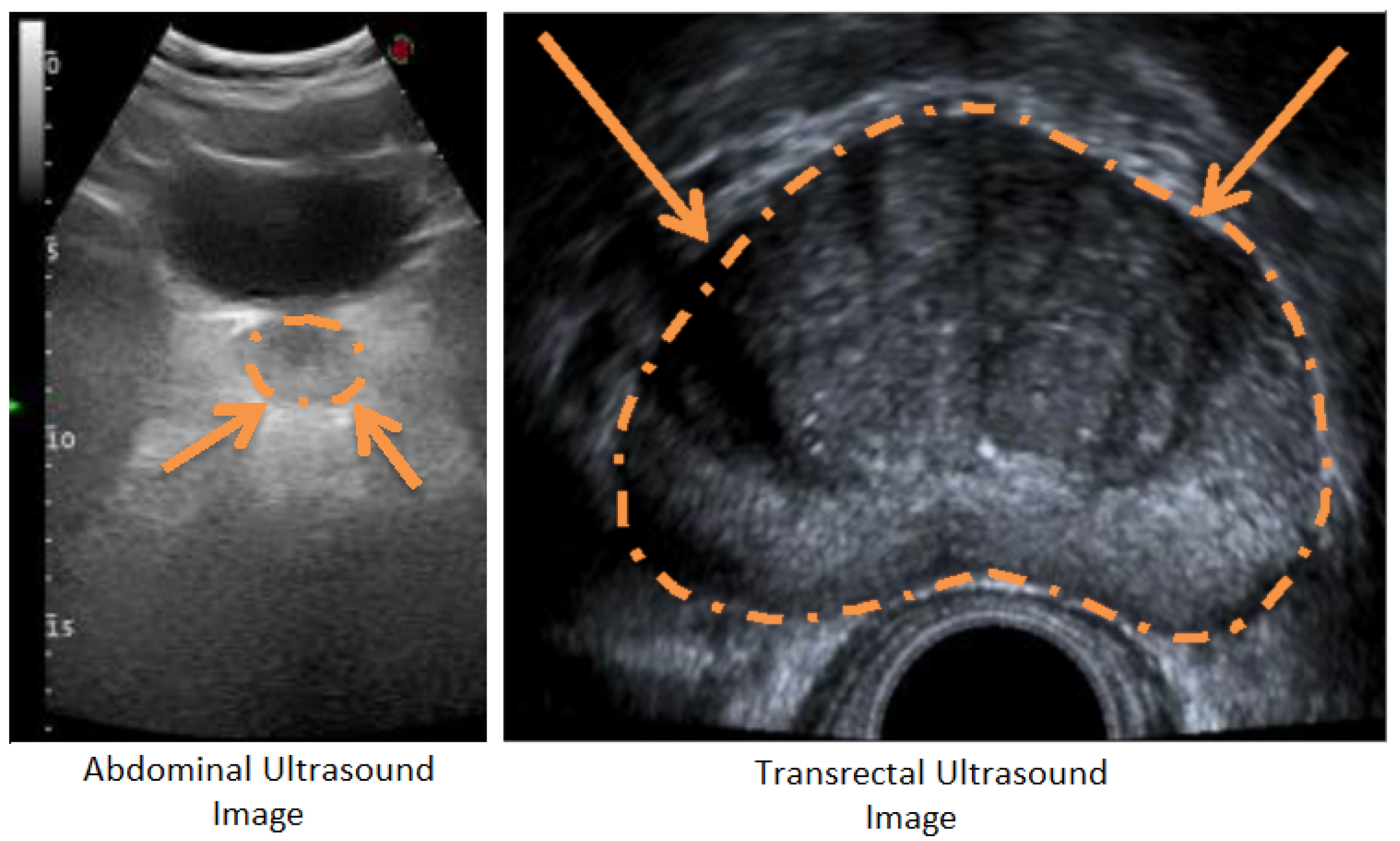
There are many medical-imaging technologies to estimate prostate volume. Widely used technologies are Magnetic Resonance Imaging (MRI), Computed Tomography (CT), and Ultrasound (US) [8]. US technology differs from others with its portability, low-cost, and harmlessness, and it allows experts to scan the prostate in real-time [9]. Trans Rectal Ultrasound (TRUS) and Abdominal Ultrasound (AUS) technologies are frequently used in prostate applications. As shown in Figure 1, despite its better imaging quality with a higher Signal-to-Noise Ratio (SNR) and a larger view of the prostate with no other anatomic structures, TRUS technology is difficult to use regularly during successive radiotherapy sequences [10] due to patient discomfort [11]. The AUS technique is an easy-to-use alternative US imaging technology and is often used where TRUS is not practical.

Conventionally, a prostate-volume measurement is done manually on medical images by experts. Manual volume estimation results in high intra-expert and inter-expert difference due to factors caused by imaging quality, personal experience, and human error [12], which suggests that the guidance of experts by automatic systems would be beneficial. Automated prostate-volume-estimation systems are also essential to reduce the time spent while measuring the prostate volume.

Segmentation and contour extraction methods are used in many studies to infer the prostate volume. However, when AUS images are considered in problems such as low SNR, artifacts and incomplete contours challenge even the state-of-the-art deep-learning techniques. That makes AUS imaging a rarely studied method for automatic prostate-volume measurement systems. This study aimed to demonstrate that an AUS-based automated system for measuring the prostate volume can be an alternative to TRUS, MRI, or CT-based systems.

In our study, we developed a method for estimating prostate volume by following the steps of the standard ellipsoid volume formula, which is not easily applicable in an end-to-end automated system. Our system gives both intermediate and final results, allowing both manual intervention and fully automated employment. To measure prostate volume, we estimated the three major diameters of the ellipsoid representing the prostate. Estimation of diameters was made by detecting four points from transverse and two points from sagittal AUS images. We call these points diameter endpoints. To overcome the characteristic problems of AUS images, we developed a voting-based method to detect points where various locations vote for distance and orientation values relative to each diameter endpoint. We designed a novel network model to carry out the voting process.

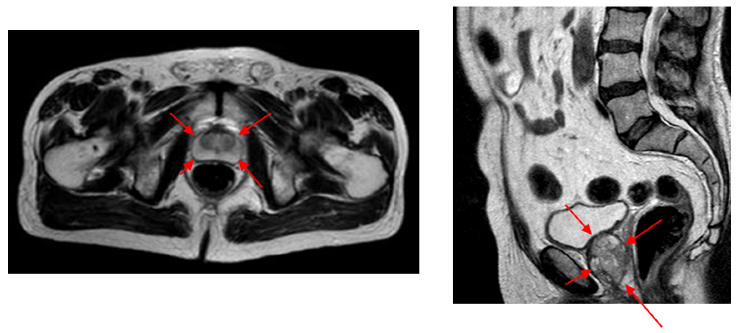
We were unable to compare our volume-estimation results with other studies as almost no other studies are available to estimate prostate volume from AUS images. Instead, we evaluated the difference in intra- and inter-expert volume estimates on AUS images and compared these values with our system estimates. Due to the higher SNR values and better image quality compared (Figure 2) to both AUS and TRUS images (Figure 1), MR image annotations are considered the gold standard [13] in prostate applications. Accordingly, we also evaluated the intra- and inter-expert volume estimation difference in MR images and compared these values with our system’s volume estimations and expert estimations on AUS images. The results show that our system achieved the volume estimate difference values of human experts.

Our novel data set consists of both transverse and sagittal AUS samples from 305 patients. Of these patients, 75 had corresponding MR images from both the transverse and sagittal planes. These AUS and MR images were annotated by several experts during medical treatments. Two experts marked 251 AUS and 73 MR samples at two marking sessions in our experiments. As one of the contributions of our work, this data set is opened to the academic community. We expect this data set to be particularly useful, as, to our knowledge, there is no AUS data set with corresponding MR markings. Supplementary material for this study is added to https://github.com/nurbalbayrak/prostate_volume_estimation (accessed on 23 January 2022).

The rest of this article is organized as follows: Previous work on prostate-segmentation methods on US images is briefly given in Section 2. The proposed method on prostate volume estimation is explained in Section 3. Experiments and results are given in Section 4. The final conclusions and discussions are presented in Section 5.

2. Previous Work

We first briefly review prostate-segmentation methods on US images, as automated prostate volume estimation is primarily performed using segmentation methods. In general, almost all prostate-segmentation studies in the US modality have been performed on TRUS images. To our knowledge, there had been only one study available [10] on AUS images apart from our previous work [14,15]. Therefore, this section will also be a review of prostate segmentation on TRUS images.

Early work on prostate segmentation began with edge-based methods, which often use filters to extract edges from medical images. However, low SNR values in US images caused broken edges, and these algorithms needed to be supported by texture information. Liu et al. [16] used the Radial Bas-Relief (RBR) technique to outline the prostate border. Kwoh et al. [17] used the harmonic method, which eliminates noise and encodes a smooth boundary. Aarnink et al. [18] used the local standard deviation to determine varying homogeneous regions to detect edges. A three-stage method was applied by Pathak et al. [19]. To reduce speckle noise, they first applied a stick filter, then the image was smoothed using an anisotropic diffusion filter, and in the third step, preliminary information such as the shape and the echo model were used. A final step was the manual attachment of the edges, integrating patient-specific anatomical information.

Deformable models were also used in US prostate-segmentation studies and overcame the broken boundary problems in edge-based methods. Deformable models provide a complete contour of the prostate and try to preserve the shape information by internal forces while being placed in the best position representing the prostate border of the image by external forces. Knoll et al. [20] suggested using localized multiscale contour parameterization based on 1D dyadic wavelet transform for elastic deformation constraint to particular object shapes. Ladak et al. [21] required manual initialization of four points from the contour. The estimated contour was then automatically deformed to fit the image better. Ghanei et al. [22] used a 3D deformable model where internal forces were based on local curvature and external forces were based on volumetric data by applying an appropriate edge filter. Shen et al. [23] represented the prostate border using Gabor filter banks to characterize it in a multiscale and multi-orientation fashion. A 3D deformable model was proposed by Hu et al. [24] initialized by considering six manually selected points.

A texture matching-based deformable model for 3D TRUS images was proposed by Zhan et al. [25]. This method used Gabor Support Vector Machines (G-SVMS) on the model surface to capture texture priors for prostate and non-prostate tissues differentiation.

Region-based methods focused on the intensity distributions of the prostate region. Graph-partition algorithms and region-based level sets were used in prostate-segmentation algorithms to overcome the absence of the strong edges problem. A region-based level-set method was used by Fan et al. [26] after a fast-discriminative approach. Zougi et al. [27] used a graph partition scheme where the graph was built with nodes and edges. Nodes were the pixels, and horizontal edges that connect these nodes represented edge-discontinuity penalties.

In classifier-based methods, a feature vector was created for each object (pixels, regions, etc.). A training set was built by assigning each object a class label with supervision. The classifier was trained with the training set and learned to assign a class label to an unseen object. Yang et al. [28] used Gabor filter banks to extract texture features from registered longitudinal images of the same subject. Patient-specific Gabor features were used to train kernel support vector machines and segment newly acquired TRUS images. Akbari et al. [29] trained a set of wavelet support vector machines to adaptively capture features of the US images to differentiate the prostate and non-prostate tissue. The intensity profiles around the boundary were compared to the prostate model. The segmented prostate was updated and compared to the shape model until convergence. Ghose et al. [30] built multiple mean parametric models derived from principal component analysis of shape and posterior probabilities in a multi-resolution framework.

With the development of deep-learning methods, feature-extraction tasks moved from the human side to the algorithm side. This allowed experts in many areas to use deep learning for their studies. Yang et al. [31] formulated the prostate boundary sequentially and explored sequential clues using RNNs to learn the shape knowledge. Lei et al. [32] used a 3D deeply supervised V-Net to deal with the optimization difficulties when training a deep network with limited training data. Karimi et al. [33] trained a CNN ensemble that uses the disagreement among this ensemble to identify uncertain segmentations to estimate a segmentation-uncertainty map. Then uncertain segmentations were improved by utilizing the prior shape information. Wang et al. [34] used attention modules to exploit the complementary information encoded in different layers of CNN. This mechanism suppressed the non-prostate noise at shallow layers and increased more prostate details into features at deep layers of the CNN. Orlando et al. [35] modified the expansion section of the standard U-Net to reduce over-fitting and improve performance.

In our previous work, [14], we implemented a part-based approach to detect the prostate and its bounding box. The system was built on a deformable model of the prostate and adjacent structures. In another previous work, [15], we used concatenated image patches at different scales and trained a model with a single network. There was a voting process for the whole prostate boundary and layers parallel to the boundary. In this study, we extended our previous work to use a new patch mechanism with a new model. Additionally, we have MR annotations corresponding to AUS samples in our experiments, which will be used for comparison with golden volume standard.

Fully automated radiology measurement systems are a topic of discussion in healthcare. Most of these systems are designed in an end-to-end fashion [36,37] that complicates the expert-in-the-loop solutions that are more compatible with experts’ normal workflow. Clinicians often need to know how outputs are produced to trust the system [38]. It is not easy to examine the results of end-to-end systems because they are too complex to be understood and explained by many [39]. The operation of these systems should be transparent so that they can be explained and interpreted by experts [40]. The combination of artificial and human intelligence in medical analysis would outperform the analysis of fully automated systems or humans [41], while being faster than traditional systems [42]. Our model addresses these issues by following the classical prostate-volume-estimation process. The resulting system yields intermediate results that allow manual intervention and are explainable for experts. It also produces final results allowing fully automatic use.

3. Proposed Method

Our study aimed to automate the widely used manual prostate-volume-approximation method that uses the standard ellipsoid volume formula,

$$V(W,H,L)=W.H.L.\pi /6,$$

(1)

where W, H, and L are the width, the height, and the length of the ellipsoid, respectively. The proposed system detects four diameter endpoints from transverse and two from sagittal planes. These locations provide the ellipsoid diameters to obtain W, H, and L values to estimate the prostate volume. We propose an image-patch voting method in which image patches from different locations vote for diameter endpoints.

In this section, we will first talk about the patching process, then we will explain the learning model and the training phase. Finally, we will explain prostate volume inference by patch voting.

3.1. Patch Extraction

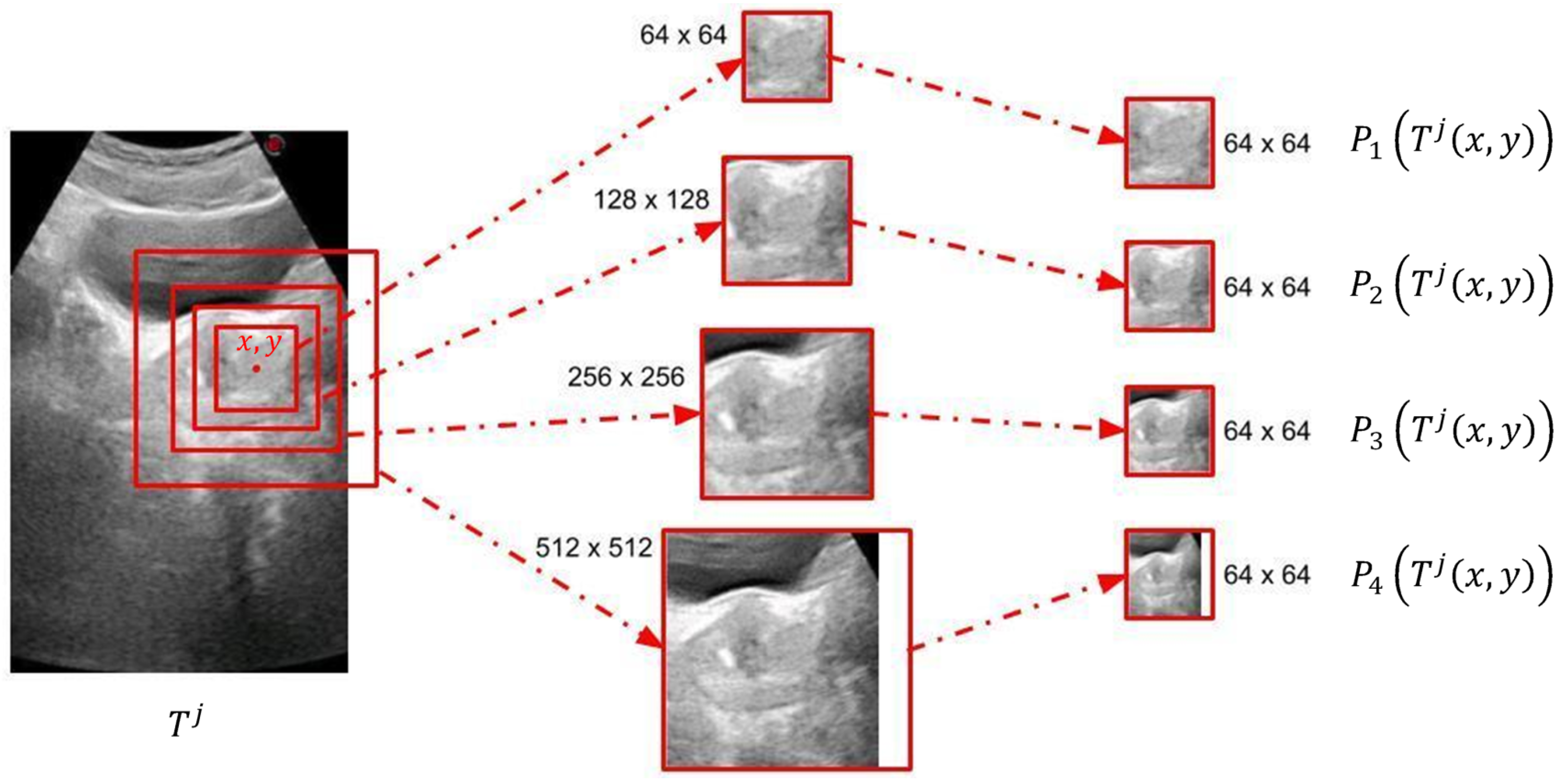
To overcome the characteristic problems of AUS images, we developed an image-patch voting system. Patch-based voting is also useful for augmenting training data. Image-patch voting makes our system robust to noise and prevents it from being affected by unrelated anatomical structures such as the bladder (see Figure 1) by generating a joint solution to the decisions made for patches of many different locations and scales. However, a patch-based system can only extract local information, which may be insufficient for AUS images due to their low SNR values. Therefore, we propose to create multiple patches of different sizes with matching centers to extract information from different scales. As shown in Figure 3, we decided to use four concentric patches, which we call quadruplet patches. The sizes of the patches in our system were $64\times 64$, $128\times 128$, $256\times 256$ and $512\times 512$ pixels. All patches were downsized to $64\times 64$ pixels, except for the smallest scale, which was already $64\times 64$ pixels. The resulting quadruplet patches cast votes for the endpoints of the ellipsoid diameters. For the voting process, we trained a novel neural model explained in Section 3.2.

The locations of the training patches were chosen randomly from a normal distribution around diameter endpoints, while evenly spaced patches were created from test images in a sliding window manner with a stride of 10 pixels. The system extracts 200 patches from each transverse and sagittal image of the training set, which can be considered as an augmentation method that increases size of the training data set. The number of patches extracted from test images changes according to the image size. Sample training patch locations are represented on Figure 4a,b, and test patch locations are represented on Figure 4c,d.

3.2. Quadruplet Network

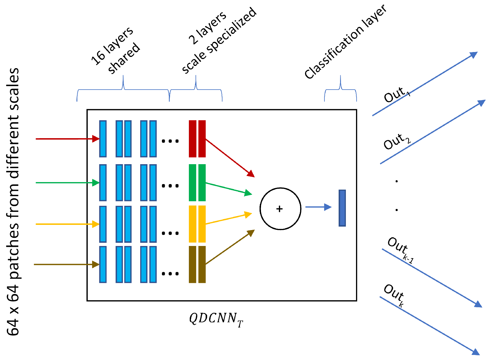
The quadruplet patches described in the previous section vote to estimate diameter endpoints through a network we refer to as Quadruplet Deep Convolutional Neural Network (QDCNN), whose structure is shown in Figure 5. QDCNN comprises four ResNet-18 DCNNs with a joint classification layer and a joint loss. Other types of quadruplet networks are very popular in re-identification or similarity learning studies [43], which are trained with four images where two of them are from the same class, and the others are from different classes. Pairs are learned as positive or negative depending on whether they are in the same or different classes. A quadruplet loss is calculated in this way to achieve greater inter-class and less intra-class variation while identifying images. Differently, in our study, each quadruplet patch obtained at different scales is the input of each of the quadruplet networks with a joint classification layer and a joint loss. The first 16 shared layers of these networks were taken as pretrained from the PyTorch/vision library [44] and frozen, and only the last two layers were fine-tuned during the training process. Thanks to this design, QDCNN can retrieve scale-specific information from each scale.

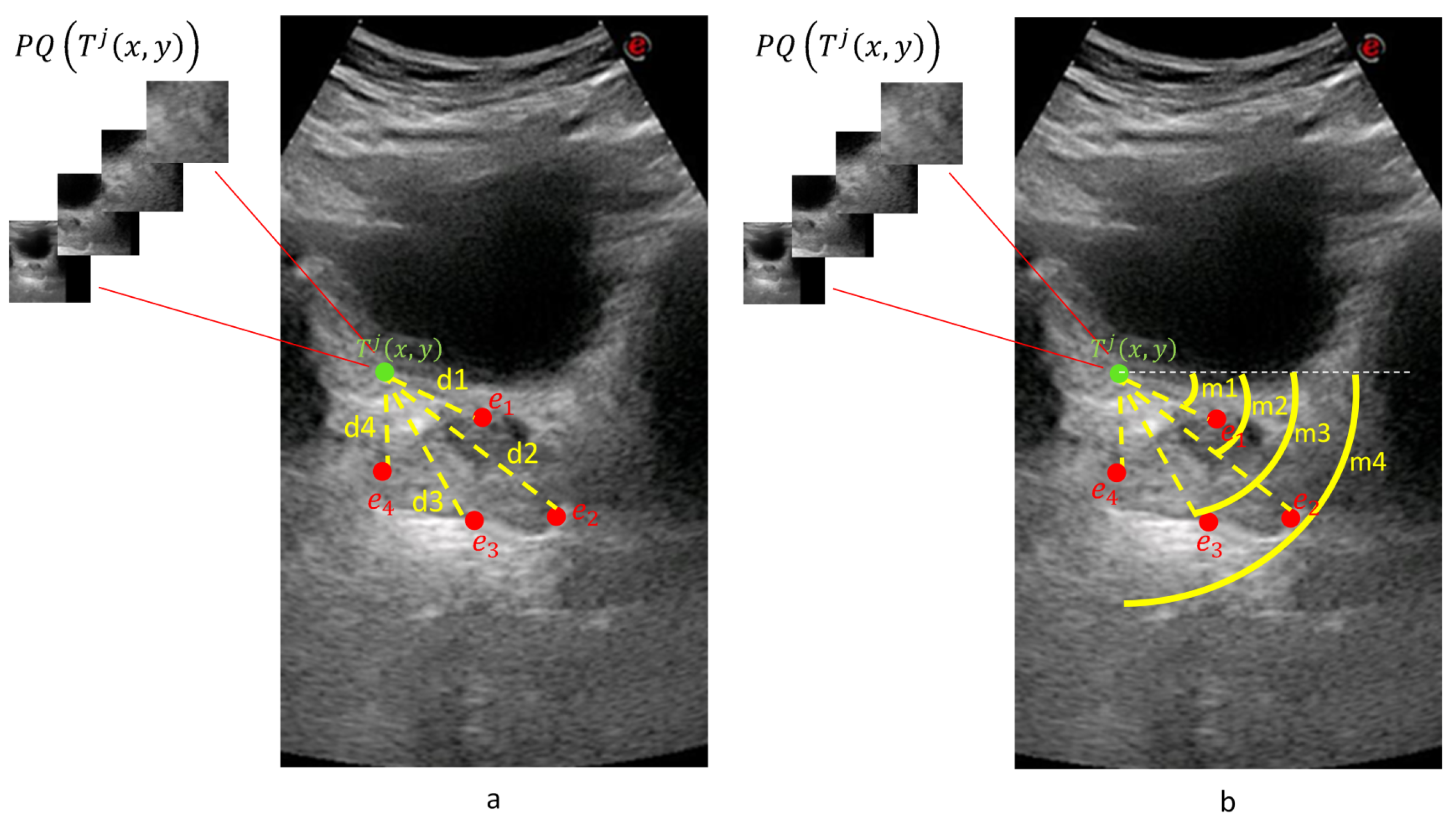
Our quadruplet network is actually a multi-task classifier that learns to predict the distance and orientation classes relative to each diameter endpoint for a given quadruplet patch of a location. Figure 6 shows the calculation of distance and orientation class values. The distance values between 0 and 1000 pixels are quantized into 10 classes, and the 11th class is for values greater than 1000. The intervals for distance classes are smaller for small distance values, and they get larger for larger distances. Orientation values $[0,2\mathrm{\Pi }]$ were quantized into eight equal classes.

Consider the $j^{th}$ patient with a transverse image $T^j$ with diameter endpoints $e_1,e_2,e_3,e_4$ and a sagittal image $S^j$ with diameter endpoints $e_5$ and $e_6$, where $e_i\in R^2$. For a given point $T^j(x,y)$ on the transverse image of the patient j, four equal-size patches $P_1\left(T^j(x,y)\right),P_2\left(T^j(x,y)\right),$$P_3\left(T^j(x,y)\right),$ and $P_4\left(T^j(x,y)\right)$ of different scales were created that composed a quadruplet patch $PQ\left(T^j(x,y)\right)$ of the transverse image. Quadruplet patch $PQ\left(S^j(x,y)\right)$ was created similarly for the sagittal image.

Due to the different structures of transverse and sagittal planes, our system trains two different QDCNN classifiers with a different number of outputs. We defined two functions $c_d$ and $c_o$ to obtain distance ($cd$) and orientation ($co$) classes, respectively. For a given point $T^j(x,y)$ on a given transverse image $T^j$, $c{d}_i^j(x,y)=c_d(T^j(x,y),e_i)$, and $c{o}_i^j(x,y)=c_o(T^j(x,y),e_i)$ where $i=1,\dots ,4$. Similarly, for a given point $S^j(x,y)$ on a given sagittal image $S^j$, $c{d}_i^j(x,y)=c_d(S^j(x,y),e_i)$, and $c{o}_i^j(x,y)=c_o(S^j(x,y),e_i)$ where $i=5,6$. In other words, the QDCNN classifier for the transverse plane (${QDCNN}_T$) has eight classification tasks, and the QDCNN classifier for the sagittal plane (${QDCNN}_S$) has four classification tasks.

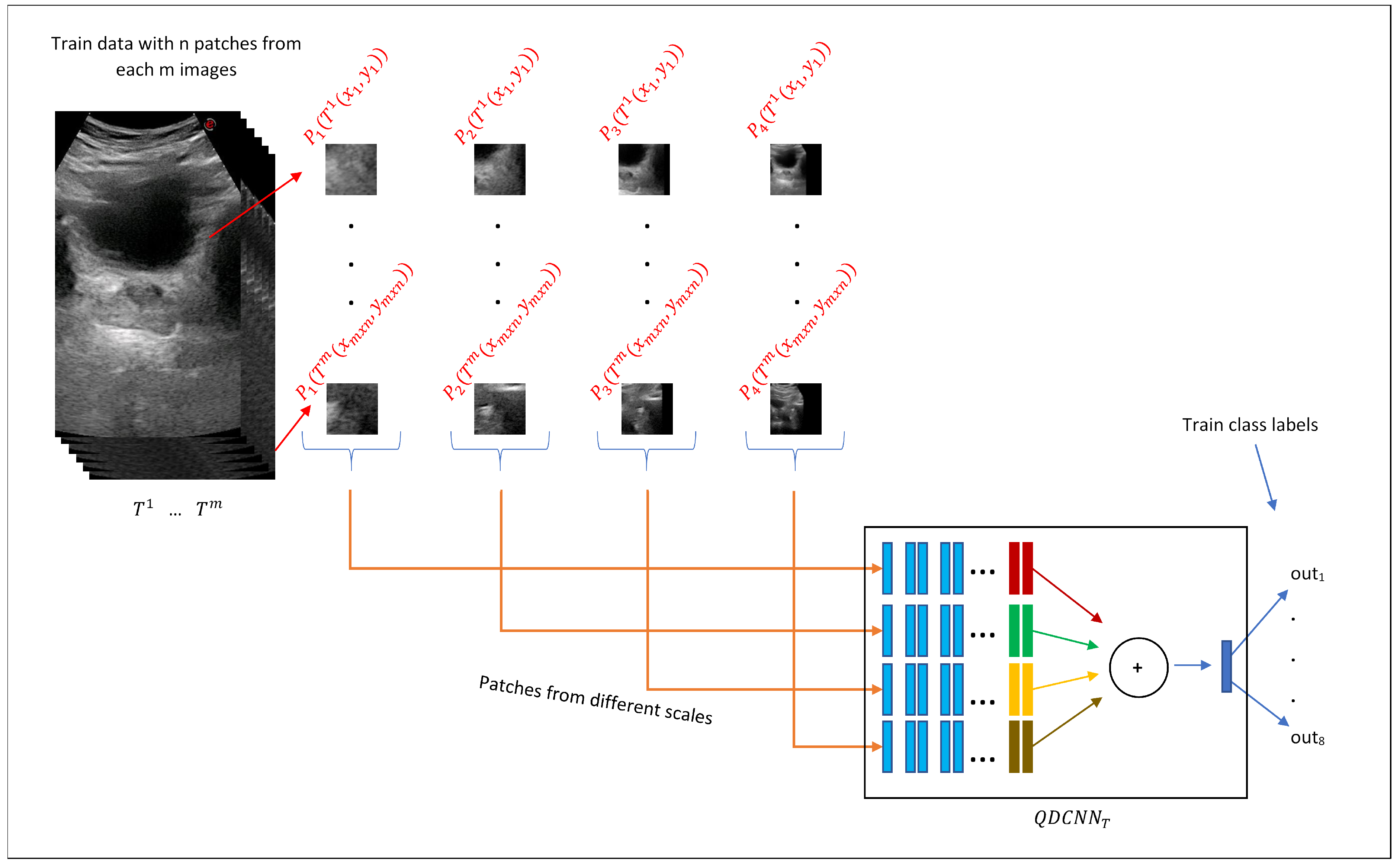
In the training phase, for each AUS image from transverse or sagittal planes, quadruplet patches are extracted from normally distributed random locations around diameter endpoints. Figure 7 demonstrates this process for transverse training images where n quadruplet patches $PQ\left(T^j(x_1,y_1)\right)$,..., $PQ\left(T^j(x_n,y_n)\right)$ were extracted from each of the m transverse training images $T^1,\dots ,T^m$. Then, these quadruplet patches were fed to the ${QDCNN}_T$ for the training process. A similar procedure was followed for the training of the ${QDCNN}_S$ classifier.

3.3. Prostate Volume Inference through Patch Voting

Each quadruplet patch votes for each of the ellipsoid diameter endpoints at the voting space that has the same resolution as the input image. Each quadruplet patch goes through ${QDCNN}_T$ or ${QDCNN}_S$ classifier networks (depending on whether it is extracted from a transverse or sagittal image) to produce $cd$ and $co$ values. The actual voting happens along a circular arc where the arc center is the patch center. The arc radius is given by $cd$ and the arc center angle by $co$. The arc thickness and length are determined by the median and range of the distance and orientation class intervals. This way, a voting map for each diameter endpoint of a given sample is created whose peak gives the location estimation of the diameter endpoint.

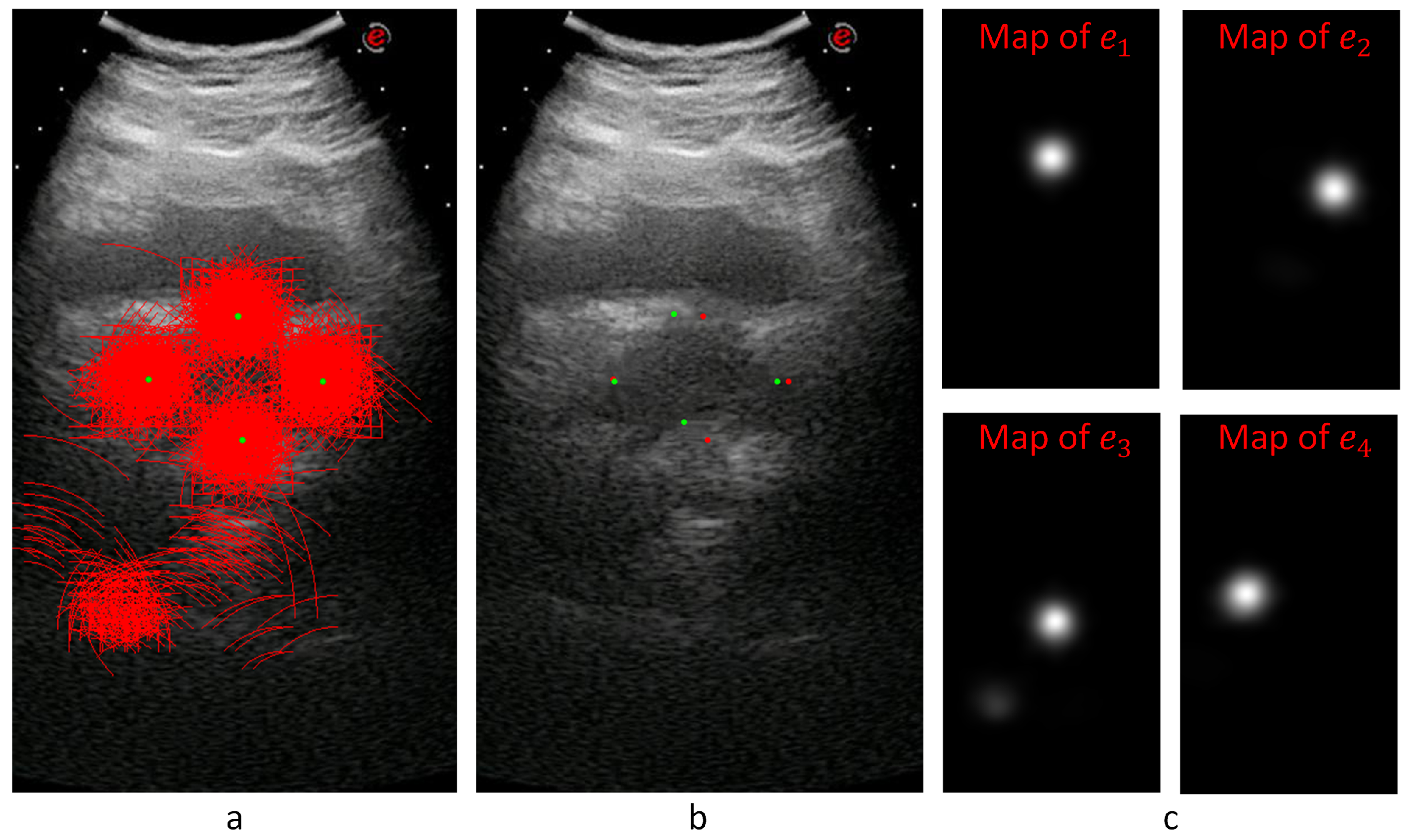
Figure 8 shows an example for the voting maps, arcs, and detected diameter endpoints. In Figure 8a, the arcs are drawn in red with the detected diameter endpoints in green. This sample image does not show the thickness to represent the locations of the arcs better. Figure 8b shows the detected points with red dots, while the manually annotated points are shown with green dots. Figure 8c shows the voting maps of each diameter endpoint. A Gaussian smoothing filter convolves these maps to suppress the noise in these images.

In the test phase, for the transverse $T^j$ and the sagittal $S^j$ images of a given unseen patient j, evenly spaced locations vote for the distance and the orientation class values in a sliding window manner. A quadruplet patch was extracted for each voting location where the quadruplet patch centers the location. The voting process proceeds by the classification of the quadruplet patches by the corresponding QDCNN. Figure 9 exemplifies the voting mechanism on an unseen transverse image $T^j$. For each location $(x,y)$, a quadruplet patch $PQ\left(T^j(x,y)\right)$ was extracted and given as input to the trained $QDCN{N}_T$ classifier to produce eight outputs, which are interpreted as $cd$–$co$ pairs for each of the four endpoints. The final locations of the diameter endpoints were determined as the peaks of the corresponding voting maps. After obtaining the endpoints for the sagittal image $S^j$ similarly, the standard ellipsoid formula was used to estimate the volume.

4. Experiments and Results

In this section, firstly, we will talk about our data set, then we will explain our experiments and give results.

4.1. Data Set and Manual Annotations on AUS and MR Images

Our data set consisted of 305 AUS patient samples with transverse and sagittal images. Of these samples, 75 also had corresponding MR images from transverse and sagittal planes. Manual annotations of these AUS and MR images were done during medical treatments by several experts. The AUS annotations were used to train and test our system, and MR annotations were used as the gold standard.

Of these 305 AUS and 75 MR images, 251 AUS and 73 MR images were annotated by two different experts (exp1 and exp2) at two different marking sessions (mark1 and mark2) within our experiments. These annotations were used to obtain intra-expert and inter-expert volume-estimation differences and to compare expert estimations with our system’s estimations. We defined functions $D_W\left(M\left(T^j\right)\right)$, $D_H\left(M\left(T^j\right)\right)$, and $D_L\left(M\left(S^j\right)\right)$ as the diameters of the width, the height, and the length of the ellipsoid, respectively. M represents the measurement by the experts or the computer. $T^j$ represents transverse and $S^j$ represents sagittal images for the patient j. We calculated the Mean Absolute Value Difference (MAVD) between two different measurements $M_1$ and $M_2$ as

$$MAVD(M_1,M_2)=\frac{1}{N}\sum _{j=1}^N|V_1^j-V_2^j|,$$

(2)

where

$$V_{k=1,2}^j=V(D_W\left(M_k\left(T^j\right)\right),D_H\left(M_k\left(T^j\right)\right),D_L\left(M_k\left(S^j\right)\right))$$

and V is defined in Equation (1). $N=251$ when both of the measurements are from AUS images, and $N=73$ when at least one of the measurements is from a MR image. The top eight rows of

Table 1. Top part shows intra-expert and inter-expert MAVD values in cm${}^3$ for AUS and MR modalities and is symmetrical. The MAVD values between experts, our QDCNN system, and the baseline is shown in the bottom part. Green shows the smallest (best), and red shows the highest MAVD. See the text for the explanation of the column and row headings.

$\mathit{MEAN}$	${\mathit{AUS}}_{\mathit{exp}1}^{\mathit{mark}1}$	${\mathit{AUS}}_{\mathit{exp}1}^{\mathit{mark}2}$	${\mathit{AUS}}_{\mathit{exp}2}^{\mathit{mark}1}$	${\mathit{AUS}}_{\mathit{exp}2}^{\mathit{mark}2}$	${\mathit{MR}}_{\mathit{exp}1}^{\mathit{mark}1}$	${\mathit{MR}}_{\mathit{exp}1}^{\mathit{mark}2}$	${\mathit{MR}}_{\mathit{exp}2}^{\mathit{mark}1}$	${\mathit{MR}}_{\mathit{exp}2}^{\mathit{mark}2}$
${AUS}_{exp1}^{mark1}$		3.46	5.19	5.44	7.70	7.20	6.36	7.12
${AUS}_{exp1}^{mark2}$	3.46		4.76	4.89	8.67	7.96	6.43	7.06
${AUS}_{exp2}^{mark1}$	5.19	4.76		4.01	9.53	9.08	7.15	8.05
${AUS}_{exp2}^{mark2}$	5.44	4.89	4.01		9.68	9.26	6.93	7.38
${MR}_{exp1}^{mark1}$	7.70	8.67	9.53	9.68		2.63	4.96	5.48
${MR}_{exp1}^{mark2}$	7.20	7.96	9.08	9.26	2.63		4.79	4.92
${MR}_{exp2}^{mark1}$	6.36	6.43	7.15	6.93	4.96	4.79		3.00
${MR}_{exp2}^{mark2}$	7.12	7.06	8.05	7.38	5.48	4.92	3.00
${AUS}_{QN}$	4.86	4.52	5.08	5.37	7.10	6.55	5.37	5.86
${AUS}_{BL}$	6.62	6.13	5.79	6.46	7.92	7.27	5.97	5.77

show intra-expert and inter-expert MAVD values of manual prostate-volume-estimations from AUS and MR images. The respective standard deviation values are shown in

Table 2. The corresponding SDAVD values of Table 1.

$\mathit{MEAN}$	${\mathit{AUS}}_{\mathit{exp}1}^{\mathit{mark}1}$	${\mathit{AUS}}_{\mathit{exp}1}^{\mathit{mark}2}$	${\mathit{AUS}}_{\mathit{exp}2}^{\mathit{mark}1}$	${\mathit{AUS}}_{\mathit{exp}2}^{\mathit{mark}2}$	${\mathit{MR}}_{\mathit{exp}1}^{\mathit{mark}1}$	${\mathit{MR}}_{\mathit{exp}1}^{\mathit{mark}2}$	${\mathit{MR}}_{\mathit{exp}2}^{\mathit{mark}1}$	${\mathit{MR}}_{\mathit{exp}2}^{\mathit{mark}2}$
${AUS}_{exp1}^{mark1}$		3.67	5.38	8.35	6.97	6.29	5.32	5.33
${AUS}_{exp1}^{mark2}$	3.67		5.03	7.70	8.05	7.21	5.88	5.75
${AUS}_{exp2}^{mark1}$	5.38	5.03		7.56	10.51	9.68	7.49	6.73
${AUS}_{exp2}^{mark2}$	8.35	7.70	7.56		10.68	9.71	6.92	6.50
${MR}_{exp1}^{mark1}$	6.97	8.05	10.51	10.68		2.63	6.01	5.92
${MR}_{exp1}^{mark2}$	6.29	7.21	9.68	9.71	2.63		4.83	5.16
${MR}_{exp2}^{mark1}$	5.32	5.88	7.49	6.92	6.01	4.83		2.60
${MR}_{exp2}^{mark2}$	5.33	5.75	6.73	6.50	5.92	5.16	2.60
${AUS}_{QN}$	5.70	5.05	5.46	8.12	9.15	7.88	6.51	5.25
${AUS}_{BL}$	7.46	7.12	5.98	8.90	11.17	10.07	7.36	7.09

. The column and the row headings of the top part are defined as $I{T}_e^k$ and represent the modality or the image type $(IT=AUS,MR)$, the expert ID $(e=exp1,exp2)$, and the annotation session ID $(k=mark1,mark2)$.

Table 1 shows that the average intra-expert MAVD values for MR images was 2.81 ($\frac{2.63+3.00}{2}$) cm${}^3$, while it was 3.73 ($\frac{3.46+4.01}{2}$) cm${}^3$ for AUS images. These results show that human experts’ volume estimations can vary at different marking sessions, even for the MR modality, which is the gold standard. It is expectedly normal that there is a greater intra-expert MAVD for the AUS modality due to lower SNR values and other image-quality problems.

The average intra-expert MAVD was 7.63 ($\frac{7.70+7.20+8.67+7.96+7.15+8.05+6.93+7.38}{8}$) cm${}^3$ between the modalities MR and AUS. Considering MR annotations as the gold standard, we can see that manual AUS annotations cause greater MAVD values.

When examining inter-expert MAVD values, we encountered greater values for both intra-modality and inter-modality comparisons. As shown in Table 1, we obtained average values of 5.03 ($\frac{4.96+5.48+4.79+4.92}{4}$) and 5.07 ($\frac{5.19+5.44+4.76+4.89}{4}$) cm${}^3$ inter-expert MAVD for MR-MR and AUS-AUS comparisons, respectively. That shows us that manual annotations by different experts cause greater MAVD for both MR and AUS modalities. When we considered different modalities for inter-expert MAVD, we obtained an average of 8.06 ($\frac{6.36+7.12+6.43+7.06+9.53+9.08+9.68+9.26}{8}$) cm${}^3$ value from which we inferred that manual annotations have a high MAVD between AUS images and the gold standard.

The comparison of the manually marked images shows that there is always a difference between different experts. Similarly, the same expert will mark different positions at different marking sessions. As a result, besides other benefits mentioned before, the guidance of the automated system is expected to enhance the consistency and the stability of the volume-estimation results by the experts. The following section shows our system’s guidance ability, comparing the system and the expert volume estimations.

4.2. Comparison of the Experts, Baseline, and the QDCNN Results

We evaluated our system by 10-fold cross-validation on our data of 305 AUS images. To eliminate any scale differences between images, we re-sampled each image to a 40 pixel/cm scale using the pixel sizes that are always available from the US device.

The second row from the bottom of Table 1 (${AUS}_{QN}$) shows the MAVD values between our QDCNN system and the experts. Comparing our system volume estimations with expert volume estimations on AUS images, we obtained a 4.95 ($\frac{4.86+4.52+5.08+5.37}{4}$) cm${}^3$ average MAVD value, which is smaller than the average inter-expert MAVD value (5.09 cm${}^3$) on AUS images. Overall, we can see that our system’s volume estimations rank among inter-expert comparisons on AUS images. Table 2 shows the Standard Deviation of Absolute Value Difference (SDAVD) values, respectively. We observe from this table that generally for small absolute-value differences, we see smaller standard deviation values for both manual and automated measurements. In other words, our system’s estimations can be considered as stable as the manual estimations.

To evaluate our system’s volume estimations with respect to the gold standard, we compared our system’s volume estimations with expert volume estimations on MR images and obtained 6.22 ($\frac{7.10+6.55+5.37+5.86}{4}$) cm${}^3$ average MAVD, which is less than both the intra-expert (7.63 cm${}^3$) and inter-expert (8.06 cm${}^3$) average MAVD between different modalities (AUS versus MR). We can conclude that experts could possibly produce more consistent and accurate volume estimations under the guidance of our system than the complete manual-annotation method.

In order to compare our system’s performance against the more traditional deep-learning systems, we implemented a baseline system that accepts 300 × 600 pixels AUS images as input and produces the diameter endpoint location estimations as the output. We modified state-of-the-art DenseNet121 [45] to produce the endpoint locations. The baseline system differs from our QDCNN with its single-network non-voting structure. The training data set for the baseline system was augmented by random cropping. The comparison between our system and the baseline model shows the advantages of our image-patch voting numerically, which is demonstrated by Table 1’s last row (${AUS}_{BL}$). We obtained an average of 6.73 ($\frac{7.92+7.27+5.97+5.77}{4}$) cm${}^3$ MAVD between the baseline system and experts on MR images. Similarly, an average of 6.25 ($\frac{6.62+6.13+5.79+6.46}{4}$) cm${}^3$ MAVD was observed between the baseline system and experts on AUS images. Comparing these MAVD values with the values of our system, one can conclude that the image-patch voting technique improves the overall results.

4.3. Ablation Study

We performed an ablation experiment with a subset of our data set. Instead of using all four patch scales, we used patches with pixel sizes ($64\times 64$) and ($128\times 128$). For each patch size, we trained a ResNet-18 network for the transverse and another one for the sagittal plane. In addition, we trained a Twin Deep Convolutional Neural Network (TDCNN) for the transverse and another one for the sagittal plane. A TDCNN is similar to the QDCNN but contains two DCNNs and gets two patches as inputs with sizes ($64\times 64$) and ($128\times 128$) pixels. The model outputs were the $cd$ and the $co$ values for each endpoint.

The patch sizes we used for the ablation study were smaller than the prostate sizes in our data set. Thus, these patch sizes allow us to observe the effect of the quadruplet patch structure, which consists of patches both smaller and larger than the prostate.

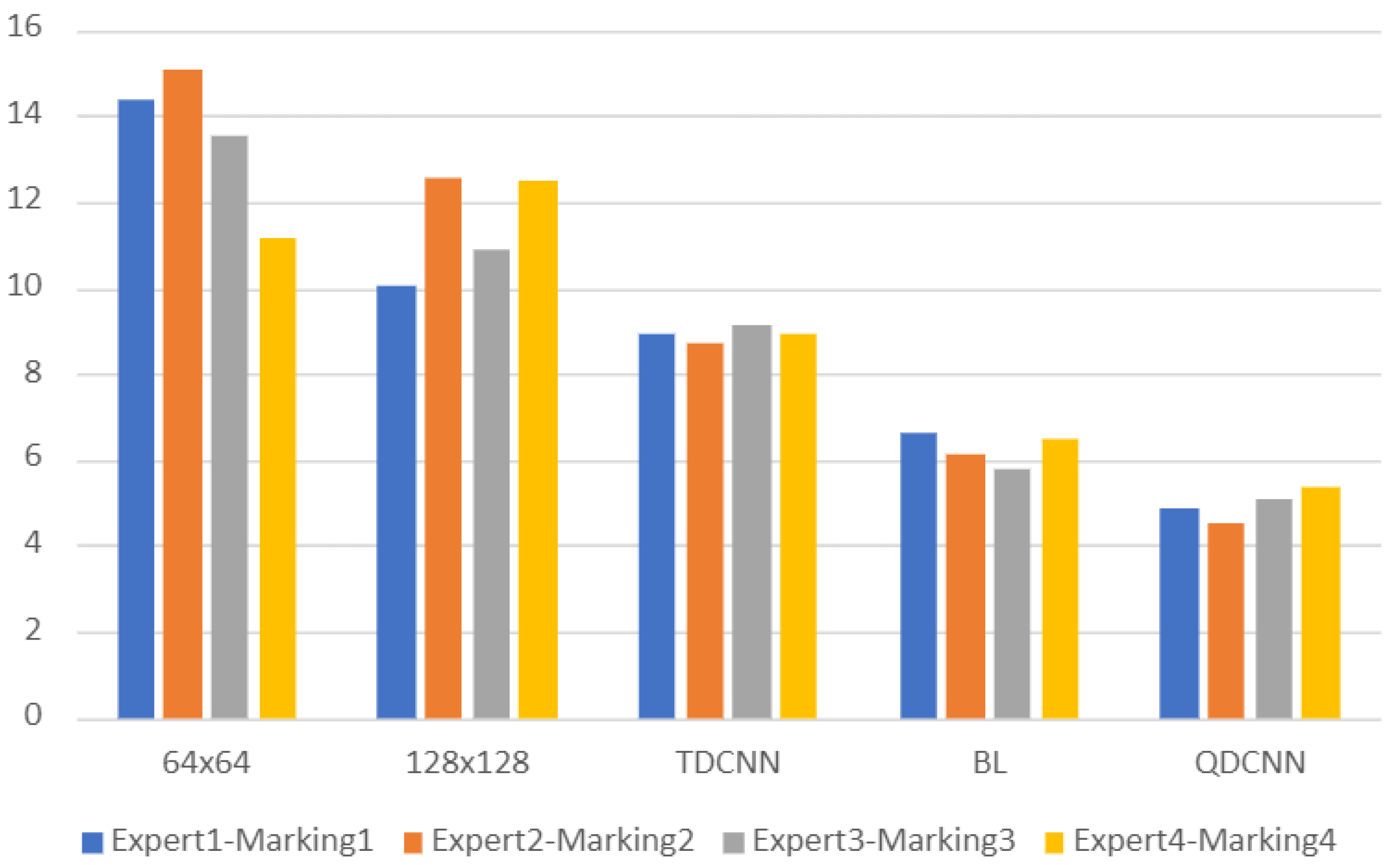
We compared the volume estimations of these individual ResNet-18 networks and TDCNN with the volume estimations of experts on AUS images. The average MAVD between experts and these models were 13.5 cm${}^3$ for the $64\times 64$ ResNet-18 network, 11.4 cm${}^3$ for the $128\times 128$ ResNet-18 network, and 8.92 cm${}^3$ for the TDCNN. Figure 10 shows a bar chart where each group of bars show MAVD values between two different markings of two experts and a model. The first three models are the models of the ablation study. The fourth model is the baseline model, and the last model is the model of the proposed system. The proposed system, QDCNN, has the best MAVD values, which shows the effect of the quadruplet patches and the quadruplet model. TDCNN has better MAVD values than single networks, but it cannot achieve the MAVD values of the baseline system. These MAVD values of the TDCNN show us that using patches only smaller than the prostate is not enough to obtain results ranging among experts.

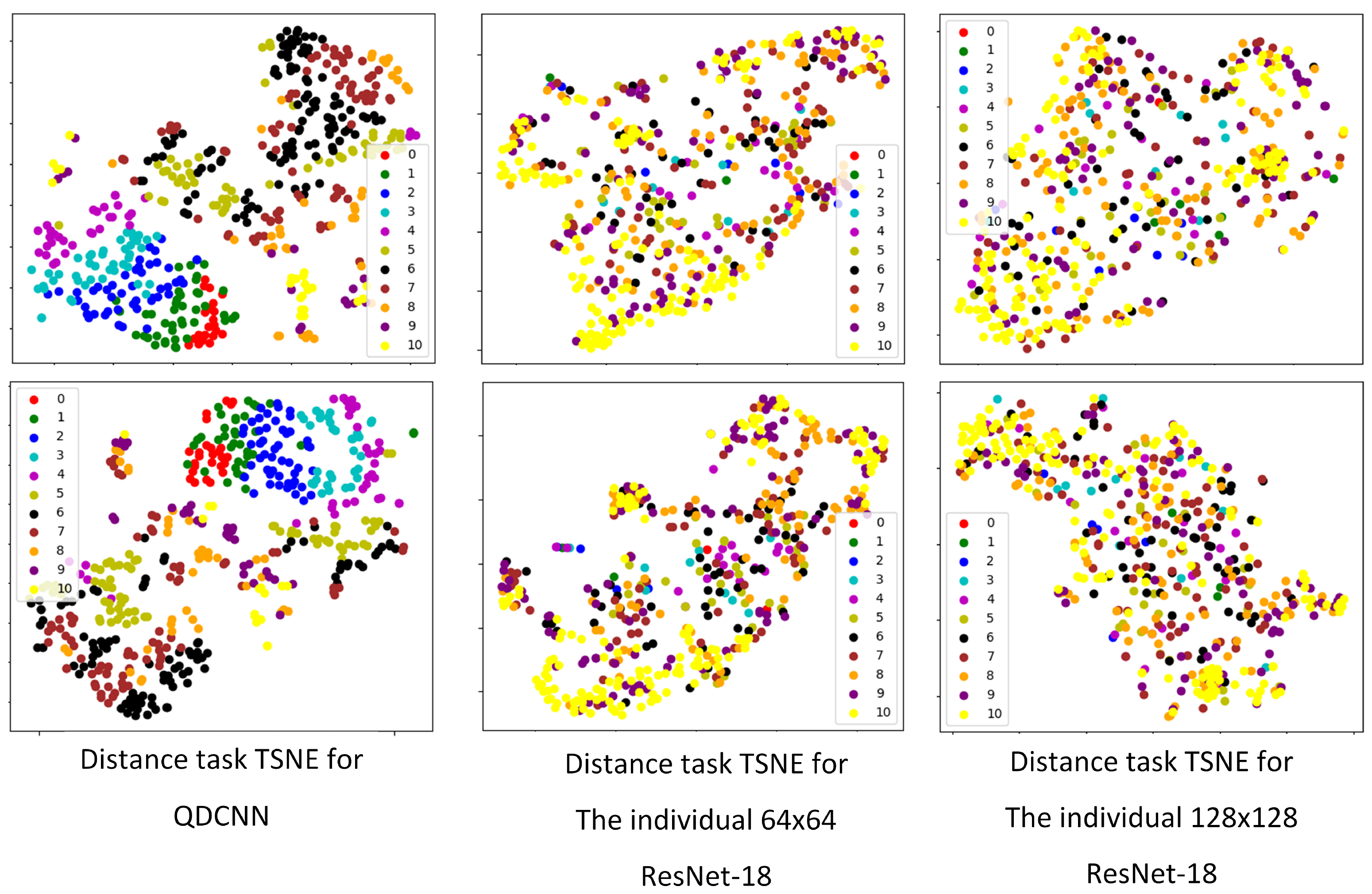
Feature extraction is one of the usage areas of convolutional neural networks [46]. It is known that good deep classifiers can also be used as good feature extractors because good classification results can only come from good features. Thus, we examined the feature-extraction ability of the proposed QDCNN by visualizing the outputs of the last layer before the classification layer of our network as a feature vector. We visualized the feature vectors of the distance tasks for the QDCNN, the individual $64\times 64$ ResNet-18, and the individual $128\times 128$ ResNet-18. We used t-SNE graphs [47] for 2D visualization, and Figure 11 shows two examples of distance tasks for each network. Each color represents a distance class, and each colored point represents a feature vector. The color charts in each graph shows colors associated with class numbers. Smaller numbers show shorter distances, while larger numbers show longer distances. We observed that the class values, especially for the small distances, are nicely separated and grouped together for the quadruplet network. The same grouping cannot be observed for the single-scale networks. These visual results indicate the quality of the features extracted by our network.

5. Conclusions

Radiologists often desire computerized radiology systems with an expert-in-the-loop structure in their everyday workflow, but the popular end-to-end systems are difficult to adapt for such employment. We proposed an image-patch voting system to automate the commonly used ellipsoid formula-based prostate-volume-estimation method. Experts can see the detected endpoints of the ellipsoid diameters and change the endpoint positions if necessary, providing explainability and confidence in the final measurement results. We verified the effectiveness of the image-patch voting method against a common baseline model.

Since some of our sample patients had both AUS and MR images, we had the chance to compare our system’s AUS volume estimations with the gold standard. By comparing both our system and experts to the gold standard, we showed that our system’s volume estimations fall within the expert estimations. The markings made by two experts in two different marking sessions showed unignorable intra-expert and inter-expert MAVD values in the estimations made on both the same and different modalities. On the other hand, the MAVD values of our system, which were less than inter-expert MAVD values on AUS images and intra- and inter-expert MAVD values on different modalities, indicate the good level of guidance ability of the proposed method. Our system can help to enhance expert volume estimations’ stability and consistency.

The new data set we created is valuable for further work on AUS images in automated medical-image analysis. To our knowledge, the data set is the first to include expert markings on both AUS and MR images of sample patients in two different marking sessions. Supplementary material, including the data set, the expert markings, and the project code, is available for public use at https://github.com/nurbalbayrak/prostate_volume_estimation (accessed on 23 January 2022).

Future work might apply the proposed model and patch structure to other modalities. Hybrid modalities [48] might be a good supply of data for a multi-patch system like the proposed one. Statistical analysis might be done to test statistical MAVD differences among different groups.