Abstract
The acoustic emission (AE) technique has become a well-established method of monitoring structural health over recent years. The sensing and analysis of elastic AE waves, which have involved piezoelectric wafer active sensors (PWAS) and time domain and frequency domain analysis, has proven to be effective in yielding fatigue crack-related information. However, not much research has been performed regarding (i) the correlation between the fatigue crack length and AE signal signatures and (ii) artificial intelligence (AI) methodologies to automate the AE waveform analysis. In this paper, this crack length correlation is investigated along with the development of a novel AE signal analysis technique via AI. A finite element model (FEM) study was first performed to understand the effects of fatigue crack length on the resulting AE waveforms and a fatigue experiment was performed to capture experimental AE waveforms. Finally, this database of experimental AE waveforms was used with a convolutional neural network to build a system capable of performing automated classification and prediction of the length of a fatigue crack that excited respective AE signals. AE signals captured during a fatigue crack growth experiment were found to match closely with the FEM simulations. This novel AI system proved to be effective at predicting the crack length of an AE signal at an accuracy of 98.4%. This novel AI-enabled AE signal analysis technique will provide a crucial step forward in the development of a comprehensive structural health monitoring (SHM) system.
1. Introduction
For engineering structures in service, safety and trustworthiness are of the utmost concern. In the numerous different operation modes that engineering structures are exposed to, there exist various types of possible failure mechanisms. In metals, common damage cases include fatigue, static failure, and friction each of which may result depending on the loading and working conditions to which the metal structures are exposed. The number of fatigue-prone structures in current and future engineering applications continues to grow, yielding the demand for a robust and efficient method of monitoring their structural integrity during operational use. The structural health monitoring (SHM) field is an emerging methodology that is used as a technique for detecting damages in structures, such as fatigue damage [1,2,3]. In general, the SHM approach involves the installation of sensors to collect pertinent data, enabling decisions on structure reliability and remaining life [4]. The SHM technique/process, in general, can be described in four levels. These levels explain how, from start to finish, an SHM system can yield useful information [5]. The four functional levels are as follows:
- Level 1: Detection of the occurrence of an event;
- Level 2: Identification of the geometric location of the event, also known as “source localization”;
- Level 3: Determination of the type, magnitude, and/or severity of the event;
- Level 4: Prognosis (estimation of remaining service utility/strength/service life).
In this paper, a novel approach to discerning the length of a fatigue crack in metallic structures, an aspect of the aforementioned Level 3, is presented, utilizing artificial intelligence and the acoustic emission technique.
The acoustic emission (AE) method, a passive SHM method, has been used and has seen significant growth in recent years as a method of monitoring damages, such as growing fatigue cracks. This AE method is well-established in the structural health monitoring and non-destructive evaluation (NDE) communities, with continued research and development since its inception [6,7,8,9,10,11]. A damage case common to metallic structures is the initiation and growth of fatigue cracks due to various operating conditions that expose them to cyclic loading, which in turn generates acoustic emission signals that can be analyzed. Haider et al. [12] used excitation potentials to perform numerical and theoretical analyses of these guided waves released during an acoustic emission event. These analyses were used to predict the out-of-plane displacement of the AE guided wave at some distance away from the source, as well as provide trends in the characteristics of A0 and S0 modes in the waves. Barat et al. [13] studied the analytical models of AE signals by using the modal analysis of Lamb wave propagation and the AE sensor frequency response to develop an algorithm for obtaining model AE signals that are very similar to the experimental signals. Pascoe et al. [14] investigated the behavior of fatigue crack growth events by studying a single fatigue cycle. This study yielded an understanding that crack growth can occur during both loading and unloading so long as the strain energy release rate is greater than a crack growth threshold value. Zheng et al. [15,16] developed a novel hybrid meshless displacement discontinuity method for cracked Reissner’s plate. Much initial research [17,18,19,20,21] has been performed in recent years to utilize and adapt the AE methodology for fatigue and impact damage monitoring in composites, an area that poses a distinctive challenge due to the unique material characteristics of composite materials and their impact on wave propagation.
While many researchers have used sensors to capture AE waves and have analyzed the wave characteristics, not much research has been performed to establish a relationship between the length of a fatigue crack and the AE waveform signatures. Some initial novel work from Joseph et al. [22] presents analytical and experimental evidence that such a relationship may exist within fatigue crack AE signals. The general concept is that when energy is released from the fatigue crack, it resonates with the crack forming a standing wave pattern. The wave pattern contains frequency information related to the crack’s resonant frequencies. Utilizing this understanding, we propose the potential to develop an artificial intelligence-related signal analysis system that could discern the AE wave information and predict the length of the crack from which it originates. The development of such capability would yield significant benefits for various industries, offering the potential of a paradigm shift from scheduled maintenance to on-demand maintenance of monitored engineering structures.
Artificial intelligence proficiencies have been investigated and used in similar manners in recent years. Tang et al. [23] and Xu et al. [24] used machine learning clustering techniques to characterize different fracture mechanisms in fatigue-loaded wind turbine blades and to perform damage mode correlation in adhesive composite joints subjected to tensile AE tests, respectively. Ren et al. [25] tackled the minimally addressed issue of complex and varying environmental and operational conditions, which affect the guided waves in aerospace composites by utilizing Gaussian mixture models. Xu et al. [26] and Ramasso et al. [27] utilized signal clustering and pattern recognition machine learning algorithms to group AE signals into desired categories. Yuen et al. [28] and Mehrjoo et al. [29] showed the early application of artificial neural networks (ANN) to structural damage detection using multilayer perception models (MLP) by applying a Bayesian probabilistic approach to help design an appropriate ANN [28] and to use ANNs for the estimation of the damage percentage of joints for truss bridge structures [29]. Tao et al. [30] used deep learning convolutional neural networks to build an automated fatigue damage characterization model for composite structures. Nasiri and Khosravani [31] applied the machine learning to predict the structural performance and fracture of additively manufactured components. The applications of AI in the fracture prediction of various materials can be found in [32,33,34].
The exact quantification of the crack length is very important for scheduling the maintenance of the structure in which the crack growth is happening. In the work presented herein, the objective was to develop an automated system capable of discerning the differences between AE waveforms originating from different crack lengths. The goal is to estimate the length of a fatigue crack in sheet-metal structures from individual AE signals without recourse to the AE-signal history or AE-signal amplitude. To do this, the robust capabilities of a convolutional neural network for image recognition were sought out and utilized. The waveforms of AE signals were processed by means of a wavelet transform, which would yield data that would be in a format consumable for an image recognition artificial neural network. An automated system with such capability would greatly advance the future of fatigue crack SHM by drastically improving the efficiency of analysis and of returning usable information to the end user. The schematic of the proposed approach is shown in Figure 1.
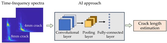
Figure 1.
Schematic of the proposed approach for crack length estimation.
2. FEM Simulation of Fatigue Crack AE
In this section, finite element modeling (FEM) was conducted to study the fatigue-crack-generated AE signals. Commercial finite element package ANSYS 17.0 was used to implement and realize the three-dimensional (3D) FEM model. The dimensions of the FE model are 120 mm × 60 mm × 1 mm. In the simulation, only a half model (Figure 2) was created by applying the symmetric boundary condition to reduce the calculation time. The material properties of aluminum 2024-T3 are given in Table 1.
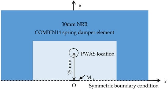
Figure 2.
Schematic of FEM model for the acoustic emission (AE) simulation. (NRB: non-reflective boundary; PWAS: piezoelectric wafer active sensors.)

Table 1.
Material properties of aluminum 2024-T3.
Non-reflective boundaries (NRB) developed in Ref. [35] can eliminate boundary reflections, and thus allow for simulation of guided wave propagation in an infinite medium with small-sized models. 3D structural solid elements (SOLID45) were used to mesh the aluminum plate. COMBIN14 spring-damper elements were used to construct the 30-mm NRB around the model. Figure 2 shows the schematic of FEM model for AE simulation. The mesh size is 1/3 mm for the length and thickness of the model. The dipole moment excitation concept [36] was used to simulate the fatigue crack growth source. In this approach, the AE source due to a fatigue crack growth event was considered as self-equilibrating dipole forces (M11 moment tensor) acting at the crack tip. In the FEM simulation, the M11 dipole excitation was defined using equal and opposite nodal forces. The detailed information can be found in Ref. [36]. The time profile of the excitation was defined as a cosine-bell function with 0.5 µs as the rise time. The parameter summary of the FEM simulation is given in Table 2.
Table 2.
Parameter summary of finite element modeling (FEM) simulation.
First, wavefield analysis was performed to understand the fatigue crack generated AE. The wavefield of surface strain (εxx + εyy) was extracted from the FEM simulations to analyze the wave propagation pattern, as shown in Figure 3. Figure 3a shows the wavefield pattern in a non-cracked specimen and Figure 3b shows the wavefield pattern of an 8-mm crack specimen. It can be found that an additional wave packet was observed due to wave scattering at the crack tip for the case of an 8-mm crack. The AE wave generated at one crack tip travels to the other tip and generates additional propagating waves.
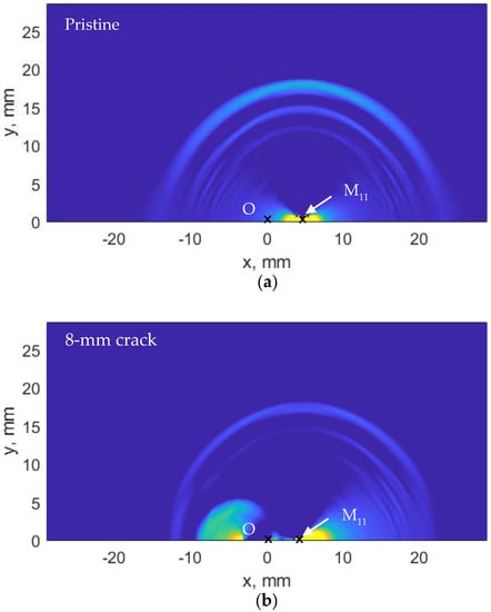
Figure 3.
Wavefield of surface strain (εxx + εyy) due to (a) no crack and (b) 8-mm crack.
Second, nodal strain responses at the location of piezoelectric wafer active sensors (PWAS) sensor were extracted from the FEM simulation. The PWAS location is 25 mm from the origin as shown in Figure 2. To investigate the effect of various crack lengths on AE signals, both nodal response and PWAS response were extracted and calculated for no crack case, 4-mm, 6-mm, and 8-mm crack length, respectively. In this study, the in-plane strain was extracted because the PWAS senses the in-plane strain of the AE signals.
Figure 4 shows the frequency spectra of in-plane strain εxx and εyy of the AE signals at the center node where the PWAS is located, obtained from the FEM simulation. It can be noted that no frequency peaks were observed for the no crack case (Figure 4a). As the crack length increases from 4 mm to 8 mm, the number of frequency peaks increases proportionally. The nodal responses of various crack lengths have specific peaks and valleys in frequency spectra. More specifically, the 4-mm crack (Figure 4b) gives 2 peaks, the 6-mm crack (Figure 4c) has 3 peaks, and the 8-mm crack (Figure 4d) gives 4 peaks in the frequency spectrum. Hence, the frequency of spectrum peaks is directly related to crack length.
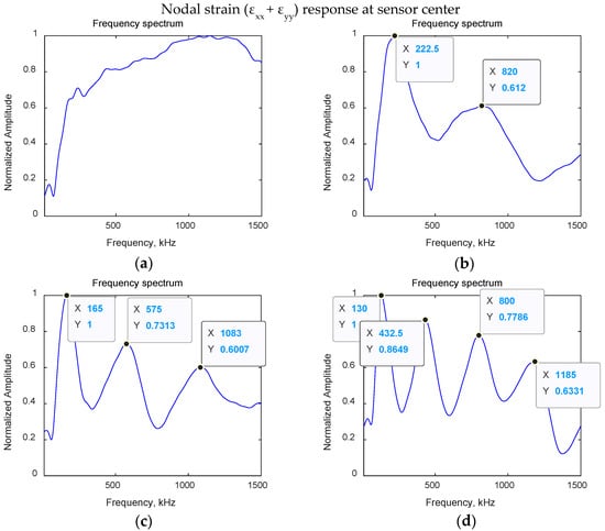
Figure 4.
FFT spectra of nodal strain responses: (a) no crack; (b) with 4-mm crack; (c) with 6-mm crack; and (d) with 8-mm crack. The frequency of spectrum peaks is directly related to crack length.
To compare the FEM simulation result with the experiment, the PWAS response was calculated through the area integration of the in-plane nodal strain within the PWAS region. The PWAS responses were evaluated for the no-crack case, 4-mm crack, 6-mm crack, and 8-mm crack, respectively. The frequency spectra of numerically calculated PWAS responses for all cases are presented in Figure 5. It can be found that the nodal response is modified by the PWAS resonance based on the tuning curve corresponding to the dimensions of the PWAS [37]. The high-frequency response was significantly reduced by the PWAS tuning effect and the number of frequency peaks was also reduced compared to their nodal responses. However, with the change in the crack length, the variation in the frequency spectrum of PWAS response was observed, which means that characteristic frequencies obtained from the AE signal spectrum can be directly related to crack length.
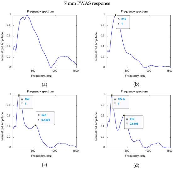
Figure 5.
FFT spectra of 7-mm PWAS responses: (a) No crack; (b) with 4-mm crack; (c) with 6-mm crack; and (d) with 8-mm crack.
3. SIF-Controlled In-Situ Fatigue Experiment
To capture experimental acoustic emission signals, data is gathered from a high-cycle fatigue (HCF) experiment done which held the stress intensity factor (SIF) approximately constant throughout the entirety of the fatigue loading. Given that the stress intensity factor at the tips of a growing crack varies as the crack length progresses, theoretically, one needs to reduce the load as the fatigue crack grows to control the SIF. This SIF-controlled fatigue loading is desired due to the fact that AE signal signatures have been observed to vary with an increase in crack growth rate and SIF. More background details of this SIF-controlled fatigue experimental methodology and its foundation can be found in Ref. [36].
3.1. Experimental Setup
An experimental specimen was designed to collect AE signals during fatigue crack growth in thin metallic plates. A fatigue test coupon of a 1-mm thick aluminum 2024-T3 was cut to a width of 103 mm and a length of 305 mm. The width of the specimen was sufficient to allow a long crack to form. The specimen was fatigue loaded between load limits of 1.38 kN lower bound to 13.85 kN upper bound at a loading frequency of 10 Hz. This loading generated a 4-mm crack along the centerline of the specimen after 322,000 cycles.
After the crack was initiated and grown to 4 mm, the specimen was removed from the MTS machine and AE instrumentation was applied. Two PWAS sensors, two S9225 sensors, and a clay non-reflective boundary were applied to the specimen. The sensors were bonded in a linear configuration at 5 mm and 25 mm from the crack on both sides. The non-reflective boundary was applied to the edges of the specimen to damp out reflecting waves from plate boundaries. The PWAS sensors were bonded using M-Bond AE-15, a two-part epoxy system with a resin and curing agent. This adhesive system was chosen because of its resilience to debonding during excessive fatigue loading. The electromechanical impedance spectrum (EMIS) of the PWAS sensors was measured periodically to ensure no defects or bonding deterioration [37]. The S9225 sensors were bonded using hot glue. Figure 6 shows the setup of this AE test specimen loaded into the MTS machine and ready for AE monitoring.
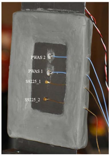
Figure 6.
A 1-mm aluminum 2024 test specimen with AE instrumentation applied: Two PWAS, two S9225, and clay non-reflective boundary.
After AE instrumentation was applied, the test specimen with a 4-mm crack was loaded back into the MTS machine (shown in Figure 6) for further fatigue loading with simultaneous AE monitoring. The system of hardware used in the data acquisition is shown in Figure 7. The Omicron Lab Bode 100 Vector Network Analyzer was used to analyze the EMIS of the bonded PWAS. The PWAS sensors were connected to the MISTRAS AEWinTM computer through an acoustic preamplifier, which is a bandpass filter that filters signals between 30 kHz and 700 kHz. In this experiment, 40 dB of gain was selected on the preamplifier from options of 20 dB, 40 dB, or 60 dB. In the data acquisition software in the AEWinTM system, a sampling frequency of 10 MHz was selected to capture the AE signals from the PWAS. The timing parameters set for the MISTRAS system were peak definition time (PDT) = 200 µs, hit definition time (HDT) = 800 µs, and hit lockout time (HLT) = 1000 µs. Figure 8 also shows the experimental setup and other auxiliary experimental equipment, including the camera and eddy current equipment, which were used to track crack growth continuously. The camera was continuously capturing video of the crack tips with adjacent measurement tape adhered to the test specimen, while an eddy current probe from Eddyfi Technologies® was used periodically to track the growth of the crack.
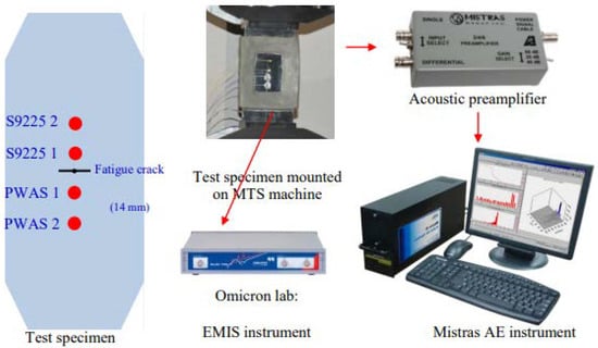
Figure 7.
Experimental setup of the test specimen and data acquisition hardware. (MTS: material testing system; EMIS: electromechanical impedance spectroscopy).
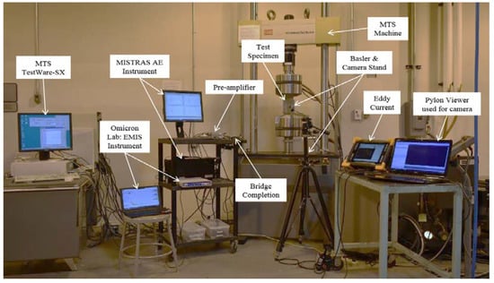
Figure 8.
Experimental setup of fatigue specimen loaded into MTS machine with auxiliary experimental equipment.
3.2. Processing of Experimental Data
With all the AE equipment applied to the specimen, fatigue loading began again at loading bounds of 1.38 kN and 13.85 kN and a loading frequency of 2 Hz. AE events were simultaneously recorded by the AE system shown in Figure 7. Figure 9 shows the overall process flow that the AE data goes through to be analyzed and used in the ensuing novel artificial intelligence system. The process begins with the microcrack growth event which emits strain wave energy that propagates from the tips of the crack (“step 1”). This event is then sensed by the PWAS and picked up within the AEWinTM system (“step 2”). The raw time-domain waveform is stored in the system and then recovered for further processing and analysis (“step 3”). In this processing and analysis of the raw signal, a noise cancellation algorithm is applied to eliminate internal system noise captured with the signal. This cleans up (and removes any noise-related frequencies) the time domain signal as seen in the upper plot of “step 4” in Figure 9. The fast Fourier transform of the signal is then performed to acquire the frequency domain information of the AE wave, as shown in the lower plot of “step 4” in Figure 9. Finally, the Choi–Williams transform (CWT) is performed on the wave (“step 5”). The Choi–Williams distribution (CWD) is a time-frequency transform that is a Cohen class member, which is related to parameters such as the instantaneous median frequency and the instantaneous power (integral over all frequencies at each time) [38,39]. This CWT is a type of wavelet transform that yields an intensity plot that gives information of both the time and frequency domain of the AE wave simultaneously. This CWT result will be the crucial liaison point between the raw signal captured and the application of a convolutional neural network (CNN) for artificial intelligence processing of the AE signals.
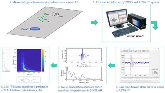
Figure 9.
Flowchart of acoustic emission signal processing from microcrack growth event to the time-frequency intensity plot of Choi–Williams transform.
Continuous fatigue loading may cause disbonding of the PWAS from the specimen. This would result in the capturing of false AE signals. Throughout fatigue loading, the bonding of the PWAS sensor to the specimen was tested using electromechanical impedance spectroscopy (EMIS). The results of this periodic EMIS monitoring are shown in Figure 10, where a good bonding is observed throughout the entirety of the experiment, ensuring no erroneous AE signals.
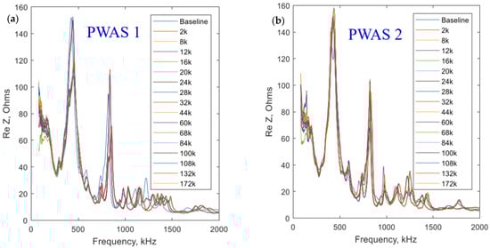
Figure 10.
Periodic EMIS measurement of 172 kcycles of fatigue loading taken at (a) PWAS 1 and (b) PWAS 2.
3.3. Experimental Results
When an acoustic emission is released from the crack, the continuous AE monitoring system senses a hit according to the process depicted in Figure 9. As the crack length grew, the number of acoustic emission hits sensed by the system increased. This is due to favorable crack surfaces for friction engagement, which has been understood to be the main cause of acoustic emissions in a fatigue crack scenario [40]. When the crack was at 8 mm in length, a generous number of signals were captured for analysis.
A sample set of experimental AE signals captured when the crack was 8 mm long is presented in Figure 11. The four signals presented in Figure 11 were representative of the whole set of signals received at this crack length, with similar frequency peaks occurring in all the signals. It is observed from these signals that two common frequency peaks occurred in all of the signals near 123.7 kHz and 410.8 kHz, on average. This trend in the peak-valley pattern, as predicted by the FEM simulations in Section 2, may yield information related to crack length.
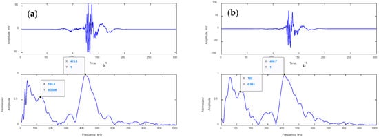
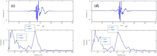
Figure 11.
Experimental acoustic emission signals captured at a crack length of 8 mm: (a) #532, 44-48 kcycles, (b) #652, 44-48 kcycles, (c) #494, 44-48 kcycles, and (d) #446, 44-48 kcycles.
3.4. Comparison to FEM Simulation
As observed in the FEM simulations presented in Section 2, a relationship between the length of a fatigue crack which releases an AE signal and the frequency domain peaks of that signal is predicted. As a primary example of the comparison of the experimental signals to the FEM simulated signals, AE hit #455 from fatigue cycle range 44–48 kcycles, as presented in Figure 12, along with its corresponding CWT intensity plot. This signal is representative of all of the signals in the data set, which show similar characteristics. The CWT is a method of summarizing the time and frequency domain information into an intensity plot, which becomes convenient when building artificial intelligence capabilities for signal analysis. In the CWT of signal #455, we see the frequency peaks at 409.1 kHz and 127.8 kHz manifest in colormap intensity peaks at those frequency values. These frequency peaks match well with the FEM simulations of an 8-mm crack AE signal, which predicts frequency peaks at 127.5 kHz and 410 kHz, as seen in Figure 12.
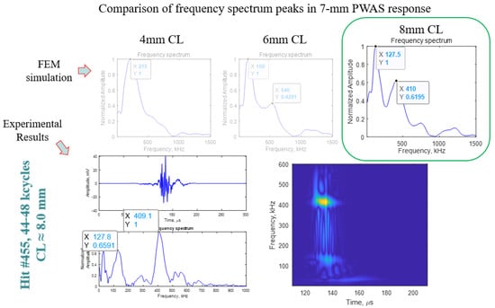
Figure 12.
Time domain, frequency domain, and Choi-William transform of experimental signal #455, 44-48 kcycles (approx. 8 mm) compared to the FEM simulation of an 8-mm crack length AE signal.
These results are very encouraging for both the experimental work done and the parameters involved in creating an accurate finite element model. Ultimately, the good match observed between the FEM simulation and experimental signals mean the FEM results may be utilized to further crack the length prediction efforts of artificial intelligence techniques.
4. Artificial Intelligence Approach for Crack Length Prediction
As the practical application mode of AE-based SHM research is developed, the necessity for applied computing capabilities cultivates. Advanced computing capabilities provide a significant improvement in the development of a comprehensive AE system, where large-scale datasets can be processed efficiently. In the case of the AE approach, an artificial intelligence (AI) system that can serve the role of analyzing the signal waveforms captured to assess details about their origin would prove to be immensely beneficial.
4.1. Introduction to Methodology
In the work presented herein, the AlexNet convolutional neural network (CNN) was used to develop a crack length prediction capability from AE signals. AlexNet is an image classification deep neural network trained on the millions of images contained in ImageNet [41]. The proposed method is not limited to AlexNet; it is simply a generic example. Existing or to-be-developed neural network architectures can also be used to achieve the crack length estimation with system accuracy being the affected result. The general concept of the neural networks follows the standard multilayer perception model which involves appropriately training its neural connections by a backpropagating error and adjusting connection weights following the standard steepest gradient descent [42]. Figure 13 shows the model of a deep neural network, which includes multiple hidden layers of nodes, each connected to the nodes of previous and ensuing layers by weighting factors.
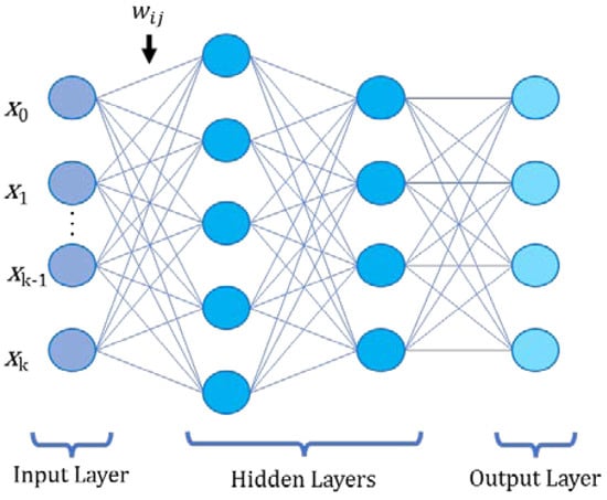
Figure 13.
Schematic of the multilayer perception artificial deep neural network.
For AlexNet, an image recognition convolutional neural network, images of input size 227 × 227 pixels are required. To adopt the experimental AE signals to this criterion, the Choi–Williams transform (CWT) of the waveforms is processed to generate an intensity plot yielding information about the time-domain and frequency-domain of the wave, simultaneously. This intensity plot is then isolated from the legends and associated waveform plots and augmented using MATLAB to conform to the 227 × 227-pixel requirement before being used as input by the AlexNet CNN. A schematic of this process is given in Figure 14.
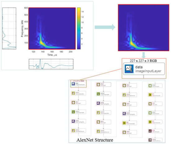
Figure 14.
Choi–Williams transform of the acoustic emission signals is isolated and augmented to fit the 227 × 227-pixel criterion before being entered into the input layer of the AlexNet convolutional neural network architecture.
4.2. Network Training
To build the related CNN for crack length prediction, AE signals were used from the experiment described in Section 3. Here, signals were obtained from the far-field PWAS2 during the experiment when the crack was in the ranges of 3.5–4.5 mm and 7.0–8.0 mm in total length. As previously described in Section 3 and Ref. [22], the fundamental concept is that these AE signals will differ in various characteristics, specifically in the frequency domain. The goal is to build an artificial intelligence system capable of discerning these distinctions and accurately predicting the crack length from the AE signal. Figure 15 shows a schematic of the sensing of the two distinct groups of AE signals used to build an example crack-length estimation CNN. A few examples of the experimental signal CWTs for each of the groups are shown. It is observed from the naked eye that the 7.0–8.0-mm crack length signals have a significant intensity peak near the 410 kHz range, as is also shown in Figure 12, whereas the 3.5–4.5-mm crack length signals do not. Though differentiating other details of the CWT signal subsets may not be easy to the naked eye, training a CNN to do so may yield promising findings.
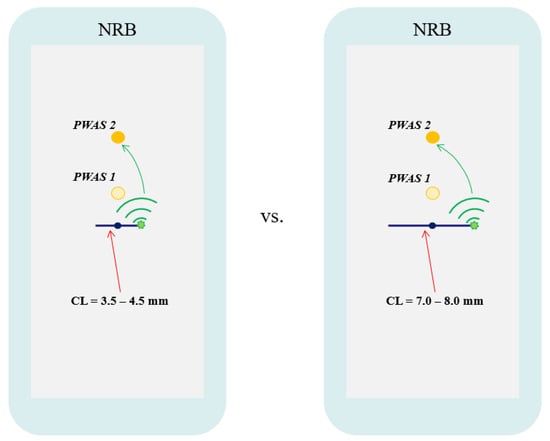
Figure 15.
Schematic of signals from different crack lengths, which will be used to train AlexNet CNN for crack length recognition. (CL: crack length).
The dataset was comprised of a total of 251 CWT figures, 30 of which came from signals of crack lengths 3.5 mm–4.5 mm and 221 of which came from signals of crack lengths 7.0 mm–8.0 mm (as shown in Figure 16). The significant difference in the number of signals from the two groups was a result of more AE signals being captured while the crack was in the 7.0–8.0 mm range due to the more favorable crack surfaces. Due to the small overall dataset, stratified k-fold cross validation was used to partition the data for training and evaluation of the network capability in classifying crack length.
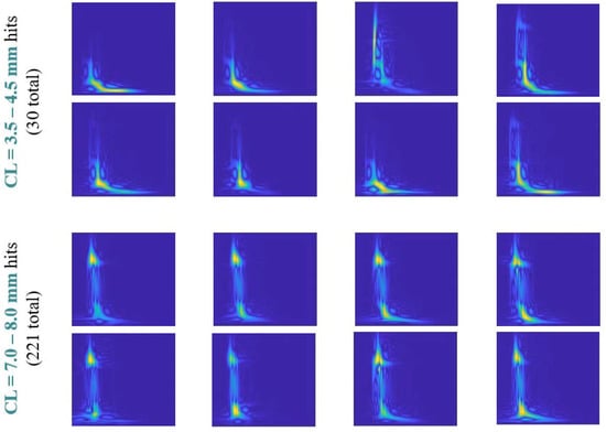
Figure 16.
Example CWT figures for both groups used in crack length recognition AlexNet CNN.
The k value for the stratified k-fold cross validation was selected as 5, which would partition the dataset into 5 equal subsets, each of which has proportional categorical representation from the total dataset. For this network, which was built using the AlexNet convolutional neural network architecture, the optimizer used is the adaptive moment optimization (Adam). Important training options within the Adam optimizer were selected based on experience. The gradient decay factor and squared gradient decay factor were set to 0.9 and 0.999, respectively. The max epochs for each iteration (k = 5) was set to 15 with a validation frequency of 3. The learning rate was an adaptive learning rate in accordance with the Adam optimizer; the initial learning rate was set to a value of 1 × 10⁻⁴. The mini-batch size for the training was 128. The loss function used in this network is the cross-entropy loss.
4.3. Results and Discussion
After each network iteration was sufficiently trained, the network’s performance was tested by assessing its accuracy in predicting the crack length of the validation dataset, which varied with each iteration in accordance with the stratified k-fold cross validation. Each network training iteration involved validating a network accuracy on 20% of the entire dataset (i.e., 50 signals for iteration 1, 2, 4, and 5; 51 signals for iteration 3). The results of the network accuracy following the stratified k-fold cross validation are shown in Table 3. The overall network accuracy, which was computed by taking the average of the k = 5 iterations, was 98.4%.
Table 3.
Network accuracy using stratified k-fold cross validation (k = 5).
From these results, it is observed that a convolutional neural network built using the architecture of AlexNet (although not limited to such architecture) can be utilized to distinguish between various AE experimental fatigue crack signals. The network can be used to build a comprehensive AI system for monitoring fatigue-prone areas in thin metallic sheets. This is accomplished by utilizing the capabilities of this CNN to filter out crack-related vs. noise signals, determine the crack length of a given AE crack-related signal picked up by the monitoring system, and give a prognosis on the remaining useful life of the metallic component.
5. Summary, Conclusions, and Future Work
5.1. Summary
In acoustic emission (AE) structural health monitoring (SHM), post-processing and informative assessment of AE signals is a vitally important piece of the SHM system. In this paper, we investigated the ability to apply artificial intelligence (AI) capabilities to optimize the efficiency of this piece of the SHM system by automating it. FEM analysis was performed to simulate the AE wave propagation from a fatigue crack in metallic plates. A SIF-controlled fatigue experiment was performed to capture AE signals. The resulting experimental signals were compared to the FEM simulations. A fundamental introduction to the principles of applicable AI techniques was shown, and a novel use case of a convolutional neural network (CNN) was presented. The Choi–Williams transforms of AE experimental signals received by a PWAS, which yield an intensity plot containing simultaneous information on both the time domain and frequency domain content of an AE wave, were used as input into the AlexNet CNN in an effort to build a network capable of discerning fatigue crack length.
5.2. Conclusions and Future Work
AE signals captured during a fatigue crack growth experiment were analyzed and found to match closely with the FEM simulations. AE energy generated at one crack tip travels to the other tip and establishes a standing-wave pattern that has a characteristic dominant frequency, which depends on the crack length. A novel approach which utilized the robust image recognition capabilities of the AlexNet convolutional neural network and the Choi–Williams transform of experimental AE signals was presented. This novel AI system proved to be effective at predicting the crack length of an AE signal in a binary scenario at an accuracy of 98.4%. The proposed approach can be used to obtain the crack-length estimation from every AE signal without recourse to the AE-signal history. An invention disclosure [43] covering the developed methodology has been filed.
In future, this concept could be extrapolated to similar applications that go beyond a binary crack length prediction. Regression models could be combined with this more discretized application mode to increase the overall AI capabilities of such a system. As previously mentioned, the approach presented herein is not limited to the AlexNet architecture; further improvements could be explored using other CNN architectures. To expand upon the classification capabilities, further experimentation to capture sufficient datasets in other crack lengths will be valuable to constructing a comprehensive crack monitoring AI system.
Author Contributions
In this article, the formal analysis was done by J.C.G. and H.M. The detailed methodology was provided by J.C.G. and V.G. J.C.G. prepared the original draft; review and editing were done by J.C.G., H.M. and V.G. All authors have read and agreed to the published version of the manuscript.
Funding
This work was supported by the Office of Naval Research (ONR), grant numbers N00014-17-1-2829 and N00014-21-1-2212.
Institutional Review Board Statement
Not applicable.
Informed Consent Statement
Not applicable.
Data Availability Statement
Not applicable.
Conflicts of Interest
The authors declare no conflict of interest.
References
- Catbas, F.N.; Susoy, M.; Frangopol, D.M. Structural health monitoring and reliability estimation: Long span truss bridge application with environmental monitoring data. Eng. Struct. 2008, 30, 2347–2359. [Google Scholar] [CrossRef]
- Mitra, M.; Gopalakrishnan, S. Guided wave based structural health monitoring: A review. Smart Mater. Struct. 2016, 25, 053001. [Google Scholar] [CrossRef]
- Su, Z.; Ye, L.; Lu, Y. Guided Lamb waves for identification of damage in composite structures: A review. J. Sound Vib. 2006, 295, 753–780. [Google Scholar] [CrossRef]
- Mei, H.; Haider, M.F.; Joseph, R.; Migot, A.; Giurgiutiu, V. Recent advances in piezoelectric wafer active sensors for structural health monitoring applications. Sensors 2019, 19, 383. [Google Scholar] [CrossRef] [PubMed] [Green Version]
- Janapati, V.; Kopsaftopoulos, F.; Li, F.; Lee, S.J.; Chang, F.-K. Damage detection sensitivity characterization of acousto-ultrasound-based structural health monitoring techniques. Struct. Health Monit. 2016, 15, 143–161. [Google Scholar] [CrossRef]
- Morton, T.M.; Harrington, R.M.; Bjeletich, J.G. Acoustic emissions of fatigue crack growth. Eng. Fract. Mech. 1973, 5, 691–697. [Google Scholar] [CrossRef]
- Avraham, B.; Fang, D. Study of fatigue crack characteristics by acoustic emission. Eng. Fract. Mech. 1995, 51, 401–416. [Google Scholar]
- Roberts, T.M.; Talebzadeh, M. Acoustic emission monitoring of fatigue crack propagation. J. Constr. Steel Res. 2003, 59, 695–712. [Google Scholar] [CrossRef]
- Lu, Y.; Ye, L.; Su, Z. Crack identification in aluminium plates using Lamb wave signals of a PZT sensor network. Smart Mater. Struct. 2006, 15, 839–849. [Google Scholar] [CrossRef]
- Aggelis, D.G.; Kordatos, E.Z.; Metikas, T.E. Acoustic emission for fatigue damage characterization in metal plates. Mech. Res. Commun. 2011, 38, 106–110. [Google Scholar] [CrossRef]
- Chai, M.; Zhang, J.; Zhang, Z.; Duan, Q.; Cheng, G. Acoustic emission studies for characterization of fatigue crack growth in 316LN stainless steel and welds. Appl. Acoust. 2017, 126, 101–113. [Google Scholar] [CrossRef]
- Haider, M.F.; Giurgiutiu, V. Theoretical and numerical analysis of acoustic emission guided waves released during crack propagation. J. Intell. Mater. Syst. Struct. 2016, 30, 1318–1338. [Google Scholar] [CrossRef]
- Barat, V.; Terentyev, D.; Bardakov, V.; Elizarov, S. Analytical Modeling of Acoustic Emission Signals in Thin-Walled Objects. Appl. Sci. 2020, 10, 279. [Google Scholar] [CrossRef] [Green Version]
- Pascoe, J.A.; Zarouchas, D.S.; Alderliesten, R.C.; Benedictus, R. Using acoustic emission to understand fatigue crack growth within a single load cycle. Eng. Fract. Mech. 2018, 194, 281–300. [Google Scholar] [CrossRef] [Green Version]
- Zheng, H.; Sladek, J.; Sladek, V.; Wang, S.K.; Wen, P.H. Hybrid meshless/displacement discontinuity method for FGM Reissner’s plate with cracks. Appl. Math. Model. 2021, 90, 1226–1244. [Google Scholar] [CrossRef]
- Zheng, H.; Yang, Z.; Zhang, C.; Tyrer, M. A local radial basis function collocation method for band structure computation of phononic crystals with scatterers of arbitrary geometry. Appl. Math. Model. 2018, 60, 447–459. [Google Scholar] [CrossRef]
- Ali, H.Q.; Tabrizi, I.E.; Khan, R.M.A.; Tufani, A.; Yildiz, M. Microscopic analysis of failure in woven carbon fabric laminates coupled with digital image correlation and acoustic emission. Compos. Struct. 2019, 230, 111515. [Google Scholar] [CrossRef]
- Beheshtizadeh, N.; Mostafapour, A. Processing of acoustic signals via wavelet & Choi—Williams analysis in three-point bending load of carbon/epoxy and glass/epoxy composites. Ultrasonics 2017, 79, 1–8. [Google Scholar]
- Djabali, A.; Toubal, L.; Zitoune, R.; Rechak, S. Fatigue damage evolution in thick composite laminates: Combination of X-ray tomography, acoustic emission and digital image correlation. Compos. Sci. Technol. 2019, 183, 107815. [Google Scholar] [CrossRef]
- Roundi, W.; Mahi, A.E.; Gharad, A.E.; Rebiere, J.-L. Acoustic emission monitoring of damage progression in Glass/Epoxy composites during static and fatigue tensile tests. Appl. Acoust. 2018, 132, 124–134. [Google Scholar] [CrossRef]
- Saeedifar, M.; Mansvelder, J.; Mohammadi, R.; Zarouchas, D. Using passive and active acoustic methods for impact damage assessment of composite structures. Compos. Struct. 2019, 226, 111252. [Google Scholar] [CrossRef] [Green Version]
- Joseph, R.; Mei, H.; Migot, A.; Giurgiutiu, V. Crack-Length Estimation for Structural Health Monitoring Using the High-Frequency Resonances Excited by the Energy Release during Fatigue-Crack Growth. Sensors 2021, 21, 4221. [Google Scholar] [CrossRef] [PubMed]
- Tang, J.; Soua, S.; Mares, C.; Gan, T.-H. A Pattern Recognition Approach to Acoustic Emission Data Originating from Fatigue of Wind Turbine Blades. Sensors 2017, 17, 2507. [Google Scholar] [CrossRef] [PubMed] [Green Version]
- Xu, D.; Liu, P.F.; Li, J.G.; Chen, Z.P. Damage mode identification of adhesive composite joints under hygrothermal environment using acoustic emission and machine learning. Compos. Struct. 2019, 211, 351–363. [Google Scholar] [CrossRef]
- Ren, Y.; Qiu, L.; Yuan, S.; Fang, F. Multi-damage imaging of composite structures under environmental and operational conditions using guided wave and Gaussian mixture model. Smart Mater. Struct. 2019, 28, 115017. [Google Scholar] [CrossRef]
- Xu, J.; Wang, W.; Han, Q.; Liu, X. Damage pattern recognition and damage evolution analysis of unidirectional CFRP tendons under tensile loading using acoustic emission technology. Compos. Struct. 2020, 238, 111948. [Google Scholar] [CrossRef]
- Ramasso, E.; Butaud, P.; Jeannin, T.; Sarasini, F.; Placet, V.; Godin, N.; Tirillo, J.; Gabrion, X. Learning the representation of raw acoustic emission signals by direct generative modelling and its use in chronology-based clusters identification. Eng. Appl. Artif. Intell. 2020, 90, 103478. [Google Scholar] [CrossRef]
- Yuen, K.; Lam, H. On the complexity of artificial neural networks for smart structures monitoring. Eng. Struct. 2006, 28, 977–984. [Google Scholar] [CrossRef]
- Mehrjoo, M.; Khaji, N.; Moharrami, H.; Behreininejad, A. Damage detection of truss bridge joints using Artificial Neural Networks. Expert Syst. Appl. 2008, 35, 1122–1131. [Google Scholar] [CrossRef]
- Tao, C.; Zhang, C.; Ji, H.; Qiu, J. Fatigue damage characterization for composite laminates using deep learning and laser ultrasonic. Compos. Part B Eng. 2021, 216, 108816. [Google Scholar] [CrossRef]
- Nasiri, S.; Khosravani, M.R. Machine learning in predicting mechanical behavior of additively manufactured parts. J. Mater. Res. Technol. 2021, 14, 1137–1153. [Google Scholar] [CrossRef]
- Wiangkham, A.; Ariyarit, A.; Aengchuan, P. Prediction of the mixed mode I/II fracture toughness of PMMA by an artificial intelligence approach. Theor. Appl. Fract. Mech. 2021, 112, 102910. [Google Scholar] [CrossRef]
- Han, X.; Xiao, Q.; Cui, K.; Hu, X.; Chen, Q.; Li, C.; Qiu, Z. Predicting the fracture behavior of concrete using artificial intelligence approaches and closed-form solution. Theor. Appl. Fract. Mech. 2021, 112, 102892. [Google Scholar] [CrossRef]
- Khosravani, M.R.; Nasiri, S.; Weinberg, K. Prediction of fracture in sandwich-structured composite joints using case-based reasoning approach. Procedia Struct. Integr. 2018, 13, 168–173. [Google Scholar] [CrossRef]
- Shen, Y.; Giurgiutiu, V. Effective non-reflective boundary for Lamb waves: Theory, finite element implementation, and applications. Wave Motion 2015, 58, 22–41. [Google Scholar] [CrossRef] [Green Version]
- Joseph, R. Acoustic Emission and Guided Wave Modeling and Experiments for Structural Health Monitoring and Non-Destructive Evaluation. Ph.D. Thesis, University of South Carolina, Columbia, SC, USA, 2020. [Google Scholar]
- Giurgiutiu, V. Structural Health Monitoring with Piezoelectric Wafer Active Sensors, 2nd ed.; Elsevier Academic Press: Waltham, MA, USA, 2014; ISBN 978-0-12-418691-0. [Google Scholar]
- Choi, H.-I.; Williams, W.J. Improved Time-Frequency Representation of Multicomponent Signals Using Exponential Kernels. IEEE Trans. Acoust. Speech Signal Process. 1989, 37, 862–871. [Google Scholar] [CrossRef]
- Pereira, G.R.; de Oliveira, L.F.; Nadal, J. Reducing cross terms effects in the Choi–Williams transform of mioelectric signals. Comput. Methods Programs Biomed. 2013, 111, 685–692. [Google Scholar] [CrossRef] [Green Version]
- Joseph, R.P.; Giurgiutiu, V. Acoustic emission (AE) fatigue-crack source modeling and simulation using moment tensor concept. In Proceedings of the SPIE Smart Structures + Nondestructive Evaluation, Online, 27 April–9 May 2020; Volume 11379. [Google Scholar]
- Krizhevsky, A.; Sutskever, I.; Hinton, G.E. ImageNet Classification with Deep Convolutional Neural Networks. Adv. Neural Inf. Process. Syst. 2012, 25, 1097–1105. [Google Scholar] [CrossRef]
- Farrar, D.R.; Worden, K. Structural Health Monitoring: A Machine Learning Perspective; John Wiley & Sons, Ltd.: West Sussex, UK, 2013. [Google Scholar]
- Giurgiutiu, V.; Mei, H.; Garrett, J.; Cardillo, K. AI Method-Apparatus for Extracting Crack-Length from High-Frequency AE Signals; USC-IPMO, Disclosure ID No. 1536. May 2021. [Google Scholar]
Publisher’s Note: MDPI stays neutral with regard to jurisdictional claims in published maps and institutional affiliations. |
© 2022 by the authors. Licensee MDPI, Basel, Switzerland. This article is an open access article distributed under the terms and conditions of the Creative Commons Attribution (CC BY) license (https://creativecommons.org/licenses/by/4.0/).