Abstract
Deep Neural Networks (DNNs) have shown superior accuracy at the expense of high memory and computation requirements. Optimizing DNN models regarding energy and hardware resource requirements is extremely important for applications with resource-constrained embedded environments. Although using binary neural networks (BNNs), one of the recent promising approaches, significantly reduces the design’s complexity, accuracy degradation is inevitable when reducing the precision of parameters and output activations. To balance between implementation cost and accuracy, in addition to proposing specialized hardware accelerators for corresponding specific network models, most recent software binary neural networks have been optimized based on generalized metrics, such as FLOPs or MAC operation requirements. However, with the wide range of hardware available today, independently evaluating software network structures is not good enough to determine the final network model for typical devices. In this paper, an architecture search algorithm based on estimating the hardware performance at the design time is proposed to achieve the best binary neural network models for hardware implementation on target platforms. With the XNOR-net used as a base architecture and target platforms, including Field Programmable Gate Array (FPGA), Graphic Processing Unit (GPU), and Resistive Random Access Memory (RRAM), the proposed algorithm shows its efficiency by giving more accurate estimation for the hardware performance at the design time than FLOPs or MAC operations.
1. Introduction
In recent years, deep learning has demonstrated incredible performance in diverse research areas with different tasks, such as classification and detection [1,2]. To expand the scope of application with enormous datasets and stricter requirements, deep neural networks have been deployed with deeper and bigger model sizes, leading to more computational, memory resources, and power consumption. Hence, optimizing them in terms of memory and computations is an active research area [3,4,5,6,7,8,9,10]. Researchers have shown various methods that are effective in optimizing the deep learning models. Pruning [3,4,5] removes unnecessary weights from the neural network. Quantization [5,6,7] reduces the bit-widths of the weights and activations. These methods help produce lighter and faster neural networks. One of the most aggressive forms of quantization is used in Binarized Neural Networks [10] and XNOR-Nets [9]. In these methods, the weights and activations are both reduced to 1-bit precision. Since the network only uses 1-bit weight and activations, computing BNNs can be extremely fast and light-weight. However, the massive reduction in the network results in substantial accuracy degradation. Therefore, generating a binary neural network model that can be implemented with the best power and resource efficiency while maintaining reasonable accuracy has recently been one of the critical research objectives.
To take full advantages of the BNN and limit the impact on accuracy, from the training solution of Courbariaux et al. in 2016 [10], many approaches have been proposed for training strategies and hardware implementation. For the training process, a low learning rate, PReLu, and new regularization term are newly proposed ideas in [11] to improve accuracy and training stability. Approximating the full-precision weight with a linear combination and employing multiple binary activations are other techniques applied to increase accuracy [12]. In addition, new BNN architectures were proposed with higher accuracy. For example, the authors in [13] proposed a new neural structure called ReActNet, which can improve accuracy without any additional computational cost through generalizing the traditional Sign, PReLU functions, and new distribution loss. Moreover, a new approach to compensate for accuracy degradation is introduced in [14] with a rotated binary neural network (RBNN), which considers the angle alignment between the full-precision weight vector and its binarized version. In optimizing hardware implementation, processing in-memory computing and accelerators on FPGA are popular directions used to deploy the BNN architecture. In particular, XNOR logic for multiplication, popcount for binary accumulation, threshold comparison for batchnorm operation, and OR logic for max-pooling are well-known methods applied for the digital circuit on ASIC or FPGA [15,16,17,18]. Meanwhile, regarding memory computing, a series of papers were published and proved their ability in enhancing power and resource efficiency [19,20,21,22].
In general, in addition to proposing specialized accelerators for specific software neural network models to achieve optimization goals, at the software level, most researchers have tried to minimize computational cost and the number of parameters based on generalized metrics, such as MAC operations. At the coarse-tuning stage, this direction efficiently reduces evaluation time and gives us a quick overview of hardware overhead when implementing the neural network. Nevertheless, at the fine-tuning stage for specific target hardware, this information is not enough or can even make a wrong decision when choosing the relevant model to implement because of their distinctive properties. More specifically, the same network design may yield different costs in different hardware platforms. In addition, if a BNN model is implemented in a GPU platform or custom hardware platform, such as FPGA or ASIC implementations, the optimal model constructions can be significantly different because the cost hardware platforms can provide various optimized hardware operations. Therefore, although measuring hardware performance at design time is challenging, it should be an indispensable part to find out the best neural network model for corresponding hardware platforms.
In this paper, to design a hardware platform-aware optimal BNN, we propose a new framework that can analyze and explore the ultimate software model based on the estimation of the hardware performance with optimal effort and an architecture search for the training period. In particular, firstly, the advantages of BNNs, such as low computational cost, low memory area, are utilized to construct hardware cost estimation charts that can provide more exact information about hardware implementation for the evaluated models. Secondly, we present a neural network search algorithm called Deepbit, which can explore optimal BNN models for target hardware platforms by using the binary search method and hardware cost estimation charts. More specifically, our method is performed over three steps:
- Pre-Training: Before training, we develop cost estimation charts. The cost estimation charts are developed by deploying various models on the target hardware and calculating their actual costs.
- Training: We propose the Deepbit method, which searches over a large hyperspace and outputs a series of efficient BNN models with variable depths.
- Post-Training: Finally, we use the cost estimation charts to predict the performance of our networks on actual hardware. Based on the predictions, we choose the most efficient network. In the scope of this paper, FPGA, GPU, and RRAM are target hardware platforms, while the MNIST dataset is used for training to demonstrate the effectiveness of our method.
Although the proposed method increases the computation at the training time, it can provide a more accurate DNN model architectural search metric than independent software evaluation methods. Since the training is performed on GPU servers that are resourceful environments in terms of computing performance, power, and temperature, it is much favorable to increase the computation at the training time if it results in an efficient neural network for the targeted hardware.
The rest of the paper is organized as follows. Section 2 introduces a common background related to BNN and prior work related to the proposed solution. Section 3 explains basic design strategies used for the network to reduce the search space. The proposed method to develop the cost estimation charts and the architecture search is presented in Section 4. Section 5 shows the experimental results and discussions. Finally, the paper is concluded in the last section.
2. Background and Related Work
2.1. Related Work
The previous work related to optimizing BNNs for hardware implementation is divided into some categories. In the first category, some publications have focused on proposing hardware techniques to reduce hardware costs for any available software neural networks. For example, in [15,16], based on the advantages of the binary characteristic, the authors proposed some techniques, such as replacing max-pooling with OR operation, using a threshold for batch normalization, Matrix-Vector–Threshold Unit (MVTU) to reduce hardware overhead, and power consumption on binary convolution layers. The authors in [18,23] proposed using the difference between the binary weight array to reduce computation effort on both binary convolution and fully connected layers. The popcount compression and Xnor-based binary MAC were applied in [17] to reduce hardware resources on the BNN model independently. For in-memory computing, in [20], the authors proposed mixed-signal in-memory computing (IMC) SRAM macro that can compute ternary-XNOR-and-accumulate (XAC) operations in binary neural networks without row-by-row data access. The proposed method gave better energy efficiency and energy-delay product than conventional digital hardware. Moreover, RRAM was also utilized in the paper [19] with a synaptic architecture (XNOR-RRAM) that can implement equivalent XNOR and bit-counting operations. Based on these methods, BNNs can be effectively optimized by evaluating the direct feedback from the hardware implementation results. Other well-known methods used for hardware optimization can be found in [24,25,26,27,28,29,30,31,32]. All compatible hardware techniques are flexibly used to optimize the design without impacts on software functions of BNNs. However, only focusing on the hardware implementation would not be a comprehensive optimization method when the software stage can also potentially combine with the hardware implementation to provide better results for any specific hardware platform with distinctive advantages.
The second category is software optimization. Most methods in this category independently optimize the software models based on generalized metrics, such as accuracy, FLOPS, and MAC operations. For example, in [33], to estimate the performance of the network, the author proposed an architecture neural network search using reinforcement learning to explore optimal neural network models based on accuracy and training time. Transferable Architectures is proposed in [34] to reduce the search space for larges datasets based on the training result from smaller ones. To evaluate the effectiveness of the solution, FLOPs and accuracy criteria are also used for comparison. Moreover, some well-known techniques, such as skip-connection, depth-wise separable convolution, Squeeze and Excitation, inverted-bottleneck, and leaky-relu, were proposed for recent DNN models and have given considerable high-accuracy reductions related to the number of parameters or MAC operations. However, the network with minimal FLOPs [35] or MAC operations may not reflect the actual hardware overhead or other critical costs of specific hardware platforms.
The third category is optimizing the software models based on feedback from hardware implementation results. The authors in [36,37,38,39] consider the inference performance of the DNN models. However, they only target one type of hardware platform—ARM architecture for mobile devices. Recent gradient-based methods [37,40,41] use direct metrics for mobile CPUs. In particular, in [37], the authors mainly focused on latency to evaluate the efficiency of the optimal neural network when implementing it in mobile platforms. Moreover, Ref. [42] created a hardware simulator that generates latency and energy for the Reinforcement Learning process to automatically determine the quantization policy for each layer in specific neural networks. An automated mobile neural architecture search was proposed in [43], in which a model latency, which measures the actual latency on mobile devices, is included in the main objective. Hence, the search can identify a model that achieves a desirable trade-off between accuracy and latency. However, there is a variety of smart devices equipped with different types of hardware, such as GPU, CPU, FPGA, ReRam, DSP, and various AI accelerators, such as Google TPU [44], Intel Movidius [45], and Nvidia Jetson [46]. All of these devices have different hardware designs and operational characteristics. This causes the same network architecture to perform with different operational characteristics (latency, throughput, power consumption, heat, etc.) in each of them. Therefore, it is also not optimal to recursively run a network architecture on the target hardware to include the hardware performance in the design loop. Considering these limitations of the existing systems, we propose a new approach in this paper. Cost estimation charts are prepared based on the proposed method and the type of hardware platforms before training and optimizing the target network architecture. This gives a much more accurate hardware performance estimate than FLOPs or MAC operations.
In terms of the previous works related to searching neural networks for specific target hardware platforms with a fixed configuration, as introduced in [47], the goal of this approach is to find the best architecture in terms of accuracy and hardware efficiency for one single target hardware. If new hardware or requirements have to be used for the searching process, the entire process must be returned with the new setting and constraints. Because, at each searching time, the architecture search can solely focus on several specific hardware requirements. In this approach, two options are commonly selected: provide a new configuration by updating the search strategy or search space.
For the updating strategy [36,37,48,49,50,51,52,53], in addition to optimizing accuracy, a component used to measure hardware cost metrics updates the target constraints (latency, power consumption, hardware resources). It then provides the results to guide the searching process toward finding the desirable model for the reconfiguration. Most researchers use this direction due to the enormous computational and time reduction. However, measuring each operation on a real hardware platform still cannot show the full effects of constraints on a whole model. Furthermore, each target configuration can have different effects when measured on a whole model, causing the searching process not to obtain the best model for hardware implementation.
For updating space [54,55,56,57,58], this is the direction that we perform in this paper. In particular, prior work measured the operators’ performance and set some rules to narrow the searching space based on the initial conditions. Next, the training process maximizes the accuracy under constrained searching space and without cooperation with other hardware metrics. This method can reduce the training time and be more effortless in performing the searching process because the training process is like conventional searching direction and independent of the hardware requirement. However, measuring the performance of each operation may not show the correct effects on the entire searching model, which may cause the searching space to be wrong. In addition, the search strategy may not find the most desirable model during the searching process when the training model does not depend on any hardware performance feedback. In our proposed method, because the model is a binary neural network, it is easier to implement the models on target hardware than full prevision neural networks. In doing so, hardware cost estimation charts can measure the effects of initial conditions more precisely than measuring each operation’s performance. Because target conditions from hardware evaluation all need to have the minimum number of channels on each layer (as explained in Section 4.2), after narrowing the searching process, our method proposed minimizing the number of channels on each layer while trying to meet the threshold accuracy. Moreover, at the end of the searching process, the final optimal model is selected by evaluating the hardware cost based on the hardware cost estimation charts. Consequently, hardware estimation is included in the searching process instead of training without hardware constraints, as in prior work.
2.2. Binarized Neural Networks (BNNs)
Over the recent years, Binarized Neural Networks (BNNs) have been highly favored by researchers due to their hardware-friendly characteristics. With only two states for their weights and activations, BNNs significantly boost the target hardware by reducing their memory consumption and computation effort. In particular, as in [9], the authors introduced an Xnor-Nets, which quantizes the weights and activations to +1 or −1 in the following equation:
where is the output of the function after binarizing. Based on this characteristic, in BNNs, the multiplication operations of both convolution and fully connected layers can be simplified to simple XNOR operations, while the accumulation operation is replaced by the popcount operation without accuracy degradation, as shown in Figure 1. On the other hand, with only one-bit representation, memory used for parameters and output activation storage reduces by almost 32× compared to 32 bit-full precision weights and activation. Consequently, power consumption for memory access considerably reduces with BNN models rather than conventional convolution or fully connected layers. These mentioned advantages from BNNs are the reason leading to an increase in preference of researchers towards BNNs with resource-constrained hardware.
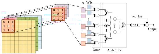
Figure 1.
Xnor operation and accumulation on a convolution layer.
In the scope of this paper, the deployment of BNNs in resource-constrained hardware is studied. More specifically, the implementation for training our BNNs has followed the method in [10], where the input pixels of the first layer are not binarized. Accordingly, an architecture search algorithm that can estimate the hardware performance at the design time is performed to explore BNNs explicitly optimized for the target hardware. The design strategies for our BNNs are explained in detail in the following sections. Moreover, the architecture search algorithm and hardware cost estimation at the design time is also described.
3. Basic Design Strategies
The DNN model architectural search is computationally costly with an infinitely large search space. Thus, this paper defines some basic design principles that can narrow down the search space and considerably reduce the computational complexity of the architectural search. Typically, the Binarized Neural Network is used for the experiments based on the implementation in [9] with the MNIST dataset. That means all the weights and activations are binarized except for the input pixels of the first convolution layer. In addition, the proposed approach manipulates only the convolution layers to find efficient network architectures while keeping one fully connected layer at the end of all experimental neural networks for classification.
In this paper, the searching space only focuses on standard convolution layers, with a 3 × 3 kernel size, which is sufficient to provide high accuracy for the MNIST dataset. Meanwhile, point-wise, depth-wise convolution, residual neural network, and bigger than 3 × 3 kernel size are out of searching space to avoid high memory access and reduce the complexity as well as the searching time for our searching algorithm. Regarding the activation function, batch normalization and the Tanh activation function are applied for each convolution layer.
On the other hand, the well-known pooling technique is also added to the experimental neural networks as a fundamental design strategy to reduce the computational cost further. Using the mentioned kernel size and activation functions, in Table 1, a few binary neural network models, including three convolution layers and one fully connected layer at the end, are prepared with a different number of added pooling layers and kept the same for the rest to estimate the effect of the pooling method based on the number of MAC operations and the accuracy.

Table 1.
Effect of adding pooling layers.
Accordingly, adding up to two pooling layers for the last two convolutions has a minor effect on accuracy with 0.1% degradation and a substantial decrease in MAC operations with 38%. Meanwhile, adding one pooling layer gives a trivial reduction in the number of MAC operations. Hence, using two pooling layers is selected for the architecture search algorithm in this paper. Moreover, the type of pooling layer is also considered for searching space. As shown in Table 2, an accuracy comparison between a model using only max-pooling layers and average pooling layers is described. In particular, the number of convolution layers is still 3, accompanying the mentioned activation functions, and a fully connected layer is attached at the end of these models. The number of channels on each layer is the same and equal to 32. The two last convolution layers are used to add pooling layers for both average pooling and max pooling. Based on the result, max-pooling would be used for the scope of the evaluation with a better-produced accuracy rather than average pooling. Finally, based on our design considerations, the base module for each layer is shown in Figure 2.
Table 2.
Max pooling vs. Average pooling.
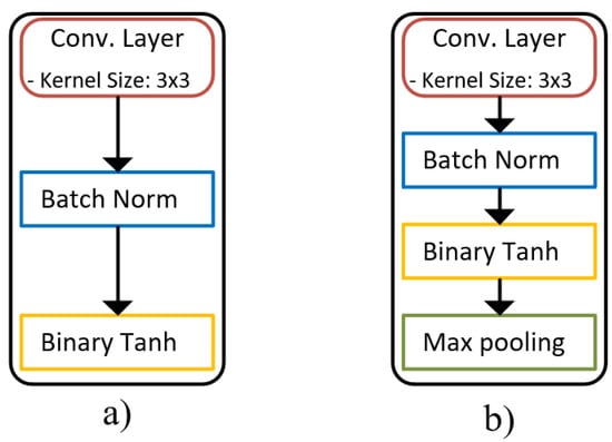
Figure 2.
The building module for a network architecture: (a) layer module for our network architecture; (b) layer module for our network architecture with Max pooling.
In summary, only the number of layers and channels are adjusted to find the optimal architecture. It should be noted that the strictness of design strategies should depend on the training resources. Based on our design strategy, we try to optimize six models in terms of channels per layer, each with the depth ranging from 3 to 8. Given higher training resources, we can obtain 12 models, 6 with max-pooling in the last 2 layers and 6 with average pooling in the last 2 layers.
4. Proposed Architecture Search Solution
To determine the ultimate optimal BNN model for hardware implementation, as mentioned in the previous section, this work proposes the architecture search method that can analyze and explore the ultimate software model based on a combination between the training and hardware cost estimation process. Figure 3 shows a generic block diagram of the architecture searching method. In particular, with the basic design strategies, a series of BNN models are implemented on the target hardware platform, and then hardware estimation charts, including the number of critical resources used for these models, is constructed.
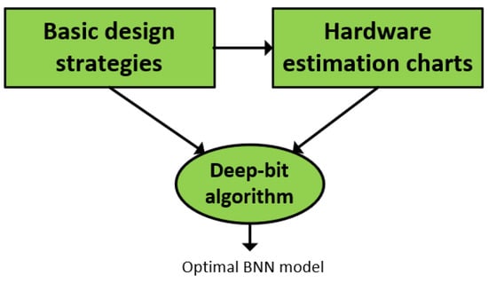
Figure 3.
A generic block diagram for the architecture searching process.
Moreover, a searching algorithm called Deepbit is also performed to explore the final optimal BNN model, with inputs being accuracy threshold, hardware estimation charts, and basic design strategies. The details of hardware cost estimation and Deepbit algorithm are explained as follows.
4.1. Hardware Cost Estimation
Cost estimation charts are considered Look Up Tables used to evaluate the hardware cost among neural network models during the searching process. Depending on the type of hardware platforms, critical resources would be different. In particular, regarding hardware platforms, in this paper, FPGA devices with BNN streaming architectures, RRAM with IR drop and sneak path effects [59,60] and GPU are targeted to find the corresponding optimal software model.
In terms of FPGAs, a BNN streaming architecture is fully implemented to evaluate the method. The architecture is a multi-layer architecture where a separate hardware block accelerates each layer of the BNN. The design is achieved at the coarse-grained pipeline level by dividing an inference workload into a layer granularity. The number of pipeline stages is equal to the number of layers. In Figure 4, a general block diagram of the accelerator is described. For the layer level, pipelining accompanied by the parallelism technique is effectively applied. Typically, light-weight line buffers are responsible for data conveyed among layers, while XNOR-popcount handles all multiplications and accumulation with specific parallel levels. On the other hand, because binary weight spends much smaller memory than full precision weight, all parameters are stored by FPGA registers. The design with this approach eliminates power consumption, data transmission latency from external memory, and on-chip memory to the design. Moreover, because the output of the batchnorm operation is binarized before delivering to the next layers, this operation is replaced by a comparison with a threshold, accompanied by a XNOR operation as in Equation (2), in which is a small number to avoid a round-off problem, and are the mean and variance of the train data batch, and and are constants learned from the training process.
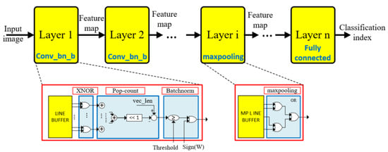
Figure 4.
Binarized Neural Network hardware architecture on FPGA.
The max-pooling is implemented by using the OR operation [16] to OR 4 input values instead of finding the maximum value because the output of this operation is also binarized.
For RRAM devices, we do not own a physical device. Therefore, we create an RRAM simulator in PyTorch, in which the error including on the RRAM device is also replicated. More specifically, to emulate the accuracy deviation, the trained models are injected with a certain amount of error into every output channel of each layer. The amount of errors is approximated based on IR drop and sneak path effects [59,60] to satisfy the accuracy deviation, as mentioned in [59], in which the array size is the number of channels or width of a layer. Accordingly, if the number of channels increases, the accuracy deviation increases. Based on the software simulator, we explore the BNN model, which would perform optimally on an actual RRAM device.
The size of a chart depends on the search scope (the range of network width and depth), hardware implementation cost, and implementation time. More data would give better estimation results and consequently provide better neural network models for hardware implementation. However, in this paper, to explore a particular maximum number of layers for the searching process, we evaluate accuracy for a list of models with appropriate steps for increasing the number of layers and channels in constructing hardware estimation charts for GPU. In particular, depending on the dataset size, the steps for increasing the number of layers (2 for MNIST) and for increasing the number of channels (10 for MNIST) are defined. Then, the training is performed for all models with the corresponding number of layers and channels, which can be obtained by adding up the steps. According to the results, we can see the correlation between accuracy and the number of channels and layers. For example, according to Table 3 (GPU estimation charts for the MNIST dataset), the threshold accuracy can be obtained for 3 to 8 layers with a number of channels under 50 for the MNIST dataset. Meanwhile, with more than 8 layers, the accuracy tends to be saturated.
Table 3.
GPU accuracy estimation charts.
To make the cost estimation charts’ creation more understandable, an example used for the paper’s experiments is provided. More specifically, the range for network width is defined between 5 and 50, with an interval of 5, while the network depth is defined between 3 and 10, as the following.
Based on these ranges, L× C BNN models given by the Cartesian product of set L and set C, as shown in Table 4, are prepared for the hardware evaluation and training process, in which L is the number of convolution layers and C is the number of channels in each layer. All these models are initialized with random weights and then deployed on target hardware platforms to obtain actual hardware costs. Depending on the target hardware platform, the cost metrics can be from different criteria, but all represent the most critical resource of the corresponding target hardware. For example, in RRAM, the RRAM accuracy is one of the cost metrics. However, in FPGAs, power consumption, Look Up Tables (LUTs), and flip-flops are cost metrics. Based on these costs, the hardware cost estimation is performed during the searching time to find the best software model for each corresponding targeted accuracy. This direction saves us from rigorous hardware testing after training optimal models. It is noticeable that the cost estimation charts need to be developed only once for a specific hardware platform and can be referred to in the future by other researchers. The only condition is that the search space for the architectural search should be a subset of the search space of the cost estimation charts. Table 4 and Figure 5 are examples of such charts for BNN models’ power consumption and hardware resources. Firstly, Table 4 describes the power consumption of all models we can have based on the range of width and depth after implementing them on a particular FPGA platform. Each pair of width and depth corresponds to a model. The structure of each layer in a model follows the design strategy introduced in Section 3. Secondly, Figure 5 is another representation of hardware estimation charts, in which the number of layers varies in the range from 3 to 4, and the number of channels varies from 5 to 30 channels.
Table 4.
Cost estimation charts for power consumption.
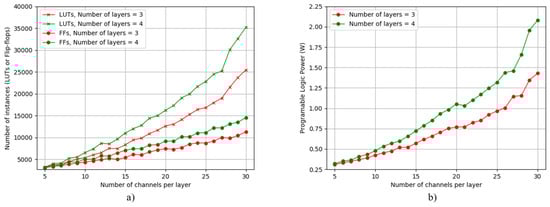
Figure 5.
The hardware and power cost estimation for a list of BNN models with different L and C values on FPGA: (a) hardware resources for BNN models with different L and C values on FPGA; (b) power consumption for BNN models with different L and C values on FPGA.
4.2. Architectural Search via Deepbit Method
Deepbit algorithm is the most crucial part of the proposed solution, which is responsible for training and hardware evaluation to explore the optimal model for a specific hardware platform. In particular, the training process is performed first for a series of BNN models to reduce the searching scope. Next, hardware cost for output BNN models is estimated according to the hardware cost estimation charts. Finally, the ultimate optimal BNN model is determined based on hardware cost comparison among BNN models. The detail of an example used for our experiments is described with the following input:
- The set L defines the range for the depth (the number of convolution layers) of the BNN model. In our experiments:
- The maximum number of uniform channels per layer. In our experiments, we set this value at 50.
- The threshold for an acceptable model. In most cases, the threshold is the minimum acceptable accuracy.
As introduced in the previous section, the target platforms of this paper are FPGA devices with streaming BNN architecture, RRAM devices with the influence of the IR drop and sneak path [59,60] and GPU. For FPGA devices, because streaming BNN architectures are fully implemented on FPGA, with a certain number of layers, an increase in the number of channels on each layer directly increases the hardware resources and power consumption, as shown in Figure 5. Hence, minimizing the number of channels on each layer becomes the target of the Deepbit algorithm during the searching process. Similar to FPGA devices with streaming BNN architecture, RRAM devices affected by IR drop and sneak path also consider minimizing the number of channels on each layer an essential factor needed to perform. In particular, as shown in Figure 6, when increasing the number of channels into each layer, the accuracy is affected more severely, and the accuracy deviation consequently increases. In conclusion, during the searching process, to reduce impacts on critical target results for RRAM and FPGA devices, in this work, the Deepbit algorithm aims to minimize the number of channels on each layer. In doing so, the output of the Deepbit algorithm is a series of optimal BNN models. Each of them is an optimal BNN model with the minimum number of channels per layer, and the number of layers is the corresponding value in the set of L input. Therefore, the number of output models is the same as the size of set L.
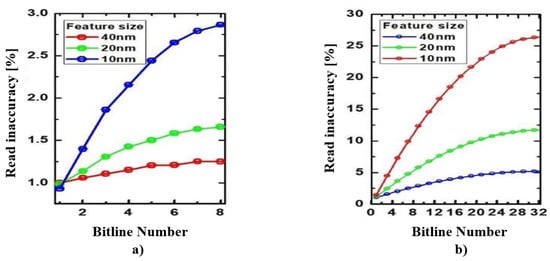
Figure 6.
An example of accuracy deviation on RRAM devices (40 nm, 20 nm, 10 nm), effected by IR drop and sneak path, in which Bitline number represents the number of channels on each layer, and read inaccuracy is accuracy deviation: (a) accruacy deviation with a number of bitline from 1 to 8; (b) accuracy deviation with a number of bitline from 1 to 32.
The Deepbit method is performed in three phases. In the first phase, for any given model, the width of the network (the number of output channels of each convolution layer) is reduced uniformly for each layer. In other words, for a given model, the width of the network remains constant across all layers. The first phase is started by defining a model with a depth equal to the minimum number in set L, while the width of the network is defined by the mentioned second input (50 for our experiments). The binary search algorithm is used to explore the BNN model with a minimal uniform width that matches the minimum accuracy threshold defined in the third input to our method. The algorithm for phase 1 is explained in Algorithm 1.
More specifically, the result of Algorithm 1 is , which is the minimum uniform width for the model with a certain number of layers. Meanwhile, inputs of the algorithm are from the second input of the Deepbit, (the number of convolution layers of the searching model), and , which is the accuracy threshold (the third input of the Deepbit). To start the searching process in this algorithm, firstly, a range of model width is initialized (). Next, a binary searching process is performed on this range until . During the binary searching process, the model with the width being the midpoint of the range is trained. If the accuracy is better than the accuracy threshold, the upper half of the searching range is selected for the subsequent searching round. By contrast, the lower half of the range would be selected for the subsequent searching round. The final output , corresponding to the certain number of layers, is stored to use for the second phase.
In the second phase, our method tries to find the optimal width for each layer. This method is performed on the output of phase 1. In this phase, the uniform width of our network is reduced to the minimum width of the network found in phase 1. A binary search is used again to find the optimal width for the first layer, while the width for the other layers is set constant to the optimal uniform width. Once the optimal width for the first layer is found, searching the optimal widths of the rest layers is performed with the same process. During the search for a typical layer, the widths of the rest layers need to be kept with the initial value, even for those that have performed the optimal width search. All optimal width values for all convolution layers are stored and resumed for the next phase of the searching method. The algorithm for phase 2 is described in Algorithm 2. Similar to Algorithm 1, the searching process is performed in an initial range, in which is the from phase 1, and is zero. However, as mentioned before, the searching is executed for each layer while keeping other ones with the .
| Algorithm 1: Optimal uniform channel search for a given BNN model |
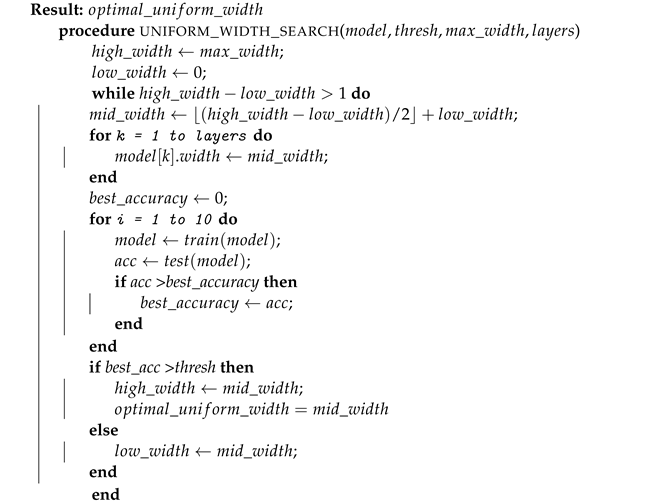 |
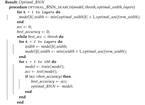
In the third phase, which is also the final phase of the searching method, the of each layer from the second phase is used to define the optimal BNN model. Since all the layers were set to a uniform width while searching for an optimal width for a specific layer, the desirable accuracy degradation can be expected when combining all of the s of each layer. To compensate for the accuracy loss, the width of each layer is increased by two more channels for each layer. If the width of each layer is greater than the model’s in the first phase, the is applied for this layer instead of using the optimal value plus 2. The next step is the training process on the new BNN model with reconfigured width values. If the accuracy matches the threshold accuracy, the model is selected as the optimal BNN model with the given initial depth. If the accuracy is below the threshold, the width of each layer continues to increase one, and the model is retrained to check the accuracy. This process is repeated until the optimal model with accuracy matching the threshold is achieved, or the width of any layer is equal to the in phase 1. This process is repeated for all the depth values in set L. Consequently, a series of BNN models with optimal width configurations and variable depths is produced. In our experiments, we keep the depth of the network from 3 to 8. The algorithm for phase 3 is explained in Algorithm 3. More specifically, at the beginning, the width of each layer is updated with . In the while loop, the width of each layer is increased one to ensure increasing two for initialization. After training 100 times, the best model and corresponding accuracy are stored. If the best accuracy is less than the accuracy threshes, the training process is repeated until we obtain the model with better accuracy than the accuracy threshold.
| Algorithm 2: Optimal width search for a given BNN model |
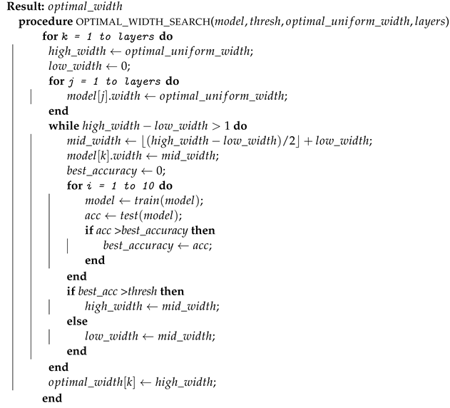 |
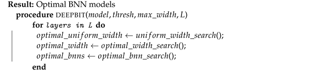
In summary, the entire Deepbit algorithm is summarized in Algorithm 4. More specifically, based on the initial inputs, including the number of layers, accuracy threshold, and initial max-width, the procedure is used to explore (phase 1). Then, the is used to find the for each layer by using the procedure (phase 2). Finally, the of all layers are used to construct a unique model, and this model is continuously optimized with the procedure until we have the minimum width for each layer, and this final model satisfies the accuracy threshold (phase 3).
| Algorithm 3: Optimal BNN search based on optimal width configuration |
 |
The output of the Deepbit algorithm is a list of optimal BNN models. Each model corresponds to a certain number of layers in the L input list. To find the most hardware-friendly model based on this series of optimal BNN models, the target hardware costs for each model are estimated according to the hardware cost estimation method introduced in the previous subsection. Typically, every model uses a uniform width in the hardware cost charts to represent the number of channels per layer. This means the number of channels per layer is the same as the model’s uniform width. Hence, to evaluate the hardware cost for an optimal model, the average number of channels per layer can play the same role as the model’s optimal width and can be used to search the optimal model based on the hardware estimation charts. Because the estimation charts do not show all hardware costs for all optimal width values, the linear regression method can be further used to estimate the target hardware cost for each model. When more than two models have the same average number of channels per layer during the searching process, the corresponding hardware designs are implemented to evaluate them correctly. After the entire process, the optimal BNN model will be selected, which has the minimum hardware cost.
| Algorithm 4: Deepbit Architecture search algorithm |
 |
5. Experimental Results and Discussion
In this section, some experiments are conducted to demonstrate the effectiveness of the proposed method. GPUs, RRAM, and FPGA are target platforms to find optimal BNN architectures. Depending on the type of target platforms, the corresponding Hardware Cost Estimation is prepared for the sensitive resources.
For FPGA devices, the BNN architecture is implemented on the Ultra96 evaluation Board, which includes an xczu3eg-sbva484-1-e Ultrascale+ MPSoC. In particular, the Process Subsystem (PS) comprises a quad-core Arm Cortex-A53 application processing unit and a dual-core Arm Cortex-R5 real-time processing unit. In the programmable logic (PL), there are 141,120 flip-flops, 70,560 LUTs, 360 DSP slices, and 7.6 Mbits block ram. The register-transfer level (RTL) design is simulated on Synopsys VCS, then synthesis and implementation are executed on Vivado 2018.3. All experiment results describing the number of LUTS, flip-flops, and estimated power consumption is collected from Vivado’s report. For RRAM devices, as introduced in previous sections, an error simulation is prepared for the training process and inference period. Meanwhile, for the GPU experiments and training task, we use RTX 2080ti to find the model with the best accuracy on this device.
5.1. Optimal BNN Search
Based on the basic design strategies defined in Section 3 and the Deepbit method, in this subsection, the searching process performed on our experiments with a specific configuration is described. In addition, the corresponding results are also shown to prove the efficiency of the proposed method. In particular, for FPGA, the target for the optimal BNN architecture is 98.4% accuracy with minimal hardware resources. Meanwhile, the target for GPU and RRAM is simply developing a BNN architecture with maximum accuracy. As mentioned in the previous section, the Deepbit method takes three inputs:
- L = {3, 4, 5, 6, 7, 8}
- maximum number of channels = 50
- minimum accuracy threshold = 98.4%
In terms of the training process, a combination of the Adam and SGD optimizer is applied. More specifically, the SGD optimizer is used for the 100 epochs. The learning rate and momentum are set at 0.03 and 0.5, respectively. Each training is conducted 10 times for phase 1 and phase 2 of the architectural search method. In the final phase, at the time searching for the final model, the training has repeated a total of 10 times. Six required optimal BNN models correspond to a depth from 3 to 8. The width configuration for each model is defined in Table 5. On the other hand, as mentioned in Section 3, a layer module for BNN models is depicted in Figure 2. Each module comprises a convolution operation followed by a batch norm and a Tanh activation function. Moreover, the last two convolution layers comprise the Max pooling layer, and the last layer of all BNN models is always the fully connected layer. Finally, the optimal width for each layer of our BNN models is found by the Deepbit architecture search method.
Table 5.
The width configuration of optimal BNNs found by Deepbit method.
5.2. Estimating the Hardware Costs for Optimal Models
To estimate the hardware costs, the most sensitive hardware resources depending on each hardware platform are selected and estimated based on the method described in Section 4. In particular, for FPGA, Look Up Tables, flip-flops, and power consumption are selected to estimate the hardware cost. The range for network depth and width is the follows.
All the possible models with depth and width defined by the set L and C are initialized with random weight values. Next, these models are physically tested on corresponding target hardware platforms. Based on the implemented results, hardware estimation charts are prepared for the searching method. In Table 6, Table 7 and Table 8, the cost estimation charts based on Look Up Tables, flip-flops, and power consumption are provided for FPGA platforms. Specifically, the actual hardware costs for various models with a width interval of five channels are prepared prior. As mentioned in the previous section, in a cost estimation chart, because each model has a uniform width for each layer, the average width per layer is considered the uniform width of optimal BNN models. The actual hardware cost for the optimal model can be found with a uniform width and the number of layers existing in the hardware cost estimation chart. In this case, if the optimal width is not in the estimation chart, linear interpolation can be applied to estimate the hardware cost of the optimal model. For example, with the three layers optimal model, as shown in Table 5. The average width per layer for this model is 27. The cost estimation chart shows hardware cost C1 for BNN models with 25 channels per layer and C2 for BNN models with 30 channels per layer. Finally, the hardware cost for model (C_est) is estimated with linear interpolation as the following equation:
Table 6.
LUT estimation charts.
Table 7.
Flip-flop estimation charts.
Table 8.
Power consumption estimation charts.
In Table 9, the hardware costs of the optimal BNN models found by the estimated method are provided. Accordingly, the model with four layers consumes the lowest number of LUTs (18,764) and energy (1.151), while flip-flop is consumed the least by the model with three layers. By comparing the number of MAC operations among optimal models, we can conclude that the model with the minimum number of MAC operations may or may not be the optimal one for hardware implementation on FPGA. Therefore, estimating the actual hardware costs for software models is significant in exploring the best model for implementation on any specific target platform.
Table 9.
Hardware cost estimates for the optimized BNN models.
Regarding GPU and RRAM devices, the accuracy is the only target for architecture search in the scope of experiments. Thus, optimal BNN models, which have maximum accuracy, are the output of the architecture search for GPUs and RRAM. In particular, the accuracy charts for GPU are described in Table 3. Different from other devices, the computational cost on GPU depends on the number of MAC operations. Hence, the optimal BNN model would have the fewest number of MAC operations and the highest accuracy. According to Table 3, the accuracy tends to saturate when the number of channels exceeds 40, and the number of layers is more than 5. Accordingly, increasing the number of channels or layers (leading to increased MAC operations) in this experiment does not constantly improve accuracy and can be a burden for the computation. Based on observations, the optimal BNN model for GPU is the model with 6 convolution layers and 50 output channels that give the best accuracy (98.88%) and an optimal number of MAC operations.
For RRAM devices, a simulator is prepared to emulate the RRAM’s working mechanism, in which errors are caused by I/R drop and white noise is injected into the simulator. Theoretically, more channels give a considerable error in a convolution layer implemented on RRAM devices. With this characteristic, the simulation is performed, and the accuracy estimation is provided in Table 10 for RRAM devices. Accordingly, even though the effect of RRAM error is minimal, 10 channels are not enough to provide high accuracy. Meanwhile, the error shows that the models with 50 channels are significantly affected. Thus, the accuracy is not improved with too many channels per layer. Based on this observation, the model with 7 layers and 30 channels has the best performance, i.e., 98.45%, and it is considered the optimal candidate for RRAM-based devices.
Table 10.
RRAM accuracy estimation charts.
5.3. Analysis and Discussion
The optimal model selected can be different depending on the target cost estimation. For FPGA, as shown in Table 9, the model with three layers has the fewest flip-flops, while the model with four layers has the fewest LUTs and consumes the lowest power consumption. If the power consumption is considered the most critical resource, the model with four layers will be the optimal candidate.
Table 11 shows the real hardware cost for our best model. Compares the hardware costs of the selected model with md1, which has the fewest MAC operations, we can see that the proposed method can reduce the power consumption of the target hardware compared to using MAC operations. In addition, according to Table 9, the estimation method gives valuable data related to the hardware cost compared to actual hardware overhead. Therefore, the network designs can be considerably optimized on the critical cost when applying the proposed method for complex networks and datasets. For example, in our experiments, the model md4 with six convolution layers has almost 1.5 times more MAC operations than the model with three layers but has similar hardware statistics as the model with three layers. This result is proof that MAC operations can be misleading and not a reasonable estimate for actual hardware performance.
Table 11.
Comparison of actual hardware performance and MAC operations of various models.
Finally, the optimal BNN models found by our method for the different target hardware in this paper are provided in Table 12. Based on this table, there is a conclusion that the optimal network architecture is different for each hardware, and it is not possible to find an optimal network for any hardware using generalized metrics, such as FLOPs or MAC operations. Each hardware has different critical resources, and we need hardware-specific metrics to find an optimal model for the target hardware.
Table 12.
Optimal BNN models for different hardwares.
5.4. Future Work
Based on the final evaluation result, the presented solution has shown effectiveness in exploring the optimal BNN models for different hardware platforms and different critical hardware requirements. In particular, each hardware platform is provided a different optimal BNN model, which does not have the minimum number of MACs but would be the best one for the target requirements. However, with the MNIST, a small dataset, the proposed algorithm has not shown comprehensive benefits, and many potential issues that occur with more extensive datasets may not be solved. Because of the complexity in simulating the error affected by the IR drop and sneak path, the estimation charts for RRAM devices on more extensive datasets are not available. Therefore, in future work, Cifar-10 and ImageNet are going to be the next target datasets for the searching process. In particular, to reduce the searching time, which may be the biggest drawback of the proposed solution for an extensive dataset, the number of training times can be reduced for each model in Algorithm 3 (100 for MNIST dataset). In addition, in Algorithm 3, instead of adding two more channels for initialization and one channel to compensate for the accuracy in the while-loop, 64 channels can be used for initialization and 32 channels for the while-loop. In terms of exploring the range of layers for the searching process, as introduced in Section 4.2, there can be more steps for the increasing number of layers and channels for bigger datasets.
6. Conclusions
Optimizing DNN models for hardware implementation has been challenging, especially for applications with resource-constrained embedded environments. Although BNN, one of the prior approaches, can considerably simplify Neural Network models, the accuracy degradation is still a drawback when binarizing weights and activations. In addition to deploying optimal accelerators and optimizing based on accuracy and generalized metrics, such as FLOPs, MAC operations are also a popular method applied for most neural network models. However, each hardware platform has different characteristics. Thus, only evaluating on software level is not enough to select the optimal model for hardware implementation. This paper has successfully demonstrated the possibility of an architecture searching method (the Deepbit), including training strategies and hardware-cost estimation techniques, to explore the final optimal BNN model for specific hardware platforms. Typically, with the Deepbit algorithm, the scope of the searching process is narrowed. Meanwhile, based on critical resources, the hardware-cost estimation can help select better optimal BNN models for specific hardware platforms, with input being a list of BNN models, compared to independent optimization on the software level. However, as all experiments have only been conducted on a small dataset (MNIST) and simple neural networks (BNNs), various challenges need to be tackled when applying the proposed method to practical applications. Thus, Deepbit for DNNs will be deployed in future work to evaluate the feasibility of the presented solution.
Author Contributions
Conceptualization, L.K.; methodology, L.K., F.A. and Q.H.V.; validation, Q.H.V., F.A., L.K. and S.L.; formal analysis, Q.H.V. and F.A.; investigation, Q.H.V. and F.A.; resources, Q.H.V., F.A., B.A., S.L. and L.K.; writing—original draft preparation, Q.H.V., F.A. and L.K.; writing—review and editing, Q.H.V., F.A., B.A., S.L. and L.K.; visualization, Q.H.V. and F.A.; supervision, L.K. and S.L.; funding acquisition, L.K. and S.L. All authors have read and agreed to the published version of the manuscript.
Funding
This research was supported by the National R&D Program through the National Research Foundation of Korea (NRF) funded by the Ministry of Science and ICT (2020M3F3A2A01085755) and the technology innovation program (No. 10085646) funded by the Ministry of Trade, Industry, and Energy (MOTIE, Korea).
Institutional Review Board Statement
Not applicable.
Informed Consent Statement
Not applicable.
Data Availability Statement
Not applicable.
Conflicts of Interest
The authors declare no conflict of interest.
References
- Voulodimos, A.; Doulamis, N.; Doulamis, A.; Protopapadakis, E.; Andina, D. Deep Learning for Computer Vision: A Brief Review. Intell. Neurosci. 2018, 2018, 7068349. [Google Scholar] [CrossRef]
- Nassif, A.B.; Shahin, I.; Attili, I.; Azzeh, M.; Shaalan, K. Speech recognition using deep neural networks: A systematic review. IEEE Access 2019, 7, 19143–19165. [Google Scholar] [CrossRef]
- LeCun, Y.; Denker, J.S.; Solla, S.A. Optimal brain damage. In Advances in Neural Information Processing Systems; Touretzky, D., Ed.; Morgan-Kaufmann: San Mateo, CA, USA, 1990; pp. 598–605. [Google Scholar]
- Han, S.; Pool, J.; Tran, J.; Dally, W.J. Learning both weights and connections for efficient neural networks. arXiv 2015, arXiv:1506.02626. [Google Scholar]
- Han, S.; Mao, H.; Dally, W.J. Deep compression: Compressing deep neural networks with pruning, trained quantization and huffman coding. arXiv 2015, arXiv:1510.00149. [Google Scholar]
- Lin, D.; Talathi, S.; Annapureddy, S. Fixed point quantization of deep convolutional networks. In Proceedings of the International Conference on Machine Learning, New York, NY, USA, 20–22 June 2016; pp. 2849–2858. [Google Scholar]
- Wu, J.; Leng, C.; Wang, Y.; Hu, Q.; Cheng, J. Quantized convolutional neural networks for mobile devices. In Proceedings of the IEEE Conference on Computer Vision and Pattern Recognition, Las Vegas, NV, USA, 27–30 June 2016; pp. 4820–4828. [Google Scholar]
- Courbariaux, M.; Bengio, Y.; David, J.P. Binaryconnect: Training deep neural networks with binary weights during propagations. In Advances in Neural Information Processing Systems; Curran Associates, Inc.: Montreal, QC, Canada, 2015; pp. 3123–3131. [Google Scholar]
- Rastegari, M.; Ordonez, V.; Redmon, J.; Farhadi, A. Xnor-net: Imagenet classification using binary convolutional neural networks. In European Conference on Computer Vision; Springer: Berlin/Heidelberg, Germany, 2016; pp. 525–542. [Google Scholar]
- Courbariaux, M.; Hubara, I.; Soudry, D.; El-Yaniv, R.; Bengio, Y. Binarized neural networks: Training deep neural networks with weights and activations constrained to+ 1 or -1. arXiv 2016, arXiv:1602.02830. [Google Scholar]
- Tang, W.; Hua, G.; Wang, L. How to train a compact binary neural network with high accuracy? In Proceedings of the Thirty-First AAAI Conference on Artificial Intelligence, San Francisco, CA, USA, 4–9 February 2017. [Google Scholar]
- Lin, X.; Zhao, C.; Pan, W. Towards accurate binary convolutional neural network. arXiv 2017, arXiv:1711.11294. [Google Scholar]
- Liu, Z.; Shen, Z.; Savvides, M.; Cheng, K.T. Reactnet: Towards precise binary neural network with generalized activation functions. In European Conference on Computer Vision; Springer: Berlin/Heidelberg, Germany, 2020; pp. 143–159. [Google Scholar]
- Lin, M.; Ji, R.; Xu, Z.; Zhang, B.; Wang, Y.; Wu, Y.; Huang, F.; Lin, C.W. Rotated binary neural network. arXiv 2020, arXiv:2009.13055. [Google Scholar]
- Blott, M.; Preußer, T.B.; Fraser, N.J.; Gambardella, G.; O’brien, K.; Umuroglu, Y.; Leeser, M.; Vissers, K. FINN-R: An end-to-end deep-learning framework for fast exploration of quantized neural networks. ACM Trans. Reconfigurable Technol. Syst. (TRETS) 2018, 11, 1–23. [Google Scholar] [CrossRef]
- Umuroglu, Y.; Fraser, N.J.; Gambardella, G.; Blott, M.; Leong, P.; Jahre, M.; Vissers, K. Finn: A framework for fast, scalable binarized neural network inference. In Proceedings of the 2017 ACM/SIGDA International Symposium on Field-Programmable Gate Arrays, Monterey, CA, USA, 22–24 February 2017; pp. 65–74. [Google Scholar]
- Liang, S.; Yin, S.; Liu, L.; Luk, W.; Wei, S. FP-BNN: Binarized neural network on FPGA. Neurocomputing 2018, 275, 1072–1086. [Google Scholar] [CrossRef]
- Fu, C.; Zhu, S.; Su, H.; Lee, C.E.; Zhao, J. Towards fast and energy-efficient binarized neural network inference on fpga. arXiv 2018, arXiv:1810.02068. [Google Scholar]
- Sun, X.; Yin, S.; Peng, X.; Liu, R.; Seo, J.S.; Yu, S. XNOR-RRAM: A scalable and parallel resistive synaptic architecture for binary neural networks. In Proceedings of the 2018 Design, Automation & Test in Europe Conference & Exhibition (DATE), Dresden, Germany, 19–23 March 2018; pp. 1423–1428. [Google Scholar]
- Yin, S.; Jiang, Z.; Seo, J.S.; Seok, M. XNOR-SRAM: In-memory computing SRAM macro for binary/ternary deep neural networks. IEEE J.-Solid-State Circuits 2020, 55, 1733–1743. [Google Scholar] [CrossRef]
- Agrawal, A.; Jaiswal, A.; Roy, D.; Han, B.; Srinivasan, G.; Ankit, A.; Roy, K. Xcel-RAM: Accelerating binary neural networks in high-throughput SRAM compute arrays. IEEE Trans. Circuits Syst. I Regul. Pap. 2019, 66, 3064–3076. [Google Scholar] [CrossRef] [Green Version]
- Khwa, W.S.; Chen, J.J.; Li, J.F.; Si, X.; Yang, E.Y.; Sun, X.; Liu, R.; Chen, P.Y.; Li, Q.; Yu, S.; et al. A 65 nm 4 Kb algorithm-dependent computing-in-memory SRAM unit-macro with 2.3 ns and 55.8 TOPS/W fully parallel product-sum operation for binary DNN edge processors. In Proceedings of the 2018 IEEE International Solid-State Circuits Conference-(ISSCC), San Francisco, CA, USA, 11–15 February 2018; pp. 496–498. [Google Scholar]
- Kim, H.; Sim, J.; Choi, Y.; Kim, L.S. A kernel decomposition architecture for binary-weight convolutional neural networks. In Proceedings of the 54th Annual Design Automation Conference 2017, Austin, TX, USA, 18–22 June 2017; pp. 1–6. [Google Scholar]
- Alwani, M.; Chen, H.; Ferdman, M.; Milder, P. Fused-layer CNN accelerators. In Proceedings of the 2016 49th Annual IEEE/ACM International Symposium on Microarchitecture (MICRO), Taipei, Taiwan, 15–19 October 2016; pp. 1–12. [Google Scholar]
- Chen, Y.H.; Krishna, T.; Emer, J.S.; Sze, V. Eyeriss: An energy-efficient reconfigurable accelerator for deep convolutional neural networks. IEEE J.-Solid-State Circuits 2016, 52, 127–138. [Google Scholar] [CrossRef] [Green Version]
- Lu, L.; Liang, Y. SpWA: An efficient sparse winograd convolutional neural networks accelerator on FPGAs. In Proceedings of the 55th Annual Design Automation Conference, San Francisco, CA, USA, 24–29 June 2018; pp. 1–6. [Google Scholar]
- Lu, L.; Liang, Y.; Xiao, Q.; Yan, S. Evaluating fast algorithms for convolutional neural networks on FPGAs. In Proceedings of the 2017 IEEE 25th Annual International Symposium on Field-Programmable Custom Computing Machines (FCCM), Napa, CA, USA, 30 April–2 May 2017; pp. 101–108. [Google Scholar]
- Qiu, J.; Wang, J.; Yao, S.; Guo, K.; Li, B.; Zhou, E.; Yu, J.; Tang, T.; Xu, N.; Song, S.; et al. Going deeper with embedded fpga platform for convolutional neural network. In Proceedings of the 2016 ACM/SIGDA International Symposium on Field-Programmable Gate Arrays, Monterey, CA, USA, 21–23 February 2016; pp. 26–35. [Google Scholar]
- Wei, X.; Liang, Y.; Li, X.; Yu, C.H.; Zhang, P.; Cong, J. TGPA: Tile-grained pipeline architecture for low latency CNN inference. In Proceedings of the International Conference on Computer-Aided Design, San Diego, CA, USA, 5–8 November 2018; pp. 1–8. [Google Scholar]
- Wei, X.; Yu, C.H.; Zhang, P.; Chen, Y.; Wang, Y.; Hu, H.; Liang, Y.; Cong, J. Automated systolic array architecture synthesis for high throughput CNN inference on FPGAs. In Proceedings of the 54th Annual Design Automation Conference 2017, Austin, TX, USA, 18–22 June 2017; pp. 1–6. [Google Scholar]
- Xiao, Q.; Liang, Y.; Lu, L.; Yan, S.; Tai, Y.W. Exploring heterogeneous algorithms for accelerating deep convolutional neural networks on FPGAs. In Proceedings of the 54th Annual Design Automation Conference 2017, Austin, TX, USA, 18–22 June 2017; pp. 1–6. [Google Scholar]
- Zhang, C.; Li, P.; Sun, G.; Guan, Y.; Xiao, B.; Cong, J. Optimizing fpga-based accelerator design for deep convolutional neural networks. In Proceedings of the 2015 ACM/SIGDA International Symposium on Field-Programmable Gate Arrays, Monterey, CA, USA, 22–24 February 2015; pp. 161–170. [Google Scholar]
- Zoph, B.; Le, Q.V. Neural architecture search with reinforcement learning. arXiv 2016, arXiv:1611.01578. [Google Scholar]
- Zoph, B.; Vasudevan, V.; Shlens, J.; Le, Q.V. Learning transferable architectures for scalable image recognition. In Proceedings of the IEEE Conference on Computer Vision and Pattern Recognition, Salt Lake City, UT, USA, 18–22 June 2018; pp. 8697–8710. [Google Scholar]
- Stamoulis, D.; Cai, E.; Juan, D.C.; Marculescu, D. Hyperpower: Power- and memory-constrained hyper-parameter optimization for neural networks. In Proceedings of the 2018 Design, Automation & Test in Europe Conference & Exhibition (DATE), Dresden, Germany, 19–23 March 2018; pp. 19–24. [Google Scholar]
- Tan, M.; Chen, B.; Pang, R.; Vasudevan, V.; Sandler, M.; Howard, A.; Le, Q.V. MnasNet: Platform-Aware Neural Architecture Search for Mobile. In Proceedings of the CVF Conference on Computer Vision and Pattern Recognition (CVPR), Salt Lake City, UT, USA, 18–23 June 2018; pp. 2815–2823. [Google Scholar]
- Wu, B.; Dai, X.; Zhang, P.; Wang, Y.; Sun, F.; Wu, Y.; Tian, Y.; Vajda, P.; Jia, Y.; Keutzer, K. Fbnet: Hardware-aware efficient convnet design via differentiable neural architecture search. In Proceedings of the IEEE/CVF Conference on Computer Vision and Pattern Recognition, Long Beach, CA, USA, 15–20 June 2019; pp. 10734–10742. [Google Scholar]
- Guo, Z.; Zhang, X.; Mu, H.; Heng, W.; Liu, Z.; Wei, Y.; Sun, J. Single path one-shot neural architecture search with uniform sampling. In European Conference on Computer Vision; Springer: Berlin/Heidelberg, Germany, 2020; pp. 544–560. [Google Scholar]
- Chu, X.; Zhang, B.; Xu, R. Fairnas: Rethinking evaluation fairness of weight sharing neural architecture search. In Proceedings of the IEEE/CVF International Conference on Computer Vision, Montreal, QC, Canada, 11–17 October 2021; pp. 12239–12248. [Google Scholar]
- Cai, H.; Zhu, L.; Han, S. Proxylessnas: Direct neural architecture search on target task and hardware. arXiv 2018, arXiv:1812.00332. [Google Scholar]
- Stamoulis, D.; Ding, R.; Wang, D.; Lymberopoulos, D.; Priyantha, B.; Liu, J.; Marculescu, D. Single-path nas: Designing hardware-efficient convnets in less than 4 hours. arXiv 2019, arXiv:1904.02877. [Google Scholar]
- Wang, K.; Liu, Z.; Lin, Y.; Lin, J.; Han, S. Haq: Hardware-aware automated quantization with mixed precision. In Proceedings of the IEEE/CVF Conference on Computer Vision and Pattern Recognition, Long Beach, CA, USA, 15–20 June 2019; pp. 8612–8620. [Google Scholar]
- Tan, M.; Chen, B.; Pang, R.; Vasudevan, V.; Sandler, M.; Howard, A.; Le, Q.V. Mnasnet: Platform-aware neural architecture search for mobile. In Proceedings of the IEEE/CVF Conference on Computer Vision and Pattern Recognition, Long Beach, CA, USA, 15–20 June 2019; pp. 2820–2828. [Google Scholar]
- Google. Edge TPU. Available online: https://cloud.google.com (accessed on 20 November 2021).
- Hruska, J. New Movidius Myriad X VPU Packs a Custom Neural Compute Engine. August 2017. Available online: https://www.extremetech.com/computing/254772-new-movidiusmyriad-x-vpu-packs-custom-neural-compute-engine (accessed on 20 November 2021).
- Hruska, J. Nvidia’s Jetson Xavier Stuffs Volta Performance into Tiny Form Factor. June 2018. Available online: https://www.extremetech.com/computing/270681-nvidias-jetsonxavier-stuffs-volta-performance-into-tiny-form-factor (accessed on 20 November 2021).
- Benmeziane, H.; Maghraoui, K.E.; Ouarnoughi, H.; Niar, S.; Wistuba, M.; Wang, N. A Comprehensive Survey on Hardware-Aware Neural Architecture Search. arXiv 2021, arXiv:2101.09336. [Google Scholar]
- Smithson, S.C.; Yang, G.; Gross, W.J.; Meyer, B.H. Neural networks designing neural networks: Multi-objective hyper-parameter optimization. In Proceedings of the 35th International Conference on Computer-Aided Design, Austin, TX, USA, 7–10 November 2016; pp. 1–8. [Google Scholar]
- Gordon, A.; Eban, E.; Nachum, O.; Chen, B.; Wu, H.; Yang, T.J.; Choi, E. Morphnet: Fast & simple resource-constrained structure learning of deep networks. In Proceedings of the IEEE Conference on Computer Vision and Pattern Recognition, Salt Lake City, UT, USA, 18–22 June 2018; pp. 1586–1595. [Google Scholar]
- Dong, J.D.; Cheng, A.C.; Juan, D.C.; Wei, W.; Sun, M. Ppp-Net: Platform-Aware Progressive Search for Pareto-Optimal Neural Architectures. In Proceedings of the International Conference on Learning Representations, Vancouver, BC, Canada, 30 April–3 May 2018. [Google Scholar]
- Elsken, T.; Metzen, J.H.; Hutter, F. Efficient multi-objective neural architecture search via lamarckian evolution. arXiv 2018, arXiv:1804.09081. [Google Scholar]
- Zhou, Y.; Ebrahimi, S.; Arık, S.Ö.; Yu, H.; Liu, H.; Diamos, G. Resource-efficient neural architect. arXiv 2018, arXiv:1806.07912. [Google Scholar]
- Hsu, C.H.; Chang, S.H.; Liang, J.H.; Chou, H.P.; Liu, C.H.; Chang, S.C.; Pan, J.Y.; Chen, Y.T.; Wei, W.; Juan, D.C. Monas: Multi-objective neural architecture search using reinforcement learning. arXiv 2018, arXiv:1806.10332. [Google Scholar]
- Li, J.; Diao, W.; Sun, X.; Feng, Y.; Zhang, W.; Chang, Z.; Fu, K. Automated and lightweight network design via random search for remote sensing image scene classification. Int. Arch. Photogramm. Remote Sens. Spat. Inf. Sci. 2020, 43, 1217–1224. [Google Scholar] [CrossRef]
- Zhang, L.L.; Yang, Y.; Jiang, Y.; Zhu, W.; Liu, Y. Fast hardware-aware neural architecture search. In Proceedings of the IEEE/CVF Conference on Computer Vision and Pattern Recognition Workshops, Seattle, WA, USA, 14–19 June 2020; pp. 692–693. [Google Scholar]
- Gupta, S.; Akin, B. Accelerator-aware neural network design using automl. arXiv 2020, arXiv:2003.02838. [Google Scholar]
- Cai, H.; Gan, C.; Wang, T.; Zhang, Z.; Han, S. Once-for-all: Train one network and specialize it for efficient deployment. arXiv 2019, arXiv:1908.09791. [Google Scholar]
- Laube, K.A.; Zell, A. Shufflenasnets: Efficient cnn models through modified efficient neural architecture search. In Proceedings of the 2019 International Joint Conference on Neural Networks (IJCNN), Budapest, Hungary, 14–19 July 2019; pp. 1–6. [Google Scholar]
- Woo, J.; Peng, X.; Yu, S. Design considerations of selector device in cross-point RRAM array for neuromorphic computing. In Proceedings of the 2018 IEEE International Symposium on Circuits and Systems (ISCAS), Florence, Italy, 27–30 May 2018; pp. 1–4. [Google Scholar]
- Ni, L.; Liu, Z.; Song, W.; Yang, J.J.; Yu, H.; Wang, K.; Wang, Y. An energy-efficient and high-throughput bitwise CNN on sneak-path-free digital ReRAM crossbar. In Proceedings of the 2017 IEEE/ACM International Symposium on Low Power Electronics and Design (ISLPED), Monterey, CA, USA, 10–12 August 2017; pp. 1–6. [Google Scholar]
Publisher’s Note: MDPI stays neutral with regard to jurisdictional claims in published maps and institutional affiliations. |
© 2022 by the authors. Licensee MDPI, Basel, Switzerland. This article is an open access article distributed under the terms and conditions of the Creative Commons Attribution (CC BY) license (https://creativecommons.org/licenses/by/4.0/).