Dirichlet Matrix Factorization: A Reliable Classification-Based Recommender System

Abstract

Traditionally, recommender systems have been approached as regression models aiming to predict the score that a user would give to a particular item. In this work, we propose a recommender system that tackles the problem as a classification task instead of as a regression. The new model, Dirichlet Matrix Factorization (DirMF), provides not only a prediction but also its reliability, hence achieving a better balance between the quality and quantity of the predictions (i.e., reducing the prediction error by limiting the model’s coverage). The experimental results conducted show that the proposed model outperforms other models due to its ability to discard unreliable predictions. Compared to our previous model, which uses the same classification approach, DirMF shows a similar efficiency, outperforming the former on some of the datasets included in the experimental setup.

1. Introduction

In the latest years, society is becoming more and more saturated with the overwhelming amount of information available to costumers. For this reason, the use of algorithms for information retrieval and sorting is becoming a cornerstone in the technological solutions offered. An important instance of these methods is Recommender Systems (RSs), which aid users to match with items in the most efficient way possible, taking into account both the user’s own preferences and those of others with similar tastes. An evidence of the deep penetration of these algorithms in the industry is the high number of companies that use RSs as part of their business model, such as Amazon, eBay, Netflix, Twitter and many others. However, although improving recommendation accuracy has been the main target for academic researchers [1], other objectives that are beyond improving accuracy have also attracted the interest of the community in recent years [2]. Metrics such as coverage, diversity and novelty are goals of cutting-edge research since users typically prefer to be recommended items with a certain degree of novelty. Recent RSs research suggests that accurate recommendations are possible [3]: when RSs recommend a restaurant by awarding it five stars, a human is likely to be skeptical of the rating. Some RSs provide some extra data that help us to deduce the rating’s trustworthiness such as the number of individuals who have voted for the restaurant. Almost everyone prefers a restaurant with an average rating of 4 stars and 5000 reviews to one with just 5 reviews and an average rating of 5 stars. In this framework, a recommendation does not only comprise the recommended item, but also an associated reliability value provided through RSs techniques and models for trustworthiness.

The core of every RS is its filtering mechanism. Broadly speaking, the system makes recommendations based on context [4], content [5], social environment [6], demographic data [7] and collaborative information, the latter being the most widely used approach [8]. Hybrid methods [9], which combine Collaborative Filtering (CF) and other filtering sources, are commonly used in commercial RS designs.

Among CF methods, Probabilistic Matrix Factorization (PMF) [10] is arguably the most relevant contribution to the area in the latest times. It models the process of assigning a rating as regression process that follows a normal distribution with mean given by the inner product of two ‘hidden vectors’ associated to each user and item. Since it inception, other CF models have been proposed to extend the ideas PMF to work with more general frameworks. One of the most promising lines is to combine the hidden vectors in a non-linear way, in sharp contrast with the usual operation of PMF. For instance, in [11], two new models are proposed inspired by deep learning techniques, namely, Generalized Matrix Factorization (GMF) and Neural Collaborative Filtering (NCF). In the former, instead of the standard inner product in the euclidean space, a more general inner product is allowed, which is learned during the training process. To definitely break with linearity, this work also proposes NCF, in which the inner product is fully substituted by a neural network able to combine the hidden vectors in a highly non-linear way.

Despite these advances, recent works show that, in the RSs field, providing precise reliability values that are connected with forecasts is a major aim, as it provides many advantages: new ways of providing recommendations to the user that take into account the reliability of the prediction, achieving better accuracy by filtering low reliability recommendations, and identifying a cold start problem when every recommendation for an user has low reliability. It is worth noticing that reliability and accuracy are different metrics of the performance of an RS: accuracy is the objective ability of the RS of issuing correct predictions (in the sense that they agree with the known values of the test split dataset), while reliability is a subjective perception of the model on the probability that its prediction is correct. In some sense, reliability measures the impression of the algorithm on the ‘difficulty’ of issuing the prediction. In this way, a good RS method labels controvert predictions with low reliability while clear trends are associated to high reliability. This reliability measure can be used to filter-out these controvert predictions, in such a way that only forecasts with high reliability are issued. If the RS models reliability correctly, this filtration will lead to an improvement of the accuracy of the predictions.

For this reason, several CF-based methods and models have been developed to provide reliability values based on both the Matrix Factorization (MF) and K Nearest Neighbors (KNN) approaches, in contrast with the aforementioned proposals which do not support this metric. For instance, Margaris et al. [12] presents the notion of reliability in the domain of review-to-rating conversion, that is, the reliability of converting textual reviews to implicit ratings. In addition, Mesas and Bellogín [13] looks at a few different ways of embedding awareness in an RS to analyze whether each item should be offered. The authors claim that, similar to our suggested strategy, confidence values may be used to filter the most trustworthy recommendations, resulting in an increase in accuracy and a drop in coverage.

Regarding memory-based approaches, Fan et al. [14] improves classic Pearson and cosine similarity metrics by applying the reliability concept. Previously, authors calculated the credibility of a user’s rating using the users’ scores on common products. Ahmadian et al. [15] presented an aggregation of reliability metrics, including user-based reliability, rating profile reliability, and item-based reliability. Their model is able to make better suggestions as a result of this knowledge. Liang et al. [16], Xu et al. [17] both used an upper bound of confidence to improve recommendations, the former using event-based social networks and synthetic datasets, and the latter exploiting the user’s behavior temporal information to improve the accuracy of the recommendations.

Despite its effectiveness, the above-mentioned studies have two major flaws in terms of dependability. First, because of its lack of precision and scalability, the KNN technique is not used. Second, because social information is only available in a tiny portion of current RSs, social-based trust-aware techniques aimed at determining dependability values cannot be termed universal solutions.

In this direction, our previous model Bernoulli Matrix Factorization (BeMF) [18] addressed the problem of providing accurate recommendations in addition to their associated reliability as a classification problem. This classification approach uses a finite set of ratings that should be assigned to the items as classes to predict. In this manner, the model returns the probability that a user would assign each of the D possible ratings to an item, which was modeled as D independent Bernoulli processes. Those D probabilities can be aggregated to obtain the expected reliability result, in such a way that the model provides additional information to the recommendations.

Although our previous model achieves good results, we modeled the ratings as a D-dimensional vector of independent Bernoulli random variables, which is a rather strong assumption. To address this issue, in this work we propose a novel MF model that provides the reliability of the recommendations by using a classification-based approach. However, instead of assuming independence between the ratings, our novel proposal models them as a Dirichlet random variable to deal with the existing interdependence. Due to the key role that the Dirichlet distribution plays in the formulation of the model, as well as its crucial use of matrix factorization procedures, this new method is referred to as Dirichlet Matrix Factorization (DirMF).

The structure of this paper is as follows. Section 2 explains the interstices of the proposed DirMF model, both regarding the mathematical formulation of the underlying classification problem (Section 2.1) and the way in which prediction value and reliability can be extracted from these data (Section 2.2). The presentation is complemented with a discussion of the time and space complexity of the proposed method in Section 2.3, as well as a detailed running example shown in Section 2.4. In Section 3 we present the experiments conducted to evaluate the performance of DirMF. In particular, Section 3.1 describes the experimental setting, whereas Section 3.2 analyzes the obtained results. The paper finishes with some conclusions and future works, as outlined in Section 4.

Our Contribution

The main results and novel proposals developed in the present manuscript are the following:

• A new model, named DirMF, is introduced, and a complete description of its mathematical formulation, training procedure and prediction protocol is provided.
• The new DirMF model introduces a new probabilistic interpretation of the rating process. Instead of considering the rating as a continuous random variable or seeing each vote as an independent feature, as in the existing literature, our method is flexible enough to model the ratings as interrelated discrete random variables. For this purpose, the method proposes the novelty of relying in the Dirichlet probability distribution to model the user’s rating behavior;
• The performance of this new model is evaluated through an extensive collection of experiments. The results evidence that DirMF achieves a high performance both in terms of recommendation quality and management of reliability. The implementation of the reliability as an intrinsic part of the algorithm leads to a better performance of this method compared to the preexisting algorithms that do not treat reliability in this way;
• Additionally, DirMF shows similar results to BeMF, the other method that embeds the reliability as part of its training process. Furthermore, thanks to its more flexible nature, DirMF presents a more conservative forecasting trend than BeMF, which leads to a better prediction in scenarios in which failure is highly penalized.

2. Proposed Model

Let us assume that there are N users that may rate M different items. Rating means a user can assign a score to an item chosen from a discrete set of scores $\mathcal{S}=\left\{s_1,\dots ,s_D\right\}$. For instance, a rating consisting of giving one to five stars means $\mathcal{S}=\left\{1,2,3,4,5\right\}$. The ratings that are known are represented by the ratings matrix $R=\left(R_{u,i}\right)$, where $R_{u,i}=s$ if user $u\in [1,N]$ has assigned the score $s\in \mathcal{S}$ to item $i\in [1,M]$ and $R_{u,i}=•$ if user u has not rated item i. The matrix R is decomposed into D binary matrices $R^{s_1},\dots ,R^{s_D}$, such that $R_{u,i}^s=1$ if user u assigned the score s to item i (i.e., $R_{u,i}=s$), $R_{u,i}^s=0$ if user u assigned other score than s to the item i (i.e., $R_{u,i}\ne s$), and $R_{u,i}^s=•$ if the user u did not rate the item i (i.e., $R_{u,i}=•$).

As stated above, predicting those missing values of $R^s$ is a classification problem, as $R_{u,i}^s$ means whether user u thought that a rating of s is the best for item i. The aim of our proposal is to model the random vector $(R_{u,i}^{s_1},\dots ,R_{u,i}^{s_D})$ as a Dirichlet random variable with parameters $0\le {\rho }_{u,i}^{s_1},\dots ,{\rho }_{u,i}^{s_D}\le 1$. Therefore, $R_{u,i}^s$ quantifies both the affinity of the user u for item i and the reliability of the prediction.

Regarding how our model estimates the parameters ${\rho }_{u,i}^s$, it supposes that there exists some K-dimensional hidden user factors vector $P_u^s=(P_{u,1}^s,\dots ,P_{u,K}^s)\in {\mathbb{R}}^K$ and hidden item factors vector $Q_i^s=(Q_{i,1}^s,\dots ,Q_{i,K}^s)\in {\mathbb{R}}^K$ whose dot product is ${\rho }_{u,i}^s$. This is consistent with other MF models in the literature. As $P_u^s·Q_i^s$ may return any real number the model uses a logistic-like smooth function $\omega :\mathbb{R}\to [0,1]$ to normalize the result into $0\le \omega (P_u^s·Q_i^s)\le 1$. In this way, we set ${\rho }_{u,i}^s=\omega (P_u^s·Q_i^s)$ as a probability.

Figure 1 exhibits the plate diagram of the model, which is composed of D different factorizations (one factorization for each possible score), each of which is composed of N variables $P_u$ (latent factors of each user) and M variables $Q_i$ (latent factors of each item). The hyperparameters of the model are two positive real values ${\sigma }_P,{\sigma }_Q>0$ (which will play the role of standard deviation of gaussian priors for regularization), an integer $k>0$ (the number of hidden factors) and a smooth logistic-like function $\omega$ used for normalization.

2.1. Dirichlet Factorization

In this section, we shall describe the mathematical formulation of the Dirichlet factorization model. Recall that, given parameters ${\rho }^1\dots ,{\rho }^D>0$, the associated Dirichlet distribution is the D-dimensional random vector with joint probability density function $f_{{\rho }_1,\dots ,{\rho }_D}:{\mathbb{R}}^D\to {\mathbb{R}}^D$ given by

$$f(x_1,\dots ,x_D|{\rho }^1,\dots ,{\rho }^D)=\frac{1}{\mathrm{B}({\rho }^1\dots ,{\rho }^D)}\prod _{s=1}^D{x}_s^{{\rho }^s-1},$$

(1)

for variables $x_s$ in the standard simplex, i.e., $x_1,\dots ,x_D\ge 0$ and ${\sum }_{s\in \mathcal{S}}{x}_s=1$. The density function is zero elsewhere. Here, the normalization factor is the Beta function

$$\mathrm{B}({\rho }^1,\dots ,{\rho }^D)=\frac{{\prod }_{s=1}^D\Gamma \left({\rho }^s\right)}{\Gamma \left({\sum }_{s=1}^D{\rho }^s\right)},$$

with $\Gamma$ the Gamma function (the analytic continuation of the factorial into a meromorphic function in the complex plane).

In this way, if we set as parameters ${\rho }_{u,i}^s=\omega (P_u^s·Q_i^s)$ then, given the rating matrix $R={\left(R_{u,i}\right)}_{u,i}$ decomposed into binary matrices $R^s={\left(R_{u,i}^s\right)}_{u,i}$, we obtain that the associated likelihood $\mathcal{L}\left(R\right|P,Q)$ is

$$\mathcal{L}\left(R\right|P,Q)=\prod _{R_{u,i}\ne •}\frac{1}{\mathrm{B}\left(\omega (P_u·Q_i)\right)}\prod _{s\in S}{\left(R_{u,i}^s\right)}^{\omega (P_u^s·Q_i^s)-1}.$$

Here, we have shortened $\mathrm{B}\left(\omega (P_u·Q_i)\right)=\mathrm{B}(\omega (P_u^1·Q_i^1),\dots ,\omega (P_u^D·Q_i^D))$.

However, observe that, since $R_{u,i}^s$ is either 0 or 1, the previous likelihood is zero except for perfect prediction. To avoid this issue, we propose to use a ‘soft’ version of the binary labeling. To do so, we take the softmax of the hard labels:

$${\tilde{R}}_{u,i}^s={\mathrm{softmax}}_{{\beta }_{u,i}}^s(R_{u,i}^1,\dots ,R_{u,i}^D)=\frac{e^{{\beta }_{u,i}{R}_{u,i}^s}}{{\displaystyle \sum _{r=1}^D{e}^{{\beta }_{u,i}{R}_{u,i}^r}}}=\left\{\begin{array}{cc}\frac{e^{{\beta }_{u,i}}}{(D-1)+e^{{\beta }_{u,i}}}& \mathrm{if}{R}_{u,i}^s=1,\\ \frac{1}{(D-1)+e^{{\beta }_{u,i}}}& \mathrm{if}{R}_{u,i}^s=0.\end{array}\right.$$

(2)

Here, ${\beta }_{u,i}>0$ is a shape hyperparameter that controls the sharpness of the softmax function. It can be adjusted to increase the weight of some pairs $(u,i)$ in the likelihood function.

In this way, the modified likelihood function that we shall consider is:

$$\begin{array}{c}\hfill \mathcal{L}\left(R\right|P,Q)=\prod _{R_{u,i}\ne •}\frac{1}{\mathrm{B}\left(\omega (P_u·Q_i)\right)}\prod _{s\in S}{\left({\tilde{R}}_{u,i}^s\right)}^{\omega (P_u^s·Q_i^s)-1}.\end{array}$$

(3)

Hence, the log-likelihood function, $\ell \left(R\right|P,Q)=log\mathcal{L}(R|P,Q)$, is given by:

$$\begin{array}{cc}\hfill \ell \left(R\right|P,Q)=& \sum _{R_{u,i}\ne •}log\left(\Gamma \left(\sum _{s\in S}\omega (P_u^s·Q_i^s)\right)\right)-\sum _{s\in S}log\left(\Gamma \left(\omega (P_u^s·Q_i^s)\right)\right)\hfill \\ \hfill & +\sum _{R_{u,i}\ne •}\sum _{s\in S}\omega (P_u^s·Q_i^s)log\left({\tilde{R}}_{u,i}^s\right).\hfill \end{array}$$

To optimize this likelihood function, we will use a standard gradient ascent algorithm. The directional derivatives of the cost function in the directions P and Q are then given by:

$$\begin{array}{cc}\hfill \frac{\partial \ell }{\partial P_{u,k}^s}& =\sum _{\left\{i\right|R_{u,i}\ne •\}}{Q}_{i,k}^s·{\omega }^{\prime }(P_u^s·Q_i^s)\left[\psi \left(\sum _{r\in S}\omega (P_u^r·Q_i^r)\right)-\psi \left(\omega (P_u^s·Q_i^s)\right)+log\left({\tilde{R}}_{u,i}^s\right)\right],\hfill \\ \hfill \frac{\partial \ell }{\partial Q_{i,k}^s}& =\sum _{\left\{u\right|R_{u,i}\ne •\}}{P}_{u,k}^s·{\omega }^{\prime }(P_u^s·Q_i^s)\left[\psi \left(\sum _{r\in S}\omega (P_u^r·Q_i^r)\right)-\psi \left(\omega (P_u^s·Q_i^s)\right)+log\left({\tilde{R}}_{u,i}^s\right)\right],\hfill \end{array}$$

where $\psi$ denotes the digamma function

$$\begin{array}{cc}\hfill \psi \left(x\right)& =\frac{\partial log\Gamma \left(x\right)}{\partial x}=\frac{{\Gamma }^{\prime }\left(x\right)}{\Gamma \left(x\right)}.\hfill \end{array}$$

Therefore, the update rules for each known rating $R_{u,i}$ are the following:

$$\begin{array}{cc}\hfill P_u^s& \leftarrow P_u^s+\gamma Q_i^s{\omega }^{\prime }(P_u^s·Q_i^s)\left[\psi \left(\sum _{r\in S}\omega (P_u^r·Q_i^r)\right)-\psi \left(\omega (P_u^s·Q_i^s)\right)+log\left({\tilde{R}}_{u,i}^s\right)\right]\hfill \end{array}$$

(4)

$$\begin{array}{cc}\hfill Q_i^s& \leftarrow Q_i^s+\gamma P_u^s{\omega }^{\prime }(P_u^s·Q_i^s)\left[\psi \left(\sum _{r\in S}\omega (P_u^r·Q_i^r)\right)-\psi \left(\omega (P_u^s·Q_i^s)\right)+log\left({\tilde{R}}_{u,i}^s\right)\right].\hfill \end{array}$$

(5)

Notice that, for typical logistic-like functions, the derivative ${\omega }^{\prime }$ can be easily computed. For instance, for $\omega \left(x\right)=\frac{1}{1+e^{-x}}$ the genuine logistic function, we have that

$${\omega }^{\prime }\left(x\right)=\omega \left(x\right)(1-\omega \left(x\right)).$$

We can also add Gaussian priors to the likelihood function (Equation (3)) for the parameters $P_u^s$ and $Q_i^s$ with mean zero and fixed standard deviation. Analogue computations with these Gaussian priors lead to an extra regularization term $+\eta P_u^s$ in (Equation (4)) and $+\eta Q_i^s$ in (5)) for $\eta >0$ a hyperparameter.

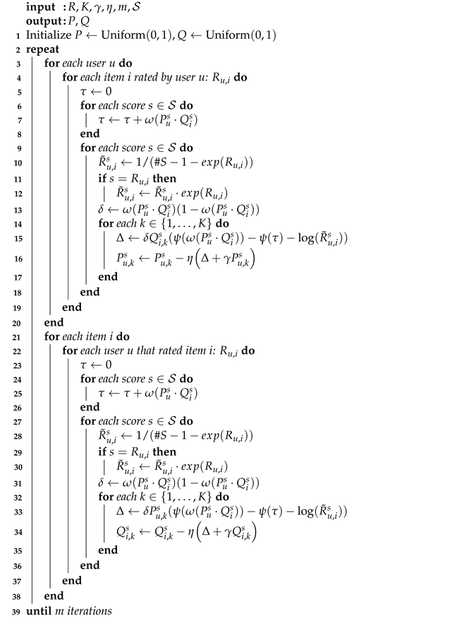
Algorithm 1 summarizes the fitting process of the DirMF model for $\omega =\frac{1}{1+e^{-x}}$ the genuine logistic function and ${\beta }_{u,i}=R_{u,i}$ to control the sharpness of the softmax function.

The algorithm requires as input the sparse rating matrix (R), the number of latent factors (K), the set of scores ($\mathcal{S}$), and the hyper-parameters that are required by gradient ascent optimization: learning rate ($\gamma$), regularization ($\eta$) and number of iterations (m) as inputs. Its outputs are the fitted latent factors: P contains the latent factors for each score s, user u and factor k, whereas Q contains the latent factors for each score s, item i and factor k. Note that both the user’s (lines 3–20) and item’s update loops (lines 21–38) may be executed in parallel for each user and item, respectively.

2.2. Prediction

Once the model has been trained, we have obtained a collection of users’ latent vectors $P_u^s$ as well as items’ latent vectors $Q_i^s$ for $s\in \mathcal{S}$. Given a new pair user–item $(u,i)$ to be predicted, the Dirichlet MF method assigns to it the D-dimensional continuous random vector ${\mathbf{R}}_{u,i}=({\mathbf{R}}_{u,i}^1,\dots ,{\mathbf{R}}_{u,i}^D)$ with parameters ${\rho }^s=\omega (P_u^s·Q_i^s)$. That is, it is the D-dimensional random vector supported on the standard simplex whose probability density function is given by (1):

$$f\left(x_1,\dots ,x_D|\omega (P_u·Q_i)\right)=\frac{1}{\mathrm{B}\left(\omega (P_u·Q_i)\right)}\prod _{s=1}^D{x}_s^{\omega (P_u^s·Q_i^s)-1}.$$

From this distribution, discrete random variables with supports on $\mathcal{S}$ can be sampled. These discrete probability distributions represent the probability that the user u would score item i with each of the possible ratings. However, observe that, in sharp contrast with other matrix factorization approaches, the output ${\mathbf{R}}_{u,i}$ here is not a discrete distribution, but a random variable that takes values in discrete probability distributions.

Several criteria can be used to obtain the predicted ratings. In this work, we shall follow an approach based on the law of large numbers. Indeed, if we sampled ${\mathbf{R}}_{u,i}$ a large number of times, the mean probability of the score $s\in \mathcal{S}$ would be the mean of the s-th component of the Dirichlet distribution with parameters ${\rho }^1=\omega (P_u^1·Q_i^1),\dots ,{\rho }^D=\omega (P_u^D·Q_i^D)$, which is the value:

$$\mathbb{E}\left({\mathbf{R}}_{u,i}^s\right)=\frac{\omega (P_u^s·Q_i^s)}{{\displaystyle \sum _{s\in \mathcal{S}}\omega (P_u^s·Q_i^s)}}.$$

These means are positive $\mathbb{E}\left({\mathbf{R}}_{u,i}^s\right)\ge 0$ and ${\sum }_s\mathbb{E}\left({\mathbf{R}}_{u,i}^s\right)=1$, so they give rise to a discrete robability distribution on $\mathcal{S}$. From it, we obtain two relevant data:

• The final prediction ${\widehat{R}}_{u,i}$, which is the mode of the aforementioned distribution, that is,

  $${\widehat{R}}_{u,i}={\mathrm{argmax}}_s\mathbb{E}\left({\mathbf{R}}_{u,i}^s\right).$$
• The reliability ${\varrho }_{u,i}$ in the prediction, which is the probability attained at the mode of the distribution, that is,

  $${\varrho }_{u,i}={\max }_s\mathbb{E}\left({\mathbf{R}}_{u,i}^s\right).$$

In this manner, fixed a threshold $0\le \vartheta \le 1$, we can crop the predictions so that we artificially set ${\widehat{R}}_{u,i}=•$ (no prediction is issued) if the reliability does not achieves the given threshold, that is, if ${\varrho }_{u,i}<\vartheta$. Otherwise, when ${\varrho }_{u,i}\ge \vartheta$, we keep, as the prediction ${\widehat{R}}_{u,i}$, the mode of the mean probability distribution.

Summarizing, the workflow associated to a cycle of training and exploitation phases of the DirMF model is as follows:

• Collect the rating matrix R of shape $N\times M$ with the known votes per user and item;
• Choose hyperparameters K (number of latent factors), $\gamma$ (learning rate), $\eta$ (regularization), m (number of iterations) and $\vartheta$ (reliability threshold, for the exploitation phase);
• Execute the training algorithm for DirMF (Algorithm 1) with the chosen hyperparameters. The output of the training is a collection of pairs of matrices $(P^s=(P_1^s,\dots ,P_N^s),Q^s=(Q_1^s,\dots ,Q_M^s))$ for each possible vote s;
• Given a new pair $(u,i)$ of an user $1\le u\le N$ and an item $1\le i\le M$ to be predicted, compute the quantities

  $$\mathbb{E}\left({\mathbf{R}}_{u,i}^s\right)=\frac{\omega (P_u^s·Q_i^s)}{{\displaystyle \sum _{s\in \mathcal{S}}\omega (P_u^s·Q_i^s)}},$$

  for each possible score s;
• The prediction ${\widehat{R}}_{u,i}$ is the vote $s_0$ for which $\mathbb{E}\left({\mathbf{R}}_{u,i}^{s_0}\right)$ is maximum. The reliability is the value ${\varrho }_{u,i}=\mathbb{E}\left({\mathbf{R}}_{u,i}^{s_0}\right)$.
• If ${\varrho }_{u,i}\ge \vartheta$, then return prediction ${\widehat{R}}_{u,i}$; otherwise return that no reliable prediction can be issued.

2.3. Computational Complexity

From the information of Algorithm 1, it is possible to analyze the complexity of the DirMF model in terms of time and space consumption.

Let us first focus on the spent time. From lines 3–4 and 21–22, we observe that, for each training epoch, the training algorithm must iterate over the set of known votes, let us denote it by $\Delta$. Now, the entry corresponding to each of the matrix factorizations must be updated, and there are $\left|\mathcal{S}\right|$ of them (lines 6, 9, 24 and 27). Finally, each updating operation requires to modify each of the entries of the hidden vectors for users and items, and there are K of them (lines 14 and 32). Notice that the updates only require standard arithmetic operations, which are performed in constant time. Hence, taking the total number of training steps, we obtain an exact time consumption of $O\left(\right|\Delta \left|\right|\mathcal{S}\left|Km\right)$.

To analyze how this quantity scales with the size of the dataset, we can estimate it further. Typically in real world datasets, the number of known values is a constant proportion (around 1–5%) of the total numbers of pairs (user, item), and there are $NM$ of these pairs. On the other hand, $\mathcal{S}$ uses to be a small set (of the order of 10 possible ratings) and m is a hyperparameter that is fixed independently of the number of entries of the dataset. Hence, the time complexity can be estimated by $O\left(NMK\right)$, that is, the time complexity increases linearly with the number of users and items in the dataset, as well as with the number of hidden factors.

Algorithm 1: DirMF model fitting algorithm fixing $\omega$ for the logistic function and shape parameters ${\beta }_{u,i}=R_{u,i}$.

With respect to space consumption, notice that all the operations can be conducted in-place, so no extra space is needed apart from the computed values. These values correspond to the $\left|\mathcal{S}\right|$ pairs of matrices $(P^s,Q^s)$ of the corresponding matrix factorization for the binary matrix $R^s$. Since each of these pairs has shape $N\times K$ and $M\times K$, we get a space complexity of $O\left(\right|\mathcal{S}\left|NM{K}^2\right)$. Again, since $\left|\mathcal{S}\right|$ is a fixed value independent of the size of the dataset, this complexity scales as $O\left(NM{K}^2\right)$, that is, linearly in the number of users and items and quadratically in the number of hidden factors.

2.4. Running Example

Here we describe a running example of the DirMF model using a synthetic dataset with three users and five items. For the sake of simplicity, the set of possible ratings is $\mathcal{S}=\left\{✔,✖\right\}$, that is, like and dislike. The original rating matrix used for this example can be checked in

Table 1. Rating matrix used in the running example. Rating values are: like ✔ and dislike ✖.

${\mathit{R}}_{\mathit{u},\mathit{i}}$	${\mathit{i}}_1$	${\mathit{i}}_2$	${\mathit{i}}_3$	${\mathit{i}}_4$	${\mathit{i}}_5$
$u_1$	✖		✔	✔
$u_2$	✔			✔	✖
$u_3$	✖	✔		✔

.

Given the ratings, we can build the softmax of every rating $R_{u,i}^s$ (i.e., like, dislike) according to Equation (2), as shown in

Table 2. Softmax-normalized ratings. Note that only known ratings are normalized.

${\mathit{R}}_{\mathit{u},\mathit{i}}^{✔}$	${\mathit{i}}_{\mathit{1}}$	${\mathit{i}}_{\mathit{2}}$	${\mathit{i}}_{\mathit{3}}$	${\mathit{i}}_{\mathit{4}}$	${\mathit{i}}_{\mathit{5}}$	${\mathit{R}}_{\mathit{u},\mathit{i}}^{✖}$	${\mathit{i}}_{\mathit{1}}$	${\mathit{i}}_{\mathit{2}}$	${\mathit{i}}_{\mathit{3}}$	${\mathit{i}}_{\mathit{4}}$	${\mathit{i}}_{\mathit{5}}$
$u_1$	0.27		0.73	0.73		$u_1$	0.73		0.27	0.27
$u_2$	0.73			0.73	0.27	$u_2$	0.27			0.27	0.73
$u_3$	0.27	0.73		0.73		$u_3$	0.73	0.27		0.27

.

The parameters of the model are the latent factors for both users and items for every possible rating: $P^{✔},P^{✖},Q^{✔},Q^{✖}$. For the sake of simplicity, we fixed the number of latent factors to $K=3$. The random initialization of the parameters for this running example is shown in

Table 3. Random initialization of $K=3$ latent factors for both users P and items Q.

${\mathit{P}}_{\mathit{u},\mathit{k}}^{✔}$	${\mathit{k}}_{\mathit{1}}$	${\mathit{k}}_{\mathit{2}}$	${\mathit{k}}_{\mathit{3}}$	${\mathit{P}}_{\mathit{u},\mathit{k}}^{✖}$	${\mathit{k}}_{\mathit{1}}$	${\mathit{k}}_{\mathit{2}}$	${\mathit{k}}_{\mathit{3}}$
$u_1$	0.06	0.04	0.58	$u_1$	0.73	0.85	0.88
$u_2$	0.78	0.04	0.66	$u_2$	0.95	0.23	0.53
$u_3$	0.40	0.77	0.36	$u_3$	0.90	0.87	0.75
${\mathit{Q}}_{\mathit{i},\mathit{k}}^{✔}$	${\mathit{k}}_{\mathit{1}}$	${\mathit{k}}_{\mathit{2}}$	${\mathit{k}}_{\mathit{3}}$	${\mathit{Q}}_{\mathit{i},\mathit{k}}^{✖}$	${\mathit{k}}_{\mathit{1}}$	${\mathit{k}}_{\mathit{2}}$	${\mathit{k}}_{\mathit{3}}$
$i_1$	0.89	0.84	0.54	$i_1$	0.14	0.95	0.46
$i_2$	0.06	0.42	0.84	$i_2$	0.96	0.66	0.77
$i_3$	0.84	0.35	0.91	$i_3$	0.13	0.75	0.25
$i_4$	0.83	0.93	0.19	$i_4$	0.26	0.33	0.51
$i_5$	0.08	0.31	0.14	$i_5$	0.43	0.69	0.84

.

The optimization of the parameters is performed by a gradient descent algorithm, so the update rules defined by Equations (4) and (5) are applied on each m iteration step. For instance, the update rule for the second latent factor $k_2$ of item $i_3$ and dislike rating (✖) is:

$$\Delta Q_{i_3,k_2}^{✖}=P_{u_1,k_2}^{✖}·{\omega }^{\prime }(P_{u_1}^{✖}·Q_{i_3}^{✖})\left[\psi \left(\omega (P_{u_1}^{✖}·Q_{i_3}^{✖})\right)-\psi \left(\sum _{s\in S}\omega \left(P_{u_1}^s·Q_{i_3}^s\right)\right)-log(R_{u_1,i_3}^{✖})\right],$$

hence we should update that hidden factor as follows:

$$Q_{i_3,k_2}^{✖}\leftarrow Q_{i_3,k_2}^{✖}-\gamma \left(\Delta Q_{i_3,k_2}^{✖}+\eta Q_{i_3,k_2}^{✖}\right),$$

with $\gamma$ and $\eta$ being the learning rate and regularization, respectively.

Table 4. Latent factors for both users P and items Q after one iteration.

${\mathit{P}}_{\mathit{u},\mathit{k}}^{✔}$	${\mathit{k}}_{\mathit{1}}$	${\mathit{k}}_{\mathit{2}}$	${\mathit{k}}_{\mathit{3}}$	${\mathit{P}}_{\mathit{u},\mathit{k}}^{✖}$	${\mathit{k}}_{\mathit{1}}$	${\mathit{k}}_{\mathit{2}}$	${\mathit{k}}_{\mathit{3}}$
$u_1$	0.10	0.08	0.59	$u_1$	0.72	0.84	0.87
$u_2$	0.79	0.06	0.67	$u_2$	0.94	0.22	0.52
$u_3$	0.41	0.78	0.37	$u_3$	0.89	0.85	0.73
${\mathit{Q}}_{\mathit{i},\mathit{k}}^{✔}$	${\mathit{k}}_{\mathit{1}}$	${\mathit{k}}_{\mathit{2}}$	${\mathit{k}}_{\mathit{3}}$	${\mathit{Q}}_{\mathit{i},\mathit{k}}^{✖}$	${\mathit{k}}_{\mathit{1}}$	${\mathit{k}}_{\mathit{2}}$	${\mathit{k}}_{\mathit{3}}$
$i_1$	0.90	0.85	0.56	$i_1$	0.12	0.93	0.44
$i_2$	0.08	0.42	0.85	$i_2$	0.95	0.66	0.77
$i_3$	0.84	0.35	0.91	$i_3$	0.13	0.75	0.25
$i_4$	0.83	0.93	0.21	$i_4$	0.26	0.32	0.51
$i_5$	0.09	0.33	0.15	$i_5$	0.42	0.68	0.83

contains the latent factors after one iteration using regularization $\eta =0.01$ and learning rate $\gamma =0.1$.

Predictions can be computed after the model has been trained by finding the score that maximizes the probability in the classification task. For instance, to determine user $u_2$’s rating of item $i_2$, ${\widehat{R}}_{u_2,i_2}$, we may compute the probability distribution of this rating as follows:

$$\begin{array}{cc}\hfill \mathbb{E}\left({\mathbf{R}}_{u_2,i_2}^{✖}\right)& =\frac{\omega (P_{u_2}^{✖}·Q_{i_2}^{✖})}{{\sum }_{s\in \mathcal{S}}\omega (P_{u_2}^s·Q_{i_2}^s)}=\frac{0.81}{0.81+0.66}=0.55,\hfill \\ \hfill \mathbb{E}\left({\mathbf{R}}_{u_2,i_2}^{✔}\right)& =\frac{\omega (P_{u_2}^{✔}·Q_{i_2}^{✔})}{{\sum }_{s\in \mathcal{S}}\omega (P_{u_2}^s·Q_{i_2}^s)}=\frac{0.66}{0.81+0.66}=0.45;\hfill \end{array}$$

then, the model selects the most likely outcome ${\widehat{R}}_{u_2,i_2}=✔$ with a reliability of ${\varrho }_{u_2,i_2}=0.55$.

3. Evaluation of Dirichlet Matrix Factorization

This section features a comprehensive description of the experiments conducted to assess the suggested model. The experimental setup, which defines the datasets, baselines and quality metrics used during the evaluation, is described in Section 3.1. Section 3.2 contains the experimental data as well as a comparison of the proposed method’s performance against the chosen baselines.

All experiments in this paper have been carried out using Collaborative Filtering for Java (CF4J) (https://github.com/ferortega/cf4j, accessed on 30 November 2021) [19]. The source code of all experiments analyzed in this work is publicly available on GitHub (https://github.com/KNODIS-Research-Group/DirMF, accessed on 30 November 2021).

3.1. Experimental Setup

The MovieLens [20], FilmTrust [21], MyAnimeList [22] and Netflix [23] datasets were used to conduct the experiment. These datasets were chosen to see how splitting the rating matrix into binary rating matrices with various discrete sets of possible scores affected the results. Both MovieLens and Netflix datasets comprise ratings ranging from one to five stars. FilmTrust ratings vary from 0.5 to 4.0 in half-step increments, while the MyAnimeList dataset has a score range of 1 to 10. Furthermore, all of these experiments were conducted using the benchmark version of these datasets, which is supplied in CF4J, to assure reproducibility.

Table 5. Datasets used in the experiments.

Dataset	No. Users	No. Items	No. Ratings	No. Test Ratings	Rating Scale
MovieLens1M	6040	3706	911,031	89,178	1 to 5
FilmTrust	1508	2071	32,675	2819	0.5 to 4.0
MyAnimeList	69,600	9927	5,788,207	549,027	1 to 10
Netflix Prize	480,189	17,770	99,945,049	535,458	1 to 5

summarizes the basic features of these datasets.

According to Section 1, all MF models in the literature can estimate a user’s rating prediction for an item, but only a few are able to offer the reliability of both their predictions and recommendations. Baselines were chosen to provide a diverse representation of all the known MF models. The selected baselines and their resulting outputs are:

• Bernoulli Matrix Factorization (BeMF) [18], which provides both prediction and recommendation reliability;
• PMF [10], which provides predictions but no reliability;
• GMF [11], which provides predictions only;
• NCF [11], which provides predictions but no reliability.

Several hyperparameters in both the specified baselines and our model must be tweaked. By executing a grid search optimization that minimizes the mean absolute prediction error, we evaluated the prediction error of baseline models with varied values of these hyperparameters. The hyperparameters derived by this optimization method for each baseline and dataset are listed in

Table 6. Baseline hyperparameters obtained by grid search optimization.

Method	MovieLens	FilmTrust	MyAnimeList	Netflix
PMF	$\mathrm{factors}=8$, $\gamma =0.01$, $\lambda =0.045$	$\mathrm{factors}=4$, $\gamma =0.015$, $\lambda =0.1$	$\mathrm{factors}=10$, $\gamma =0.005$, $\lambda =0.085$	$\mathrm{factors}=8$, $\gamma =0.01$, $\lambda =0.06$
NCF	$\mathrm{factors}=5$, $\mathrm{epochs}=10$	$\mathrm{factors}=5$, $\mathrm{epochs}=8$	$\mathrm{factors}=7$, $\mathrm{epochs}=15$	$\mathrm{factors}=6$, $\mathrm{epochs}=4$
GMF	$\mathrm{factors}=5$, $\mathrm{epochs}=10$	$\mathrm{factors}=5$, $\mathrm{epochs}=15$	$\mathrm{factors}=7$, $\mathrm{epochs}=20$	$\mathrm{factors}=5$, $\mathrm{epochs}=4$
BeMF	$\mathrm{factors}=2$, $\gamma =0.006$, $\lambda =0.16$, $m=100$	$\mathrm{factors}=2$, $\gamma =0.02$, $\lambda =0.06$, $m=75$	$\mathrm{factors}=4$, $\gamma =0.004$, $\lambda =0.1$, $m=100$	$\mathrm{factors}=6$, $\gamma =0.0006$, $\lambda =0.02$, $m=50$
DirMF	$\mathrm{factors}=6$, $\gamma =0.01$, $\eta =0.022$, $m=50$	$\mathrm{factors}=8$, $\gamma =0.015$, $\eta =0.09$, $m=100$	$\mathrm{factors}=10$, $\gamma =0.02$, $\eta =0.01$, $m=100$	$\mathrm{factors}=10$, $\gamma =0.02$, $\lambda =0.02$, $m=50$

.

Additionally, we set the DirMF method to work with the logistic activation function $\omega \left(x\right)={(1+e^{-x})}^{-1}$. As shape parameters for the softmax function we took ${\beta }_{u,i}=R_{u,i}$. Notice that this choice allows the system to straighten the most relevant votes (those with $R_{u,i}$ high) using a more spiky softmax function, compared to the less relevant votes (those with $R_{u,i}$ small) for which the softmax function used is flatter.

To assess the quality of the predictions and recommendations provided by a RS based on CF we define Mean Absolute Error (MAE) (Equation (6)) as the mean absolute difference between the test ratings ($R_{u,i}$) and their predictions (${\widehat{R}}_{u,i}$), and coverage (Equation (7)) as the proportion of test ratings that CF can predict (${\widehat{R}}_{u,i}\ne •$) with respect to the total number of test ratings. Here, $R^{\mathrm{test}}$ is the set of pairs $(u,i)$ of user u and item i in the test split of the dataset, and $\#R^{\mathrm{test}}$ denotes its cardinality.

$$\mathrm{MAE}=\frac{1}{\#R^{\mathrm{test}}}\sum _{\langle u,i\rangle \in R^{\mathrm{test}}}|R_{u,i}-{\widehat{R}}_{u,i}|.$$

(6)

$$\mathrm{coverage}=\frac{\#\{\langle u,i\rangle \in R^{\mathrm{test}}|{\widehat{R}}_{u,i}\ne •\}}{\#R^{\mathrm{test}}}.$$

(7)

Furthermore, two adapted quality measures emerge by fixing a number $n>0$ of top recommendations to consider: precision is defined as the averaged ratio of successful recommendations that are included in the top n recommendations for the user u, $T_u^n$, with respect to the size n of the recommendation list (Equation (8)); recall is the averaged proportion of successful recommendations included in the recommendation list of user u, $T_u^n$, with respect to the total number of test items that user u likes (Equation (9)).

$$\mathrm{precision}=\frac{1}{N}\sum _{u=1}^N\frac{\{i\in T_u^n|R_{u,i}\ge \theta \}}{\#T_u^n}.$$

(8)

$$\mathrm{recall}=\frac{1}{N}\sum _{u=1}^N\frac{\{i\in T_u^n|R_{u,i}\ge \theta \}}{\{i\in R_u^{\mathrm{test}}|R_{u,i}\ge \theta \}}.$$

(9)

Here, the variable u runs over the users of the dataset, N is the total number of users, $R_u^{\mathrm{test}}$ is the collection of items rated by user u in the test split and $\theta$ is a threshold to discern whether a user likes an item ($R_{u,i}\ge \theta$) or not ($R_{u,i}<\theta$).

3.2. Experimental Results

As mentioned above, we are able to tune the output of the DirMF model by filtering out less reliable predictions, hence decreasing the coverage of the model as some predictions cannot be recommended because the model does not have enough confidence to make them, but increasing the prediction accuracy at the same time. It is fair to believe that high-reliability predictions are more evident than low-reliability predictions. For instance, if a user gave The Lord of the Rings: The Fellowship of the Ring and The Lord of the Rings: The Two Towers favorable ratings, the model will have high confidence in the user’s positive interest in The Lord of the Rings: The Return of the King and will give this prediction a high reliability score. In contrast, the same algorithm will have less trust in the user’s interest in other fantasy films, such as The Princess Bride or Willow, and will give these predictions lower reliability scores.

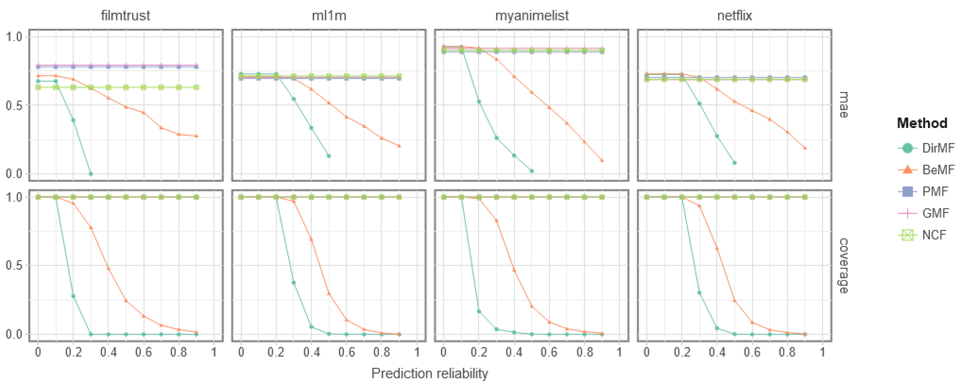
3.2.1. Mae vs. Coverage

Figure 2 shows the effect of using a reliability threshold on the quality of the predictions. The plots were created by filtering out any prediction with lower reliability than the x-axis reliability. Notice that only those models that output prediction reliabilities can filter their forecasts. For this reason, PMF, GMF and NCF are represented in the graphic as a horizontal line since varying the threshold do not affect their predictions.

To be precise, the plots of Figure 2 represent the evolution of the MAE and coverage quality measures, as specified in Equations (6) and (7). In this way, we compared the prediction error to the model’s predictability. As can be seen, there is a consistent trend within the plots, as unreliable predictions are filtered out, both the coverage and prediction error decrease. Furthermore, DirMF exhibits a more conservative behavior compared to BeMF, as shown by the sudden decrease in coverage which accompanies a similarly sudden decrease in MAE. This points out that the holistic interpretation of DirMF compared to BeMF allows it to extract subtle features of the data, which decreases its reliability in the prediction but also improves its ability to issue correct forecasts.

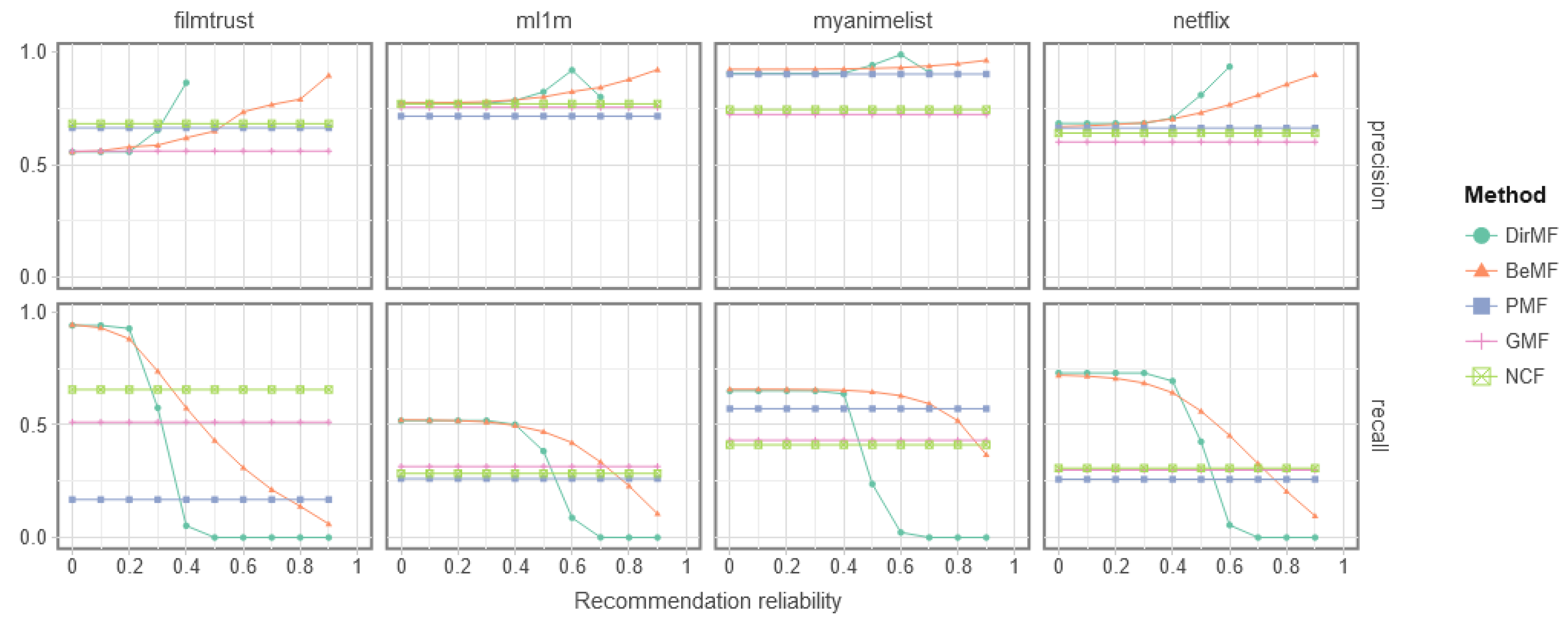
3.2.2. Recommendation Quality

To assess the recommendation quality, we calculated the precision (Equation (8)) and recall (Equation (9)) of the top ten recommendations ($n=10$) for each model. We set the threshold $\theta$ for determining which items attract a user based on his/her test ratings to $\theta =4$ for MovieLens and Netflix, $\theta =3.5$ for FilmTrust, and $\theta =7$ for MyAnimeList.

To create the recommendation lists predicted by each method, we have chosen the top 10 test items with the highest prediction (${\widehat{R}}_{u,i}$), omitting those with a prediction lower than $\theta$. Moreover, for those methods that also provide a reliability metric, we only considered those predictions with a reliability greater than or equal to the set reliability threshold $\vartheta$ (reliability ${\rho }_{u,i}\ge \vartheta$). Notice that the roles of $\vartheta$ and $\theta$ are distinct: the former is a threshold in desired reliability, whereas the latter is a threshold in predicted score.

These findings are presented in Figure 3. Again, the x-axis represents the reliability threshold $\vartheta$ below which predictions are filtered away. In this way, as we increase the threshold, for those methods that support reliability (DirMF and BeMF), the recall value falls while the precision value rises, as shown in that figure. Both our new DirMF approach and our previous BeMF model achieve better recall results than the other baselines when the prediction reliability is very low (between 0.4 and 0.6, depending on the dataset). Compared to BeMF, the recall of DirMF decreases more prematurely with respect to the reliability of the predictions, reinforcing the idea that the DirMF model is more conservative.

With respect to precision, it can be observed that DirMF and BeMF manage to improve the result obtained by the baselines, although each one achieves it with different levels of reliability indicating, once again, the more conservative approach of DirMF. In any case, DirMF manages to outperform not only BeMF, but all other baselines in absolute terms of precision.

3.2.3. Time and Space Complexity

We would like to finish this section with some words on the time and space complexity of the used algorithms. As computed in Section 2.3, DirMF has a time complexity of $O\left(NMK\right)$ and a space complexity of $O\left(NM{K}^2\right)$. These values are similar to the ones of PMF and BeMF, since both are based on a matrix factorization. Additionally, these bounds are smaller than the time and space complexity of the neural network-based models GMF and NCF. Indeed, these methods, apart from computing a matrix factorization, also need to compute the weights of the inner product (GMF) or even those of a whole neural network (NCF) used to combine the hidden factors.

In this way, DirMF is as efficient in terms of time and space as the existing MF methods, and even more efficient with respect to those that apply deep learning techniques.

4. Conclusions

The DirMF model, which is an MF-based CF method that yields not just predictions for things that have not been evaluated by users, but also the reliability of these predictions, is provided in this study. By approaching the recommendation process as a classification problem rather than a regression one, this result is accomplished. The DirMF model’s output pair of both prediction and reliability allows us to calibrate it to achieve the correct balance between the quality and quantity of the predictions (i.e., to reduce the prediction error by limiting the model’s coverage).

DirMF builds on the progress made with our previous model, BeMF [18], where the use of other probability distributions as underlying assumptions for the MF method was identified as future work worth pursuing. This is exactly what has been done, using a Dirichlet probability distribution as the underlying assumption instead of Bernoulli random variables, which assume independence between the ratings.

Experimental results show that DirMF and BeMF achieve better recall results than the baselines when the prediction reliability is very low (between 0.4 and 0.6, depending on the dataset), although the recall of the former decreases more quickly with respect to the reliability of the predictions. Regarding precision, again, our model DirMF achieves better values than those obtained by the baselines, improving BeMF’s results on some datasets. According to those results, we can conclude that our model DirMF is more conservative with its predictions than BeMF. This means that DirMF tends to be more prudent when issuing predictions, but those emitted have a much larger chance of being accurate. In this manner, the quality of the DirMF predictions with large thresholds is better that for BeMF, at the cost of issuing less predictions. This behavior is desirable in those scenarios in which failure is highly penalized, like customers with a small chance of re-entering the system, medical predictions, or critical industrial forecasting.

It is worth mentioning that BeMF and DirMF are two methods that, by design, incorporate reliability at the core of the training process of the matrix factorization algorithm. For this reason, BeMF and DirMF are able to outperform other methods, which do not intrinsically treat reliability, in terms of accuracy of predictions. The probabilistic assumption that rating is a process that must be modeled as several binary classification problems (as done by BeMF and DirMF), instead of a single regression problem (as done by PMF, GMF, NCF) seems to be much more accurate in most scenarios, leading to better predictions. This trend becomes even more prominent when we set a reliability threshold $\vartheta$: with this threshold, BeMF and DirMF are able to filter out non-reliable prediction, which are those that, more likely, will be misclassified; whereas PMF, GMF and NCF cannot make use of this capability, since they do not implement a native management of reliability.

As a future work, we suggest examining the quality of our model in terms other than accuracy, that is, novelty, diversity and discovery. Similarly, we advise testing the model’s stability against shilling attacks, which are used to discredit or promote some items over the rest. Furthermore, our model might be expanded to include both social and content information to increase the quality of the predictions.