Article

Resolving Data Sparsity via Aggregating Graph-Based User–App–Location Association for Location Recommendations

1
School of Electronics and Information Technology, Sun Yat-sen University, Guangzhou 510006, China
2
Key Laboratory of Industrial Internet and Big Data, China National Light Industry, Beijing Technology and Business University, Beijing 100048, China
*
Author to whom correspondence should be addressed.
Appl. Sci. 2022, 12(14), 6882; https://doi.org/10.3390/app12146882
Submission received: 6 June 2022 / Revised: 4 July 2022 / Accepted: 4 July 2022 / Published: 7 July 2022

Abstract

:
Personalized location recommendations aim to recommend places that users want to visit, which can save their decision-making time in daily life. However, the recommending task faces a serious data sparsity problem because users have only visited a small part of total places in a city. This problem directly leads to the difficulty in learning latent representations of users and locations. In order to tackle the data sparsity problem and make better recommendations, users’ app usage records in different locations are introduced to compensated for both users’ interests and locations’ characteristics in this paper. An attributed graph-based representation model is proposed to dig out user–app–location associations with high-order features aggregated. Extensive experiments prove that better representations of users and locations are obtained by our proposed model, thus it greatly improves location recommendation performances compared with the state-of-art methods. For example, our model achieves 13.20%, 10.1%, and 9.44% higher performance than the state-of-art (SOTA) models in T o p 3 H i t r a t e , T o p 3 A c c u r a c y , and n D C G 3 , respectively, in the Telecom dataset. In the TalkingData dataset, our model achieves 9.34%, 13.35%, and 8.56% better performance than the SOTA models in T o p 2 H i t r a t e , T o p 2 A c c u r a c y , and n D C G 2 , respectively. Furthermore, numerical results demonstrate that our model can effectively alleviate the data sparsity problem in recommendation systems.

1. Introduction

With the improvements of living standards, people are more willing to travel and enjoy themselves in places they have not been to. Thus, personalized location-based social networks (LBSNs) and recommendation services emerge and have a rapid development, such as the famous review website Yelp, travel platform Mafengwo, etc. [1]. How to recommend yet-unvisited locations that meet the users’ interests has become a popular research topic. Many scholars and application developers invest time and efforts in this task for urban development and the improvement of users’ experience. For example, some researchers want to increase the exposure of less popular locations and promote the economy of a city [2,3]. More and more useful functions are developed in industrial applications that enable users to save decision-making time and avoid travel crowds, and have reward of more pleasant and satisfactory travel experiences. Nowadays, the widespread usage of electronic footprints in mobile positioning technology, such as check-in data in social networks, call detail records or GPS coordinates recorded by mobile phones, enable the location-based services to develop fast. Researchers can exploit the interests of users and improve their personalized location recommender system [4].
To improve recommendation performances, it is significant to understand and exploit user-location latent associations. Recently, many methods aim to explore the implicit representations of users and locations from user-location interactions. For example, location recommendation frameworks GeoMF [5] and GeoMF++ [6] are based on matrix factorization, which introduces geographic features into matrix construction and obtains decomposed geographic features. Various neural networks are also proposed to discover non-linear relationships between users and locations. Zhong et al. [7] propose a points of interests (POIs) recommendation model which uses long short-term memory (LSTM) to model check-in data. It also takes the advantage of the multi-layer perceptron (MLP) to integrate social influence and location popularity. A spatio-temporal attention network (STAN) with the dual attention architecture is proposed to predict user’s next position [8]. Ameen et al. [9] use a combination of convolutional neural network and matrix factorization to obtain latent visiting behaviors. Although these models learn latent embeddings through user-place interactions, they cannot explicitly use the relationships of user–user and place–place, which obviously limits the representation ability.
In recent years, due to the advantages of graphs in explicitly presenting entities’ interactive relationships, graph-based recommendation algorithms have drawn widespread attention [10,11]. Explicit interaction structures, such as the adjacency between locations, or friendship between users, can be easily expressed under a graph structure. Now, graph representation learning are widely used to improve recommendations [12,13], and pursuing the interpretability in recommender system [14]. Nevertheless, there are no research works using graph learning network to solve data sparsity that rooted in recommender system. Therefore, in order to effectively integrate the interactive associations among entities, i.e., users and locations, we propose a graph-based representation model to dig out implicit embedding features of users and locations, respectively, and tackle the data sparsity problem.
However, it is not easy to achieve accurate recommending results not only by model ability, but also for serious data sparsity [15,16], which deeply roots in recommendation systems. To make matters worse, location recommendations have serious temporal and spatial dependence. Compared to millions of locations marked in maps, a user usually leaves footprints only in very few places, actually. For example, the density of user–location check-in data is less than 0.1%, as the research [17] shows. Therefore, it is difficult to learn users’ location preferences and location characteristics from too few interaction behaviors, let alone to obtain high-accuracy location recommendation results. In order to solve the data sparsity problem, a common and useful practice is introducing external sources, in which user interests or location features can be filled up [18,19,20]. For example, we can extract the auxiliary information such as users’ age, gender, social relationship, POIs around locations [21,22,23] to solve data sparsity problem. However, the acquisition of these additional sources is very difficult to collect for the privacy preservation of users.
Although these research works made contributions on enhancing representations [24,25] or tackling data sparsity [26,27], they did not solve the two problems simultaneously. In this paper, we propose a graph-based representation model that not only increases recommendation accuracy but also tackles the data sparsity problem. To be specific, we introduce app usage records into the graph-based model, which can obtain high-order associations of user–location–app, i.e., user–location, user–app, location–app etc., contributing a lot to recommendation quality even under severe data sparsity.
The rest of this paper is organized as follows. Section 2 reviews the related work about location recommendations and the data sparsity problem. Section 3 introduces the datasets and analyses the feasibility of location recommendations with app usage data. Section 4 describes our recommender framework in detail. Section 5 evaluates its performances and discusses the experimental results, followed by the conclusion in Section 6.

2. Related Work

Personalized location recommendations have drawn wide attention in academia and industry recently. However, this task still faces the data sparsity problem that is rooted in recommendation systems. The relevant works in personalized location recommendations and solutions of data sparsity are reviewed, respectively, in detail.

2.1. Personalized Location Recommendations

Personalized location recommendations aim to recommend locations that users have not visited but may be interested in, such as natural attractions, shopping malls, etc. In order to improve recommendation performances, it is important to effectively dig out user–location latent associations. Many researchers have made contributions on this task, aiming to explore the implicit representations of user interests and location characteristics from their interactions. There are several strands of classical models for location recommendations. The first strand of model are random models, which can capture macroscopic features mathematically, but they are not accurate, such as Markov chains [28] and Bayesian personalized ranking models [29,30], support vector machines [31]. The second strand of models are collaborative filtering models based on machine learning, which develop fast for their abilities in obtaining interactive features [5,6,32,33,34]. For example, location recommendation frameworks GeoMF and GeoMF++ introduce the geographic features into matrix factorization, which obtains implicit geographic embeddings to improve location recommendations [5,6]. Nowadays, with the continuous expansion of data scale, deep learning-based models become the third strand of models used in the location recommendations, enhancing the representation ability of entities and hence improving their performances. Qi et al. [35] use LSTM to learn the long-term interests of users’ travel behavior, and provide users with personalized travel location recommendations. Zhao et al. [36] propose a location recommendation model based on federated learning. It trains two neural networks to realize location recommendations at the same time, by fully exploring users’ implicit interests in location-visited sequences in the short term and long term. Based on GAN (generative adversarial network), Zhou et al. [37] propose an adversarial location recommendation model, which contains two antibodies to obtain user embeddings to recommend proper locations. Nevertheless, the aforementioned methods are still limited to obtaining optimal recommendation results because they cannot use explicit connections between entities, i.e., the similarity between users and the adjacency between locations.
Recently, graph-based models are widely applied in recommender systems for their great abilities in aggregating high-order features and capturing implicit characteristics [10,11]. Merging the idea of neural network and the representation ability of graph structure, graph neural network (GNN) is a typical application. Among various kinds of GNNs, graph convolutional neural network [38] (GCN) well outperforms the others due to its efficient integration on user–item interactions by graph convolution, which enhances the feature representation capability of recommender model.
There are many research works applying GNNs into location recommendations, proving that it can works better in the recommending task due to its strong information aggregation and representation ability. Wang et al. [39] propose neural graph collaborative filtering (NGCF), which uses GCN to obtain decomposed embeddings of users and items, and improves recommending results compared with traditional matrix factorization. In [40], Chen et al. propose a subgraph-based graph embedding method, SgWalk, to capture contextual relationships based on user subgraph. Xu et al. [41] propose Venue2Vec model, which incorporates temporal–spatial context and semantic information into fine-grained location prediction of users. Zhong et al. [42] propose a location recommend framework with hybrid graph convolutional networks. Compared with collaborative filtering-based and other deep learning-based recommendation methods, GNNs can well learn the representations of users and items. However, these work ignore the node attributes and do not solve the data sparsity problem. Thus we propose a graph-based representation model for personalized location recommendations, which constructs an attributed bipartite graph from user–app–location associations and utilize the graph convolution method to capture high-order features.

2.2. Data Sparsity Solutions

Obviously, it is important to exploit the users’ and locations’ embeddings well, which is not only limited by the models’ representation ability, but is also influenced by the sparsity of user-location interactions [26]. A user usually visits few locations in a city during their daily routine. However, if they have a short travel time, the location visiting will become more random, meaning it is hard to make recommendations. The sparse interactions and random behaviors inspire us to overcome the data sparsity and acquire more information, whether explicit or implicit, to improve recommending results. To overcome the extreme sparsity of user–location interactions, the canonical method is to introduce external sources as auxiliary information to explore latent user interests or location features. In [18], users’ information are supplied, such as age, gender, etc., which believes that users with similar attributes may have similar location preferences. Social relationships such as Facebook friendship [19,43] are also considered as an important role in recommendations owing to the fact that people in an intimate relationship often share interests and travel together. However, these information about users are too private to collect. In order to extract the location characteristics, POIs are often considered. Yu et al. [20] use POIs categories and geographic proximity to improving location recommendations under data sparsity, because POIs often reveal the similarity between two places.
In fact, many studies [44,45] have shown that app usage records in telecommunications can reflect users’ personal interests, because app usage patterns of different users are quite different. Furthermore, there is also a strong correlation between the users’ app usage and location attributes [46,47]. For example, Yu et al. [47] find that the usage frequency of music apps in sport venues is higher, and educational apps are used more frequently in the school. Tu et al. [23] introduce app data into location recommendations and prove that the cold-start problem can be mitigated a lot, but they do not discuss whether it is useful in solving data sparsity. Therefore, we consider utilizing app usage data because it can not only indicate user interests but also reflect functional attributes of locations, which provides an opportunity to learn user preferences and location features with less information collected. To our best knowledge, this is the first time that app usage records have been utilized to solve data sparsity in personalized location recommendations, and our experimental results show that this method is quite effective and feasible.

3. Datasets and Analyses

We conduct experiments on two real-world datasets based on telecommunication data. Details and analysis about the datasets are introduced in this section.

3.1. Datasets

Telecom Dataset : This dataset is collected by one of the biggest telecom operator in Shanghai, China [47]. It contains app usage records of mobile users in Shanghai. Each record contains: anonymous user ID (Identity Document), time, base station ID, its latitude and longitude coordinates, and current app ID. This dataset contains 9.4 billion records generated by 1.37 million users from 20 to 26 April 2016, and covers the 2000 most popular apps in the App Store and Google Play. In the dataset, the records of 10,000 users who visited more than 10 locations and used more than 5 apps in each location are selected. Finally we obtain this dataset, called Telecom dataset, with over 40 million records, containing 11,584 locations and 1327 apps.
TalkingData: This dataset is collected by TalkingData SDK (Software Development Kit, which is integrated in mobile applications) and published on the Kaggle website [48]. Each record includes anonymous device ID, time, latitude, longitude, and app ID, which reflects users’ app usage behavior. The dataset is pre-processed as follows. First, the coverage area is divided into grids of 1 km × 1 km, and the latitude and longitude coordinates are converted into grid IDs. Second, the 40,000 densest area in a square and users with more than 30 records are selected. Moreover, the locations and apps accessed by less than five users are filtered out in order to reduce noise in the dataset. In the end, an app usage dataset with 256 users, 689 apps and 439 locations is obtained.
Table 1 summarizes the key information of Telecom and TalkingData datasets.

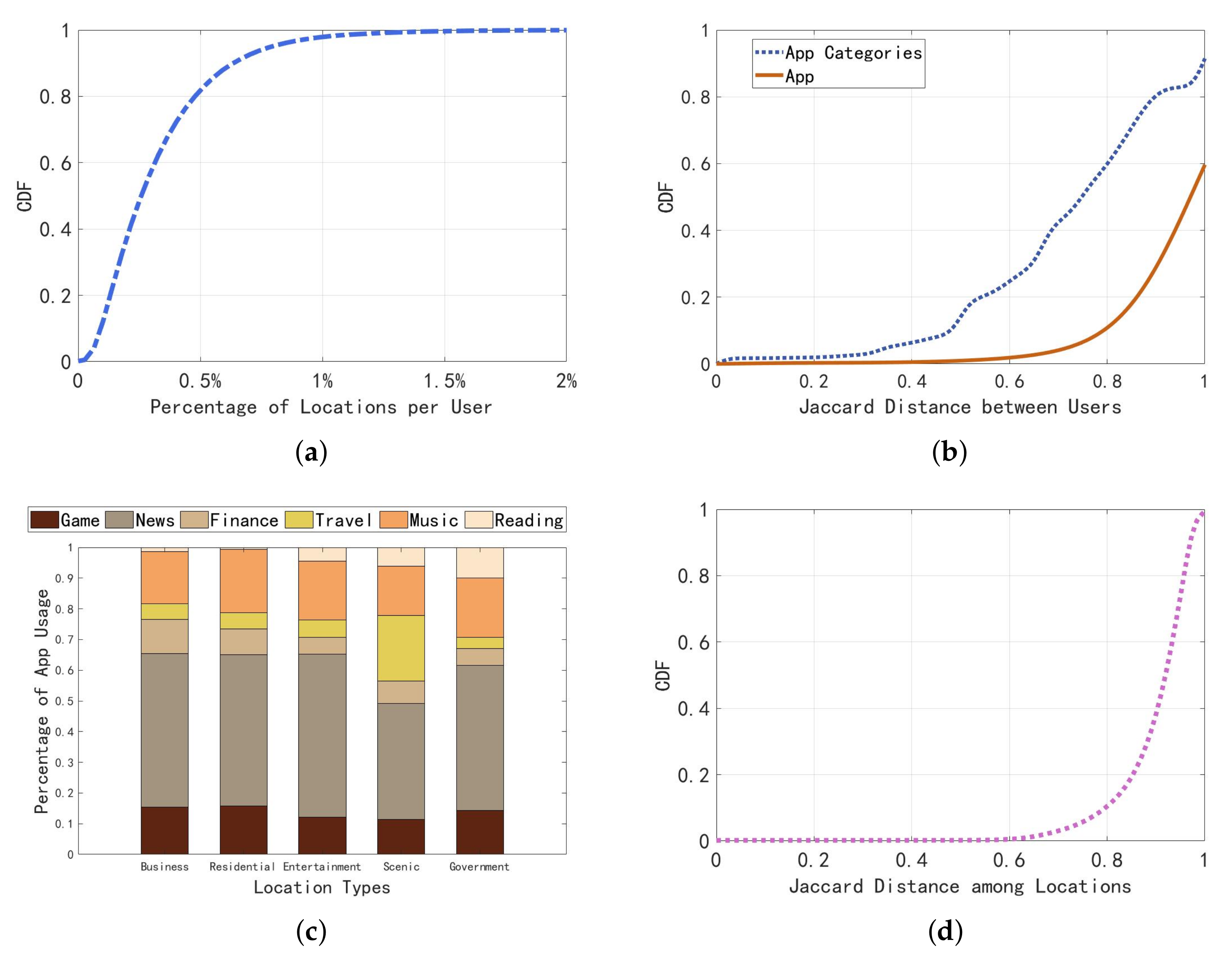
3.2. Analyses of User–Location–App Associations

We first integrate the basic statistics of the Telecom dataset. We calculate the percentage of all locations visited by each user in all locations, and plot the Cumulative Distribution Function (CDF) curve in Figure 1a. It demonstrates that the locations visited by most users only account for less than 1% of all locations, and even 80% of users have only visited less than 0.5% of all locations. In fact, we can see from Figure 1a that users have visited only 2% of locations at most. On TalkingData dataset, the sparsity is also severe, in which the places for users ever visited are less than 1% in total. Compared to all available locations, there are very few places visited by each user, thus it is difficult to provide accurate recommendations with insufficient information.
In order to overcome the above challenges, we find it feasible to use app usage patterns as attributes of users and locations after analyzing the characteristics of app usage in different users and locations. To be specific, we use Jaccard distance to measure the similarity between users from app usage frequencies and app categories, respectively. The Jaccard distance between user i and user j on app usage frequencies is denoted as J i j A :
J i j A = 1 S i A S j A S i A S j A , i , j = 1 , , N U ,
where S i A and S j A are the sets of apps used by user i and user j, respectively. N U is user number. The Jaccard distance between user i and user j on app usage frequencies is denoted as J i j C :
J i j C = 1 S i C S j C S i C S j C , i , j = 1 , , N U ,
where S i C and S j C are the sets of apps categories used by user i and user j, respectively. Then we plot CDFs of these two Jaccard lines as Figure 1b shows. It can be seen from the figure that there are differences in app usage behaviors of users. App usage data can also reflect the location characteristics to a large extent. As the Figure 1c shows, app usage behavior in different locations are quite different, which indicates that we can infer users’ personal interests from their app usage records. We also calculate the Jaccard distance between locations based on Telecom dataset. Assuming that the app appearing in location i and location j are, respectively, S i L and S j L . N L is the location number. The Jaccard distance J i j L between two locations is as follows
J i j L = 1 S i L S j L S i L S j L , i , j = 1 , , N L .
Then the CDF of Jaccard distance between all locations is shown in the Figure 1d, which shows that the Jaccard distance exceeds 0.8 in 90% location pairs, so that we can use app records to study different users’ different behavior patterns.
As we analyze above, the Telecom and TalkingData dataset are both in extreme data sparsity. Thus, we make three simple hypotheses as follows:
Hypothesis (H1).
Users’ interests are associated with their app usage behaviors.
Hypothesis (H2).
Locations’ characteristics are associated with app usage on them.
Hypothesis (H3).
Users’ interests are associated with locations characteristics and can be associated with app usage records.
To achieve effective information aggregation and representation learning, we propose a representation model via a graph convolutional network to effectively aggregate user–app–location associations from the attributed graph.

4. Methodology

4.1. Problem Preliminaries

The interactions between users and locations can be represented as a bipartite graph G = ( V , E , X ) . V stands for user and location nodes, E stands for undirect edges weighted by visit frequencies, and X stands for node attributes weighted by app usage frequencies. Then we aim to train a representation model f, which maps G into user representation U and location representation L . Then, given an user’s location visiting history ( u , L u ) , our model will first find the corresponding representation vectors, u and L u . Ranking score matrix R u ^ will be calculated by u · L u . Then the ranking score will be sorted and choose the Top-N list as we set. Finally, we evaluate the Top-N list and L u .

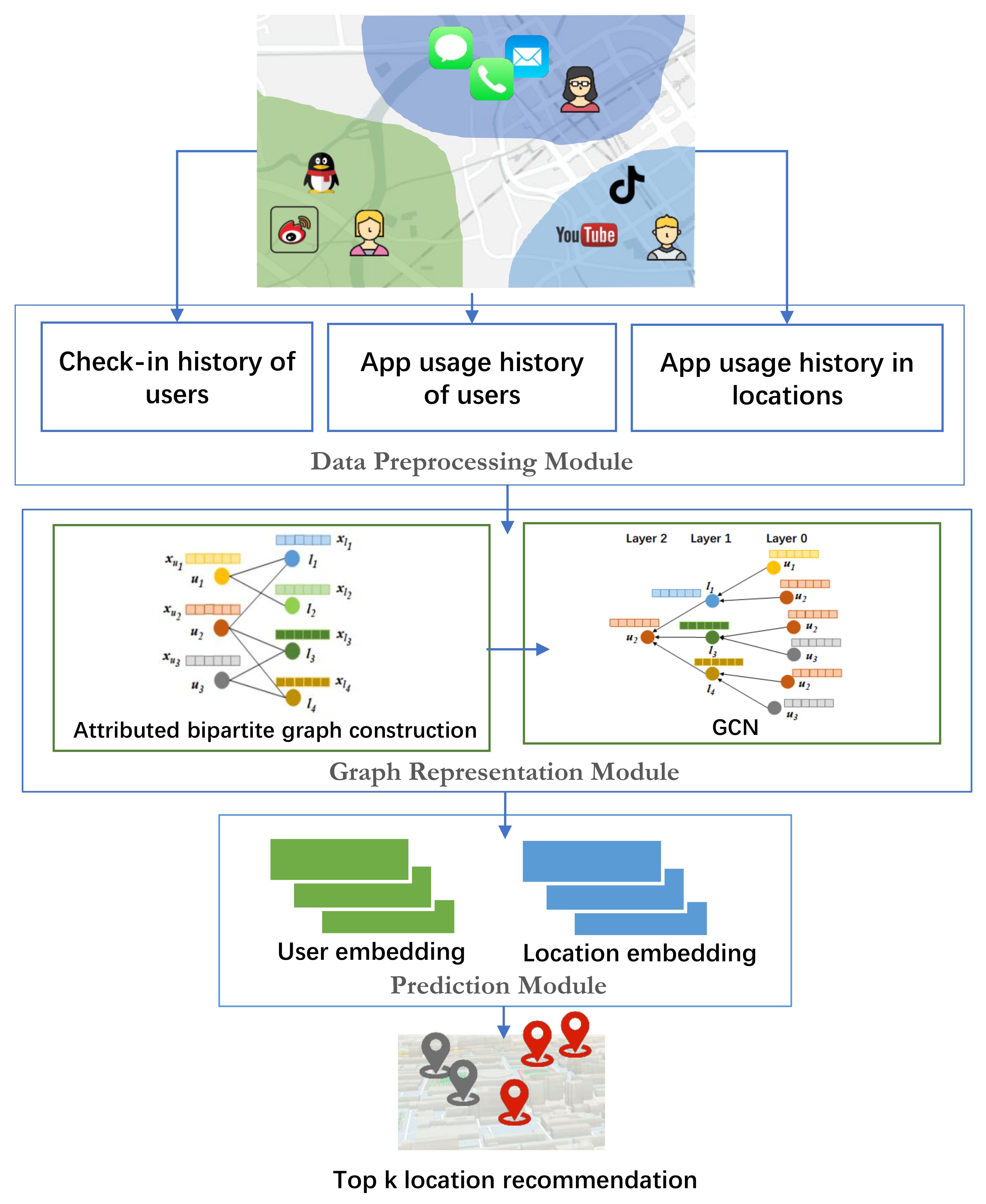
4.2. Framework of Proposed Recommendation Model

As Figure 2 shows, the proposed model contains three main modules: Preprocessing Module, R e p r e s e n t a t i o n M o d u l e , and P r e d i c t i o n M o d u l e . In the P r e p r o c e s s i n g M o d u l e , user–location, user–app and app–location interactions are obtained. An undirected bipartite graph G then is constructed with node attributes attached. Then the graph G is sent to R e p r e s e n t a t i o n M o d u l e . Latent preferences of users and locations are learned via the representation model based on graph convolution. Finally the P r e d i c t i o n M o d u l e generates the recommending locations for each user, and evaluations are conducted to ensure its effectiveness.

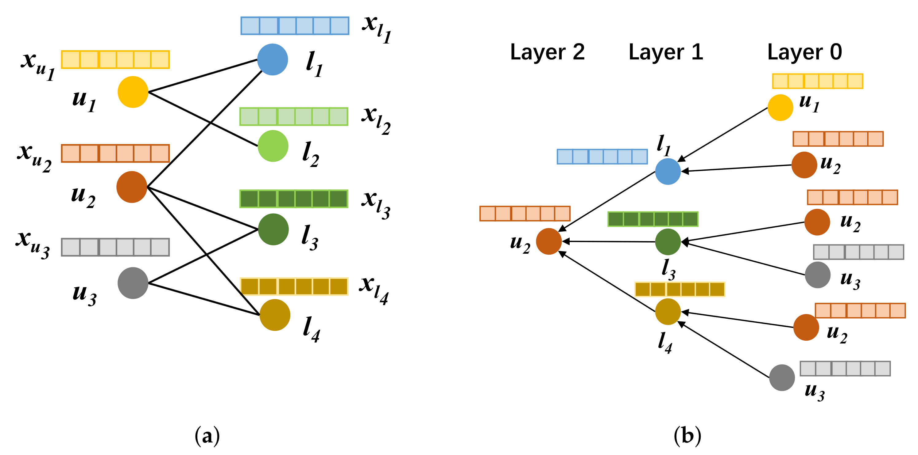
4.3. Generation of Attributed Bipartite Graph

We first extract the user–location interactive behavior from app records. Subsequently, user and location attributes based on app usage behavior are calculated as supplementary information. Then, an user–location attributed bipartite graph is constructed as the input of the representation model.
Specifically, the usage frequency of different apps is taken as users’ app preferences. We use the maximum normalization to constrain the values. User u’s app preference x u can be denoted as
x u = < c u a M UA > a = 1 N A ,
where c u a represents the frequency of user u using app a. M UA is the maximum value of usage frequencies among all apps, and N A is the total number of apps.
Similarly, the usage preference of app in each location l is extracted as
x l = < c l a M LA > a = 1 N A ,
where c l a represents the total frequency of app a used in the location l. M LA is the maximum frequency.
Based on the extracted features, a bipartite graph G with node attributes is constructed. Users and locations are both set as nodes. Graph edges are established based on the interactive relationship between users and locations. Since there is no direction for visiting interactions, an undirected graph is built. In order to distinguish the different visits on various locations, we take users’ preferences of different locations as the edge weights. To be specific, user u’s preference J u l of the location l is
J u l = c u l M UL ,
where c u l represents the visiting frequency of user u to location l. M UL is the maximum value among all users’ visits. In addition, each node also has its own attributes as we mentioned above. The attributes of user u is x u , and the attributes of the location l is x l . Then the attributed graph G is contructed. The schematic diagram of G is shown in Figure 3a.
After constructing the bipartite graph with node attributes, an attributed-graph representation model via graph convolution network is proposed to obtain representations of nodes.

4.4. Representation Model Construction

The high-order feature aggregations and transfer principle of graph convolutional neural network are as follows. The information aggregation process of two-layer GCN is shown in Figure 3b. Specifically, we take the user node u 2 in the Figure 3a as an example. First, it finds the locations l 1 , l 3 , and l 4 that user u 2 has directly interacted with. Then, according to the graph structure, it finds the users who have interacted with these locations, respectively, i.e., l 1 -( u 1 , u 2 ), l 3 -( u 2 , u 3 ), l 4 -( u 2 , u 3 ). Starting from the 0th layer, the users’ node characteristics are transferred to location nodes in the 1st layer with theirs characteristics aggregated, which helps to generate high-order features of the locations. After that, new location features are transferred to the user node u 2 in the 2nd layer and aggregated with the user’s own feature x u 2 , generating new feature of user u 2 . In this way, the key information associated with the target user is gathered layer-by-layer, capturing the user’s implicit interests as well as the location characteristics.
In our proposed model, we construct the graph G = ( V , E , X ) as mentioned above, where V is the set of nodes in the graph, including user nodes and location nodes. E is the set of graph edges. X is the node’s attribute matrix. Each row of X represents the latent attributes of a node. The attribute matrix of users is X u and the attribute matrix of locations is X l , then the nodes’ attribute matrix X of the graph G can be written as:
X = X u X l .
Suppose the interaction matrix between users and locations is F R N U × N L , where F u l stands for the user u’s preferences for location l, then the adjacency matrix A of the graph G is
A = F 0 0 F T .
Denote the layer number of attributed graph convolutional network as k, then the principle of information aggregation for each node in the kth layer of our model is
θ u ( k ) = f θ u ( k 1 ) , θ v ( k 1 ) v N ( u ) = σ v N ( u ) u 1 d u d v θ v ( k 1 ) W k ,
where θ u ( k ) stands for the representation vector of node u in the kth layer. N ( u ) is the set of neighbor nodes of user u, d u , and d v stand for the degree of node u and node v, respectively. σ is activation function, and we use R e L U function here. W k is the weight matrix of kth layer. The initial representation of each node θ v ( 0 ) is its attribute vector x v . It can be seen from the (9) that high-order features of each node is obtained by the aggregation of attributes from its neighbors from the lower layer and itself.
Suppose Θ ( k ) = θ 1 ( k ) , θ 2 ( k ) , , θ | V | ( k ) , then we rewrite the input of model as
Θ ( 0 ) = X .
Then (9) is rewritten as:
Θ ( k ) = σ D ˜ 1 2 A ˜ D ˜ 1 2 Θ ( k 1 ) W ( k ) ,
where A ˜ = A + I , I is identity matrix. D ˜ is diagonal matrix, D i i = j A ˜ i j . In our research, the activation function will not be applied in kth layer [49].
With node attributes disseminated and aggregated by the network, the user representation vector U , U R N U × H and the location representation L , L R N L × H are obtained. Among them, H is the dimension of the representation vector, N U is the number of users, and N L is the number of locations.
Θ ( K ) = U L ,
where Θ is representation matrix of users U and locations L, U is the users’ representations, and L is the locations’ representations. Θ ( K ) R N U + N L × H , U R N U × H , L R N L × H .
The recommendations are based on the output of our model, the user representation U and the location representation L . We take the idea of collaborative filtering of matrix decomposition that the interested score of each user u to location l ¯ where they have not visited before is represented by the inner product of U and L . The formula is
f ^ u l ¯ = U u T L l ¯ .
Then according to the interesting score f ^ u l ¯ , the top-k locations are selected as recommended locations for users.

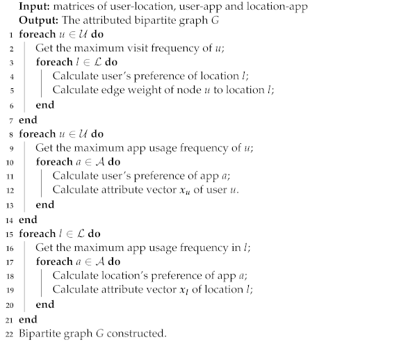
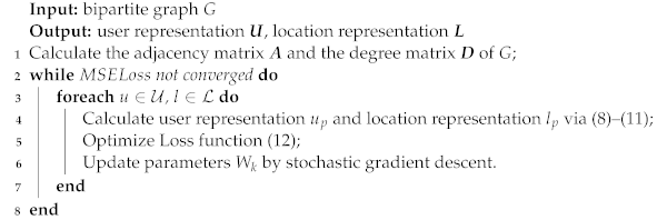
4.5. Graph Generation and Location Recommendation Algorithms

The modeling and training process of our attributed graph-based model are shown in this section. The construction of attributed bipartite graph is shown in Algorithm 1. The training process of the attributed-GCN is described in Algorithm 2. When training our model, we use Mean Squared Error (MSELoss) and Bayesian Personalized Ranking (BPRLoss) as loss functions and compare their performances [50]. The formula of MSELoss is
L m s e = 1 I F 0 I F F U L 2 2
where F is the interaction matrix between users and locations. I F is the identity matrix of F . If F i j 0 , then each element of the corresponding position in I F is 1 otherwise 0. “∘” means the dot product. · F 2 stands for 2 norm of vectors.
BPRLoss considers that positive samples might rank higher than negative samples. In our model, positive samples means the locations that user u have visited. The formula of BPRLoss is
L b p r = ( u , l i , l j ) S l n σ ( x ^ u l i x ^ u l j ) + λ θ Θ 2 2
where ( u , l i , l j ) means user–location pair, l i means positive sample that user has visited l j means negative sample. x ^ u l i means user u’s rating score on location l i , x ^ u l j means user u’s rating score on location l j , x ^ u l i = u · l i , x ^ u l j = u · l j . S means training samples set. σ ( · ) means sigmoid function. Θ means model parameters and λ θ means regularization parameters.
Algorithm 1: Constructing attributed bipartite graph
Applsci 12 06882 i001
Algorithm 2: Training process of our model
Applsci 12 06882 i002

5. Experiments and Evaluation

In order to evaluate the performances of our proposed model, extensive experiments are conducted on two real-world datasets.

5.1. Experimental Setting

5.1.1. Metrics

We adopt three prevalent metrics in recommender systems, i.e., TopK Hitrate, TopK Accuracy, and n D C G K to evaluate the recommending performances. We use different @ N values to evaluate two diffierent datasets because the number of samples in TalkingData is significantly smaller than that of Telecom Data.
T o p K H i t r a t e measures the successful proportion of users whose top-k recommended locations are predicted correctly for at least one location that hits the ground truth. The formula is expressed as follows.
T o p K H i t r a t e = i = 1 N ( | L i p L i t | 1 ) N ,
where L i p denotes the list of top-k recommended locations by the ith user in the test set. L i t denotes the K locations that are most frequently visited by the user u i , for each user u i U . N is the number of users in test set.
T o p K A c c u r a c y is used to measure the prediction accuracy on the top-k predictions of all users. The formula is
T o p K A c c u r a c y = i = 1 N ( | L i p L i t | / K ) N .
n D C G K (Normalized Discounted Cumulative Gain) is commonly used to measure the ranking quality of the top-k predicted results. The computation is expressed as follows
n D C G K = D C G K I D C G K = i = 1 N j = 1 K r e l j p ( i ) / l o g 2 ( j + 1 ) N j = 1 K r e l j t ( i ) / l o g 2 ( j + 1 ) ,
where r e l k p represents the prediction of the kth app’s usage frequency of the ith user in the jth place, and r e l k t represents the corresponding groundtruth. Higher value of n D C G K means better ranking quality.

5.1.2. Baselines

We compare the performances of our model with several state-of-art methods in personalized location recommender systems.
SVD-MFN [51]: Singular Value Decomposition with Multi-Factor Neighborhood (SVD-MFN) takes a variety of factors into consideration so as to better predict the users’ preferences for items. It aims to recommend the most similar items according to historical interactions. In our experiment, the geographic, temporal, and social factors are considered.
KNN: The K-Nearest Neighbor (KNN) uses the similarity between users to recommend. It first finds K most similar users with the target, and then make recommendations based on the visiting behavior of these people.
CMF-UL [34]: This is based on the collaborative matrix factorization but considers more interactions i.e., user-location, user-app and location-app information. Then, latent representations, U and L, are used to obtain a scoring matrix and make recommendations.
CMF-U: Compared with CMF-UL, this method only uses the user–location and user–app interactions for collaborative matrix factorization. That is, it only uses the users’ behavior on app usage.
CMF-L: Compared with CMF-UL, this method only uses the user–location and location–app interactions for collaborative matrix factorization. That is, it only uses the locations features represented by app usage.
SoRec [52]: SoRec incorporates additional user–user relationships into user–location matrix. The relationships between users is obtained by calculating the cosine similarity on every two users according to app usage frequencies of different users.
SR-U [53]: Unlike SoRec, which adds social information into matrix decomposition, SR-U uses social relationships as regularization term to constrain the distance between users’ embedding vectors in the latent space. In SR-U, we also use the same similarity matrix in SoRec to construct social regularization terms.

5.1.3. Parameter Setting

In this experiment, we set the following parameters to ensure the reliability of the experiment results. The dimension of representation vector H is 384, the learning rate η is 0.000003, the iteration period e p o c h is 60, and mini-batch samples b a t c h _ s i z e is 1024. In CMF-UL, the migration weight of users’ interests in the user–app matrix β 1 is set to 0.7, and the migration weight of location features in the location–app matrix β 2 is set to 0.07. The dimension of the representation vector is set to 20.

5.2. Model Performance Evaluation

In order to explore the proposed model performances under different data sparsity, we randomly divide the train set and test set to control the level of data sparsity. For example, the data sparsity is 70%, which means that only 30% of the history data is used for training our model and making predictions.

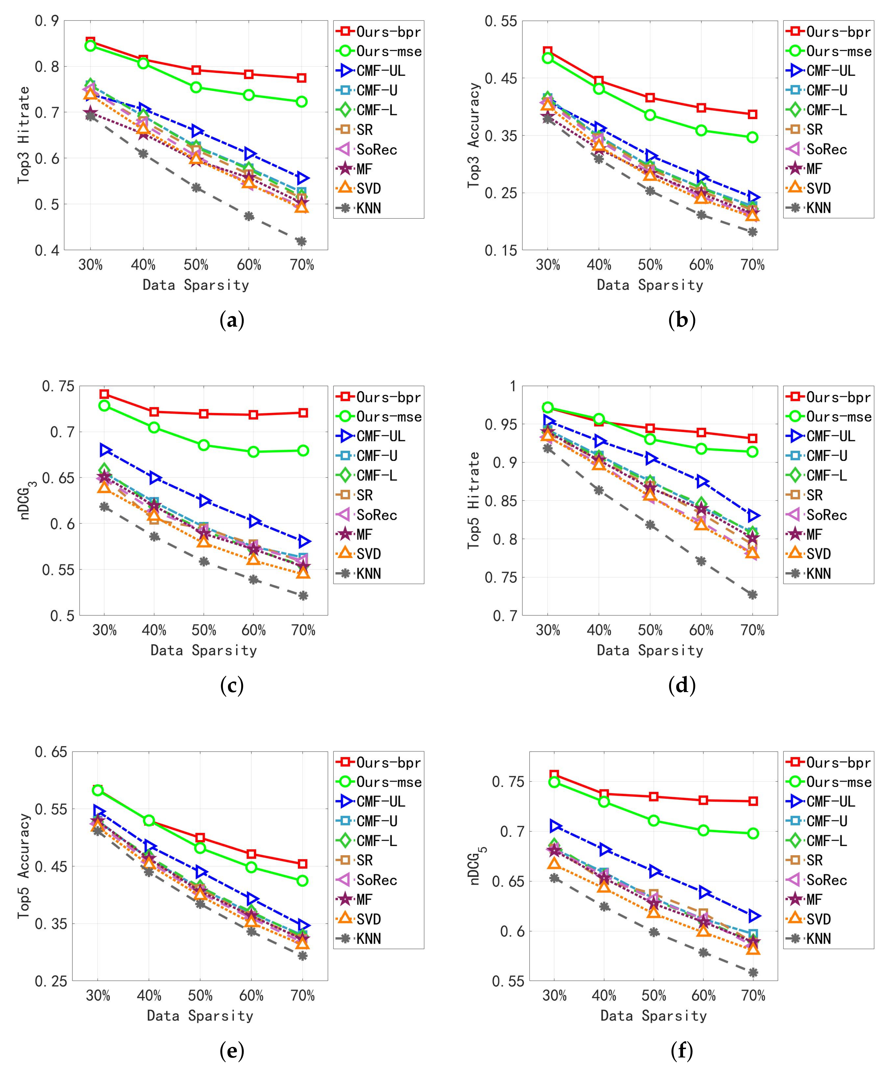
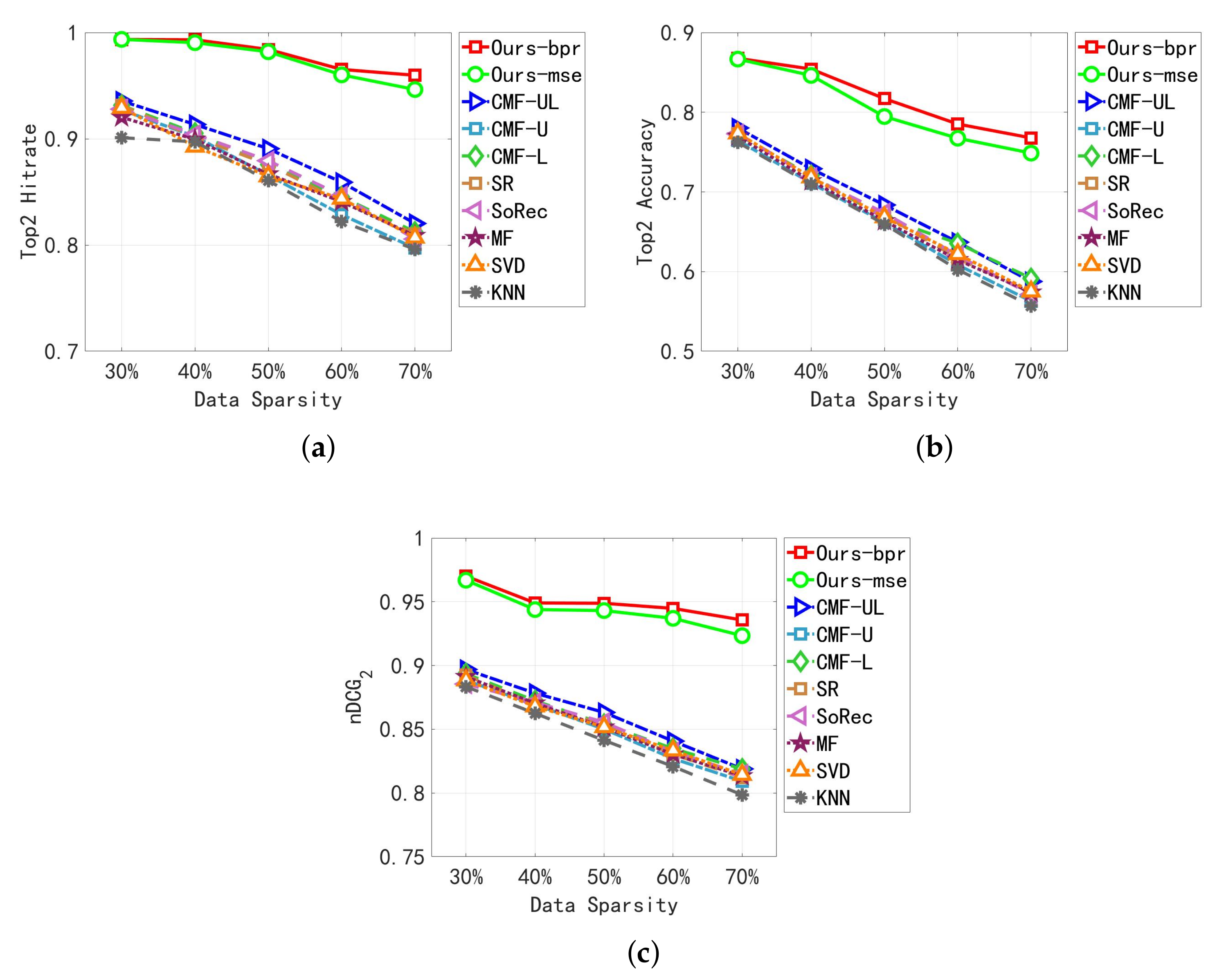
5.2.1. Results Analyses

It can be seen from the Table 2, Figure 4 and Figure 5 that compared with other methods, our model provides the best recommendation results. In Table 2, the best results are highlighted with Bold style.
Take the data sparsity level of 50% as an example shown in Table 2. Our model achieves the best performance with BPRLoss. It can be seen from Table 2 that it achieves 13.20%, 10.1%, and 9.44% higher than the best baseline model, CMF-UL, in T o p 3 H i t r a t e , T o p 3 A c c u r a c y , and n D C G 3 , respectively, in the Telecom dataset. In the TalkingData dataset, our model also achieves 9.34%, 13.35%, and 8.56% than CMF-UL in T o p 2 H i t r a t e , T o p 2 A c c u r a c y , and n D C G 2 , respectively. Comparing two different loss functions, our model achieves higher score with BPRLoss because it takes users’ preferences into consideration and strengthens the ranking comparison. Obviously, our model significantly outperforms cooperative tensor factorization and other machine learning methods in location recommendations. It is because that our model can aggregate high-order interactions of user–user, user–location, and location–location with app usage patterns, which lead to more precise representations, while CMF-UL cannot. It also proves our hypothesis H 3 that user interests and location characters can be associated by app records, so that we can extract their high-order interactions. Moreover, it can be seen that our model and CMF-UL outperforms other baselines with using app records, which can verify our hypotheses H 1 and H 2 that app usage is associated with user interests and location characteristics.
Furthermore, our representation model shows the best recommendation performance at all sparsity levels. Especially it can provide larger improvements under high sparsity. We compare the results under 70% and 30% data sparsity. In the Telecom dataset, when the data sparsity is 30%, the T o p 3 H i t r a t e , T o p 3 A c c u r a c y , and n D C G 3 of our model are 11.42%, 8.19%, and 6.07% higher than the best baseline model, respectively. While data sparsity is 70%, T o p 3 H i t r a t e , T o p 3 A c c u r a c y , and n D C G 3 of our model achieve at least 21.76%, 14.47%, and 14.00% higher than the best baseline model, respectively. On the TalkingData dataset, when the data sparsity is 30%, T o p 2 H i t r a t e , T o p 2 A c c u r a c y , and n D C G 2 of our model are 5.8%, 8.74%, and 7.32% higher than other models, respectively. However, our model achieves 13.95%, 18.02%, and 11.68% improvements in T o p 2 H i t r a t e , T o p 2 A c c u r a c y , and n D C G 2 , respectively, under 70% data sparsity. These results show that our model can effectively deal with the data sparsity problem.

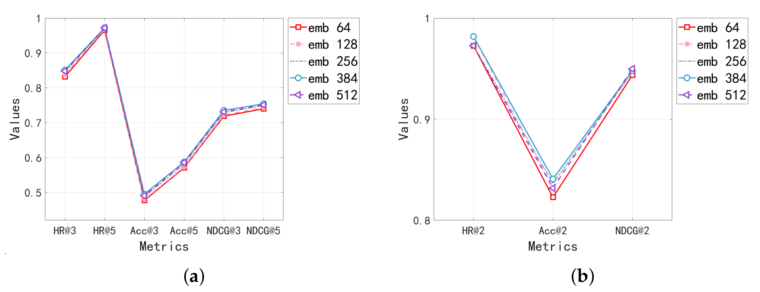
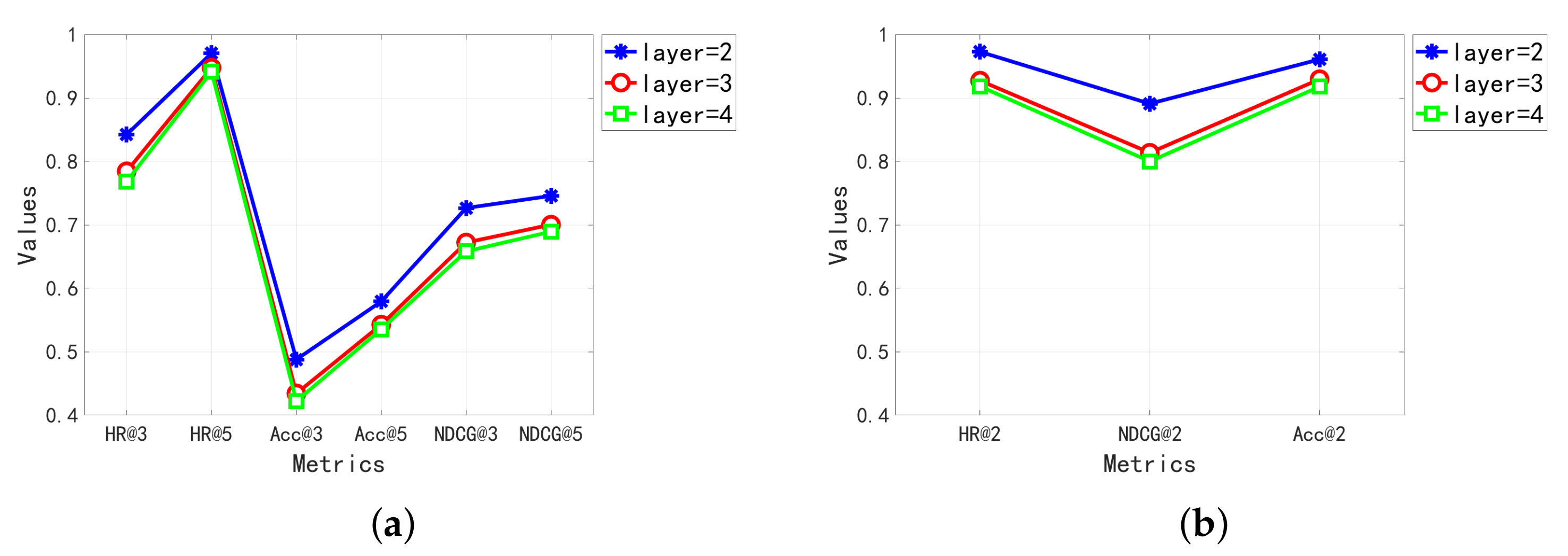
5.2.2. Parameter Study

We study the model performances with different values of two important hyperparameters: the embedding dimension and the layers of our model under 30% data sparsity. For each experiment, only the target hyperparameter is changed to observe the optimal one under different evaluation metrics. As shown in Figure 6, the best embedding dimension is 384 on both datasets. The best number of graph convolutional layers is two, as shown in Figure 7. The deeper layer may cause the over-smoothing problem in GCN [54], which leads to worse results.

6. Conclusions

In conclusion, we propose a graph-based representation model in this paper that greatly improves location recommendation results with app usage records and solves the data sparsity problem. Firstly, we analyze the data sparsity problem in personalized location recommendations and discuss the feasibility of app usage records. Then, the representation model with attributed bipartite graph is introduced in detail. The experiment results show that compared with the state-of-art models, our proposed model has the best recommendation performance under different data sparsity levels. Especially, when facing a severe sparsity problem, the performance of our model has greater improvements due to the aggregations of user–app–location interactions. Additionally, it also further confirms the strong correlation between app data usage, user interests and location characteristics. This is a successful attempt to discover deep representations of users and locations via attributed graph-based network.
To sum up, the main contributions of our paper are summarized as follows:
1.
To the best of our knowledge, it is the first to solve the data sparsity problem in location recommendations by aggregating user–app–location associations, which can also inspire the research works about users’ app usage behavior. We innovatively introduce app usage records as complementary information, in which both users’ habits and location features are revealed. This method effectively alleviates the data sparsity problem and greatly improves the recommendation performances.
2.
A graph-based representation model is proposed to learn both users’ and locations’ latent representations from an attributed bipartite graph. Our model explicitly uses associations of user-app-location, and captures various high-order features due to the information propagation and aggregation in graph structure. Therefore, it can significantly improve location recommendations, even under the circumstances of severe data sparsity.
3.
Adequate experiments are conducted on two real-life datasets to show the superior and stable performance of our proposed model. Our model achieves the best performance compared with the state-of-art methods. It also works well under severe data sparsity, which has a higher increase in recommending performances when facing higher sparsity. For example, in Telecom dataset, when the data sparsity is 30%, T o p 3 H i t r a t e , T o p 3 A c c u r a c y , and n D C G 3 of our model are 11.42%, 8.19%, and 6.07% higher than the best baseline model, respectively. While data sparsity is 70%, T o p 3 H i t r a t e , T o p 3 A c c u r a c y , and n D C G 3 of our model achieve performances at least 21.76%, 14.47%, and 14.00% higher than the best baseline model, respectively.
In practical application, our proposed model can be employed to improve user experiences, user profile extraction and user app behaviors extraction, etc. However, there are still limitations in this paper, such as not considering long-term factors (i.e., user preferences changing) and short-term time affects (i.e., specific time points in a day). In future work, these temporal features will be taken into consideration and multi-head attention structure can be applied to discover more associations among users, locations and apps, which can improve recommendation results.

Author Contributions

Conceptualization, X.C. and J.C.; methodology, X.C. and J.C.; software, J.C; validation, X.C., J.C. and X.L.; formal analysis, X.C. and J.C.; investigation, W.M.; writing original draft preparation, J.C.; writing, review and editing, X.C., J.C. and X.L.; visualization, J.C. and W.M.; supervision, X.C. and W.M.; project administration, X.C. and X.L.; funding acquisition, X.C. and X.L. All authors have read and agreed to the published version of the manuscript.

Funding

This work was supported by the National Key Research and Development Program of China (No. 2019YFE0196400), Guangdong R&D Project in Key Areas under Grant (No. 2019B010158001), and the Open Research Fund Program of Key Laboratory of Industrial Internet and Big Data, China National Light Industry, Beijing Technology and Business University (No. IIBD-2020-KF04).

Institutional Review Board Statement

Not applicable.

Informed Consent Statement

Not applicable.

Data Availability Statement

The data used in this research can be found in the references we provide in the article.

Conflicts of Interest

The authors declare no conflict of interest.

Abbreviations

The following abbreviations are used in this manuscript:
RNNRecurrent Neural Network
GCNGraph Convolutional Network
CNNConvolutional Neural Network
LSTMLong Short-Term Memory
POIPoint of Interest
GRUGated Recurrent Unit
SVD-MFNSingular Value Decomposition with Multi-Factor Neighborhood
KNNK-Nearest Neighbor

References

  1. Werneck, H.; Silva, N.; Viana, M.C.; Mourão, F.; Pereira, A.C.M.; Rocha, L. A Survey on Point-of-Interest Recommendation in Location-Based Social Networks. In Proceedings of the Brazilian Symposium on Multimedia and the Web, São Luís, Brazil, 30 November–4 December 2020; Association for Computing Machinery: New York, NY, USA, 2020; pp. 185–192. [Google Scholar] [CrossRef]
  2. Zhu, D.H.; Chang, Y.P.; Luo, J.J.; Li, X. Understanding the adoption of location-based recommendation agents among active users of social networking sites. Inf. Process. Manag. 2014, 50, 675–682. [Google Scholar] [CrossRef]
  3. Wu, C.; Kao, S.C.; Wu, C.C.; Huang, S. Location-aware service applied to mobile short message advertising: Design, development, and evaluation. Inf. Process. Manag. 2015, 51, 625–642. [Google Scholar] [CrossRef]
  4. Bao, J.; Zheng, Y.; Wilkie, D.; Mokbel, M.F. Recommendations in location-based social networks: A survey. GeoInformatica 2015, 19, 525–565. [Google Scholar] [CrossRef]
  5. Lian, D.; Zhao, C.; Xie, X.; Sun, G.; Chen, E.; Rui, Y. GeoMF: Joint geographical modeling and matrix factorization for point-of-interest recommendation. In Proceedings of the The 20th ACM SIGKDD International Conference on Knowledge Discovery and Data Mining, KDD’14, New York, NY, USA, 24–27 August 2014; ACM: New York, NY, USA, 2014; pp. 831–840. [Google Scholar] [CrossRef]
  6. Lian, D.; Zheng, K.; Ge, Y.; Cao, L.; Chen, E.; Xie, X. GeoMF++: Scalable Location Recommendation via Joint Geographical Modeling and Matrix Factorization. ACM Trans. Inf. Syst. 2018, 36, 33:1–33:29. [Google Scholar] [CrossRef]
  7. Zhong, C.; Zhu, J.; Xi, H. PS-LSTM: Popularity Analysis And Social Network For Point-Of-Interest Recommendation In Previously Unvisited Locations. In Proceedings of the CNIOT 2021: 2nd International Conference on Computing, Networks and Internet of Things, Beijing, China, 20–22 May 2021; ACM: New York, NY, USA, 2021; pp. 28:1–28:6. [Google Scholar] [CrossRef]
  8. Luo, Y.; Liu, Q.; Liu, Z. STAN: Spatio-Temporal Attention Network for Next Location Recommendation. In Proceedings of the WWW’21: The Web Conference 2021, Ljubljana, Slovenia, 19–23 April 2021; ACM/IW3C2: New York, NY, USA, 2021; pp. 2177–2185. [Google Scholar] [CrossRef]
  9. Ameen, T.; Chen, L.; Xu, Z.; Lyu, D.; Shi, H. A Convolutional Neural Network and Matrix Factorization-Based Travel Location Recommendation Method Using Community-Contributed Geotagged Photos. ISPRS Int. J. Geo Inf. 2020, 9, 464. [Google Scholar] [CrossRef]
  10. Xu, H.; Wang, J.; Wei, J. Recommending irregular regions using graph attentive networks. Ad Hoc Networks 2021, 113, 102383. [Google Scholar] [CrossRef]
  11. Guo, Z.; Wang, H. A Deep Graph Neural Network-Based Mechanism for Social Recommendations. IEEE Trans. Ind. Inform. 2021, 17, 2776–2783. [Google Scholar] [CrossRef]
  12. Liu, X.; Song, R.; Wang, Y.; Xu, H. A Multi-Granular Aggregation-Enhanced Knowledge Graph Representation for Recommendation. Information 2022, 13, 229. [Google Scholar] [CrossRef]
  13. Hu, B.; Ye, Y.; Zhong, Y.; Pan, J.; Hu, M. TransMKR: Translation-based knowledge graph enhanced multi-task point-of-interest recommendation. Neurocomputing 2022, 474, 107–114. [Google Scholar] [CrossRef]
  14. Cai, X.; Xie, L.; Tian, R.; Cui, Z. Explicable recommendation based on knowledge graph. Expert Syst. Appl. 2022, 200, 117035. [Google Scholar] [CrossRef]
  15. Singh, M. Scalability and sparsity issues in recommender datasets: A survey. Knowl. Inf. Syst. 2020, 62, 1–43. [Google Scholar] [CrossRef]
  16. Zheng, L.; Li, C.; Lu, C.; Zhang, J.; Yu, P.S. Deep Distribution Network: Addressing the Data Sparsity Issue for Top-N Recommendation. In Proceedings of the 42nd International ACM SIGIR Conference on Research and Development in Information Retrieval, Paris, France, 21–25 July 2019; ACM: Paris, France, 2019; pp. 1081–1084. [Google Scholar]
  17. Liu, Y.; Pham, T.; Cong, G.; Yuan, Q. An Experimental Evaluation of Point-of-interest Recommendation in Location-based Social Networks. Proc. VLDB Endow. 2017, 10, 1010–1021. [Google Scholar] [CrossRef]
  18. Long, X.; Joshi, J. A HITS-based POI recommendation algorithm for location-based social networks. In Proceedings of the Advances in Social Networks Analysis and Mining, Niagara, ON, Canada, 25–28 August 2013; ACM: Niagara, ON, Canada, 2013; pp. 642–647. [Google Scholar]
  19. Gao, H.; Tang, J.; Liu, H. Addressing the cold-start problem in location recommendation using geo-social correlations. Data Min. Knowl. Discov. 2015, 29, 299–323. [Google Scholar] [CrossRef] [Green Version]
  20. Yu, F.; Cui, L.; Guo, W.; Lu, X.; Li, Q.; Lu, H. A Category-Aware Deep Model for Successive POI Recommendation on Sparse Check-in Data. In Proceedings of the Web Conference 2020, Taipei, Taiwan, 20–24 April 2020; ACM/IW3C2: Taipei, Taiwan, 2020; pp. 1264–1274. [Google Scholar]
  21. Guo, H.; Li, X.; He, M.; Zhao, X.; Liu, G.; Xu, G. CoSoLoRec: Joint Factor Model with Content, Social, Location for Heterogeneous Point-of-Interest Recommendation. In Proceedings of the Knowledge Science, Engineering and Management—9th International Conference, KSEM 2016, Passau, Germany, 5–7 October 2016; Lecture Notes in Computer Science. Volume 9983, pp. 613–627. [Google Scholar] [CrossRef] [Green Version]
  22. Ma, Y.; Mao, J.; Ba, Z.; Li, G. Location recommendation by combining geographical, categorical, and social preferences with location popularity. Inf. Process. Manag. 2020, 57, 102251. [Google Scholar] [CrossRef]
  23. Tu, Z.; Fan, Y.; Li, Y.; Chen, X.; Su, L.; Jin, D. From Fingerprint to Footprint: Cold-start Location Recommendation by Learning User Interest from App Data. Proc. ACM Interact. Mob. Wearable Ubiquitous Technol. 2019, 3, 26:1–26:22. [Google Scholar] [CrossRef]
  24. Su, Y.; Li, X.; Zha, D.; Tang, W.; Jiang, Y.; Xiang, J.; Gao, N. HRec: Heterogeneous Graph Embedding-Based Personalized Point-of-Interest Recommendation. In Proceedings of the ICONIP, Bangkok, Thailand, 8–12 December 2019; Lecture Notes in Computer Science. Volume 11955, pp. 37–49. [Google Scholar]
  25. Hu, X.; Xu, J.; Wang, W.; Li, Z.; Liu, A. A graph embedding based model for fine-grained POI recommendation. Neurocomputing 2021, 428, 376–384. [Google Scholar] [CrossRef]
  26. Huang, Z.; Chen, H.; Zeng, D.D. Applying associative retrieval techniques to alleviate the sparsity problem in collaborative filtering. ACM Trans. Inf. Syst. 2004, 22, 116–142. [Google Scholar] [CrossRef] [Green Version]
  27. Xie, H.; Fan, Q.; Xiao, Q. A Social Collaborative Filtering Method to Alleviate Data Sparsity Based on Graph Convolutional Networks. IEICE Trans. Inf. Syst. 2020, 103-D, 2611–2619. [Google Scholar] [CrossRef]
  28. Natarajan, N.; Shin, D.; Dhillon, I.S. Which app will you use next? Collaborative filtering with interactional context. In Proceedings of the the 7th ACM Conference on Recommender Systems, Hong Kong, China, 12–16 October 2013; ACM: Hong Kong, China, 2013; pp. 201–208. [Google Scholar]
  29. Zou, X.; Zhang, W.; Li, S.; Pan, G. Prophet: What app you wish to use next. In Proceedings of the The 2013 ACM International Joint Conference on Pervasive and Ubiquitous Computing, Zurich, Switzerland, 8–12 September 2013; ACM: Zurich, Switzerland, 2013; pp. 167–170. [Google Scholar]
  30. Baeza-Yates, R.; Jiang, D.; Silvestri, F.; Harrison, B. Predicting The Next App That You Are Going To Use. In Proceedings of the Eighth ACM International Conference on Web Search and Data Mining, Shanghai, China, 2–6 February 2015; ACM: Shanghai, China, 2015; pp. 285–294. [Google Scholar]
  31. Xia, B.; Ni, Z.; Li, T.; Li, Q.; Zhou, Q. VRer: Context-Based Venue Recommendation using embedded space ranking SVM in location-based social network. Expert Syst. Appl. 2017, 83, 18–29. [Google Scholar] [CrossRef]
  32. Lyu, D.; Chen, L.; Xu, Z.; Yu, S. Weighted multi-information constrained matrix factorization for personalized travel location recommendation based on geo-tagged photos. Appl. Intell. 2020, 50, 924–938. [Google Scholar] [CrossRef]
  33. Yin, Y.; Chen, L.; Xu, Y.; Wan, J. Location-Aware Service Recommendation With Enhanced Probabilistic Matrix Factorization. IEEE Access 2018, 6, 62815–62825. [Google Scholar] [CrossRef]
  34. Yang, D.; Zhang, D.; Yu, Z.; Wang, Z. A sentiment-enhanced personalized location recommendation system. In Proceedings of the 24th ACM Conference on Hypertext and Social Media (Part of ECRC), Paris, France, 1–3 May 2013; ACM: Paris, France, 2013; pp. 119–128. [Google Scholar]
  35. Qi, M.; Ma, W.; Shan, R. Design and Implementation of Tourist Location Recommendation System Based on Recurrent Neural Network. Electron. Technol. Softw. Eng. 2020, 1, 184–185. [Google Scholar]
  36. Zhao, P.; Zhu, H.; Liu, Y.; Xu, J.; Zhou, X. Where to Go Next: A Spatio-Temporal Gated Network for Next POI Recommendation. Proc. AAAI Conf. Artif. Intell. 2019, 33, 5877–5884. [Google Scholar] [CrossRef]
  37. Zhou, F.; Yin, R.; Zhang, K.; Trajcevski, G.; Zhong, T.; Wu, J. Adversarial Point-of-Interest Recommendation. In Proceedings of the The World Wide Web Conference, San Francisco, CA, USA, 13–17 May 2019; ACM: San Francisco, CA, USA, 2019; pp. 3462–34618. [Google Scholar]
  38. Kipf, T.N.; Welling, M. Semi-Supervised Classification with Graph Convolutional Networks. In Proceedings of the The 5th International Conference on Learning Representations, Toulon, France, 24–26 April 2017; OpenReview.net: Toulon, France, 2017. [Google Scholar]
  39. Wang, X.; He, X.; Wang, M.; Feng, F.; Chua, T. Neural Graph Collaborative Filtering. In Proceedings of the 42nd International ACM SIGIR Conference on Research and Development in Information Retrieval, SIGIR 2019, Paris, France, 21–25 July 2019; Piwowarski, B., Chevalier, M., Gaussier, É., Maarek, Y., Nie, J., Scholer, F., Eds.; ACM: New York, NY, USA, 2019; pp. 165–174. [Google Scholar] [CrossRef] [Green Version]
  40. Canturk, D.; Karagoz, P. SgWalk: Location Recommendation by User Subgraph-Based Graph Embedding. IEEE Access 2021, 9, 134858–134873. [Google Scholar] [CrossRef]
  41. Xu, S.; Cao, J.; Legg, P.; Liu, B.; Li, S. Venue2Vec: An Efficient Embedding Model for Fine-Grained User Location Prediction in Geo-Social Networks. IEEE Syst. J. 2020, 14, 1740–1751. [Google Scholar] [CrossRef] [Green Version]
  42. Zhong, T.; Zhang, S.; Zhou, F.; Zhang, K.; Trajcevski, G.; Wu, J. Hybrid graph convolutional networks with multi-head attention for location recommendation. World Wide Web 2020, 23, 3125–3151. [Google Scholar] [CrossRef]
  43. Huang, D.; Chen, G.; Haibing Li et, a. Spark personalized location recommendation system. J. Liaoning Tech. Univ. Nat. Sci. Ed. 2020, 39, 533–540. [Google Scholar]
  44. Xia, T.; Li, Y.; Feng, J.; Jin, D.; Zhang, Q.; Luo, H.; Liao, Q. DeepApp: Predicting Personalized Smartphone App Usage via Context-Aware Multi-Task Learning. Trans. Interact. Intell. Syst. 2020, 11, 64:1–64:12. [Google Scholar] [CrossRef]
  45. Lee, Y.; Park, I.; Cho, S.; Choi, J. Smartphone user segmentation based on app usage sequence with neural networks. Telemat. Inform. 2018, 35, 329–339. [Google Scholar] [CrossRef]
  46. Xia, T.; Li, Y. Revealing Urban Dynamics by Learning Online and Offline Behaviours Together. Proc. ACM Interact. Mob. Wearable Ubiquitous Technol. 2019, 3, 30:1–30:25. [Google Scholar] [CrossRef]
  47. Yu, D.; Li, Y.; Xu, F.; Zhang, P.; Kostakos, V. Smartphone App Usage Prediction Using Points of Interest. Proc. ACM Interact. Mob. Wearable Ubiquitous Technol. 2017, 1, 174:1–174:21. [Google Scholar] [CrossRef] [Green Version]
  48. 2018, K. TalkingData Mobile User Demographics. Available online: https://www.kaggle.com/c/talkingdata-mobile-user-demographics (accessed on 11 October 2018).
  49. He, X.; Deng, K.; Wang, X.; Li, Y.; Zhang, Y.; Wang, M. LightGCN: Simplifying and Powering Graph Convolution Network for Recommendation. In Proceedings of the 43rd International ACM SIGIR Conference on Research and Development in Information Retrieval, Virtual, 11–15 July 2020; ACM: New York, NY, USA, 2020; pp. 639–648. [Google Scholar]
  50. Rendle, S.; Freudenthaler, C.; Gantner, Z.; Schmidt-Thieme, L. BPR: Bayesian Personalized Ranking from Implicit Feedback. In Proceedings of the Twenty-Fifth Conference on Uncertainty in Artificial Intelligence, Montreal, QC, Canada, 18–21 June 2009; pp. 452–461. [Google Scholar]
  51. Rong, D.; Yu, Z.; Tao, M.; Wang, Z.; Guo, B. Predicting activity attendance in event-based social networks: Content, context and social influence. In Proceedings of the ACM International Joint Conference on Pervasive and Ubiquitous Computing, Seattle, WA, USA, 13–17 September 2014; ACM: Seattle, WA, USA, 2014; pp. 425–434. [Google Scholar]
  52. Hao, M.; Yang, H.; Lyu, M.R.; King, I. SoRec: Social recommendation using probabilistic matrix factorization. In Proceedings of the 17th ACM Conference on Information and Knowledge Management, Napa Valley, CA, USA, 26–30 October 2008; ACM: Napa Valley, CA, USA, 2008; pp. 931–940. [Google Scholar]
  53. Ma, H.; Zhou, D.; Liu, C.; Lyu, M.R.; King, I. Recommender systems with social regularization. In Proceedings of the Forth International Conference on Web Search and Web Data Mining, Hong Kong, China, 21–25 February 2011; pp. 287–296. [Google Scholar]
  54. Elinas, P.; Bonilla, E.V. Addressing Over-Smoothing in Graph Neural Networks via Deep Supervision. arXiv 2022, arXiv:2202.12508. [Google Scholar]
Figure 1. Illustration of statistics of Telecom dataset. (a) Number of locations per user. (b) App/app category differences. (c) App usage in different locations. (d) Location differences.
Applsci 12 06882 g001
Figure 2. Our Proposed Personalized Location Recommending Framework based on app data.
Applsci 12 06882 g002
Figure 3. The “User-Location” Bipartite Graph G and the Information Propagation in Graph Convolution. (a) The Schematic of “User-Location” Bipartite Graph. (b) The Information Propagation of Graph Convolution.
Applsci 12 06882 g003
Figure 4. Comparisons of the Recommendation Performances on Telecom Dataset under Different Sparsity Levels. (a) T o p 3 H i t r a t e . (b) T o p 3 A c c u r a c y . (c) n D C G 3 . (d) T o p 5 H i t r a t e . (e) T o p 5 A c c u r a c y . (f) n D C G 5 .
Applsci 12 06882 g004
Figure 5. Comparisons of the Recommendation Performances on TalkingData Dataset under Different Sparsity Levels. (a) T o p 2 H i t r a t e . (b) T o p 2 A c c u r a c y . (c) n D C G 2 .
Applsci 12 06882 g005
Figure 6. Performances of Different Embedding Dimensions on Two Datasets. (a) T e l e c o m D a t a s e t . (b) T a l k i n g D a t a s e t .
Applsci 12 06882 g006
Figure 7. Performances of Different Layers on Two Datasets. (a) T e l e c o m D a t a s e t . (b) T a l k i n g D a t a s e t .
Applsci 12 06882 g007
Table 1. Datasets and Statistics Information.
Telecom DatasetTalkingData
Data SourcesCellular networkMobile application
CityShanghai, ChinaGuangzhou, China
Time Duration20–26 April 20161–7 May 2016
Records40,470,865180,106
Users10,000256
Locations11,584439
Apps1327689
Table 2. Recommendation Results Under 50% Data Sparsity.
DatasetTelecom DatasetTalkingData
HR@3ACC@3nDCG@3HR@5ACC@5nDCG@5HR@2ACC@2nDCG@2
KNN0.53590.25340.55860.81850.38410.59900.86060.65960.8413
SVD0.59680.27840.57880.85570.39850.61740.86480.66830.8517
MF0.59680.28310.58900.86640.40620.62740.86680.66360.8516
SoRec0.60450.28490.59190.85480.40350.63180.87940.67380.8555
SR0.61840.29110.59490.86970.41030.63720.87590.67080.8538
CMF-L0.62330.29450.59260.87360.41350.63170.87560.66750.8540
CMF-U0.62580.29610.59650.87540.41140.63270.86570.66170.8501
CMF-UL0.65960.31460.62500.90530.44030.66000.89070.68360.8632
Ours-mse0.75430.38550.68540.93030.48170.71070.98190.79460.9431
Ours-bpr0.79160.41560.71940.94460.49970.73470.98410.81710.9488
Publisher’s Note: MDPI stays neutral with regard to jurisdictional claims in published maps and institutional affiliations.

