Normality in the Distribution of Revealed Comparative Advantage Index for International Trade and Economic Complexity

Abstract

The Revealed Comparative Advantage (RCA) index is an important metric for evaluating competitiveness of a country in exporting certain commodity. While it is desirable to have a normally distributed RCA index, the opposite is often found in empirical studies, and efforts for developing alternative indices of the RCA index have not been very successful. This motivates us to ask a more fundamental question: what is the significance of a normally distributed RCA index? To answer this question, we have defined a quantity called the Deviation from Gaussianity (DfG) based on the KS test, which quantifies the deviation of the distribution of a country’s RCA index from normality. By systematically analyzing the distribution characteristics of RCA index for each country from 1991 to 2019, we find that DfG is strongly negatively correlated with the logarithm of GDP and the Economic Complexity Index (ECI). In particular, correlation between DfG and GDP is stronger than that between ECI and GDP since 2008. These results suggest that DfG may serve as a new excellent index to quantify the economic complexity and economic performance of a country.

1. Introduction

The revealed comparative advantage (RCA) index, also called Balassa index as it was first proposed by Balassa in 1965 [1], is an important metric for quantifying the relative strength of a country in producing a product vis-à-vis its trading partners. While it has been widely used in empirical studies, the RCA index has also been further studied theoretically. Those works mainly focus on the statistical features of the RCA index, and can be roughly classified into two groups. One group is somewhat traditional, with emphasis on clarifying the statistical characteristics of the RCA index across sectors or countries. In many applications, it is desirable to have a normally distributed RCA index, so that it can reliably measure a country’s revealed comparative advantage [2]. However, in the majority of empirical studies, a non-Gaussian distribution of the RCA index has been observed. The non-Gaussianity has made the RCA index to suffer from many disturbing properties such as unstable distribution and poor ordinal ranking property [3], the unstable mean [4,5], asymmetric distributional shape [2], and skewness and variable upper bound [6,7]. These features of the RCA index have made its interpretation difficult [3,4,8,9,10], and thus have motivated a lot of researchers to develop alternative indices of the RCA index so that the new indices can be more normally distributed [3,4,5,11,12,13,14,15]. These efforts are not very successful, however. To understand why the RCA index and its alternatives may not follow Gaussian distributions, Liu and Gao systematically analyzed the distribution characteristics of the RCA index cross sectors and countries [16]. They find that the RCA index in the majority of the situations cannot be normally distributed, since it is the ratio of two distributions, one following an exponentially truncated Zipf–Mandelbrot’s law, the other being a permutation of the truncated Zipf–Mandelbrot’s law [16]. Only occasionally can a normally distributed RCA index be observed—it may emerge with about 1% chance. The significance of a normally distributed RCA index has not yet been explained, however.

The other group of the work on the theoretical aspects of the RCA index mainly employs matrix and complex network theory by constructing the country–product bipartite network, where countries are connected to the products they export. The bipartite network is an 0–1 adjacency matrix constructed according to the value of the RCA index (the element is 1 if the corresponding RCA $\ge 1$ and 0 otherwise). By developing the Method of Reflections to interpret an export bipartite network, Hidalgo and Hausmann proposed the Economic Complexity Index (ECI) and Product Complexity Index (PCI) [17,18]. Hidalgo and Hausmann’s approach has been proven to be equivalent to a spectral clustering algorithm that partitions a similarity graph into two parts [19]. Although, the ECI may offer a good description of global macroeconomic relations, technological trends, and growth dynamics [20], and could be used to measure the gap in the economic development between countries [21], the approach suffers from a number of conceptual and practical problems [22,23,24,25,26]. To overcome these problems, the Fitness Index (FI) and some other variants of the ECI have been developed [22,23,24,27,28]. The ECI and its variants have been widely used to study the impact of economic structures on economic development [18,20,29,30,31,32,33,34,35,36,37,38,39,40,41,42]. Fundamentally speaking, however, the FI and the other new variants of the ECI are not very different from the ECI, since the ECI and FI (or $log\mathrm{FI}$) are strongly positively correlated [37,38,39,40,41], and both metrics have almost the same skill in predicting economic growth [42]. This raises an important question as to which of the neglected aspects of the RCA index by the network based approach should be reinstated so that characterization of economic complexity can be fundamentally improved.

In this article, we attempt to answer both the above questions: why a normally distributed RCA index is important and how to better quantify economic complexity. In doing so, we will find a bridge connecting the two groups, one more traditional, the other based on the network approach. Concretely, we will define a quantify called the Deviation from Gaussianity (DfG) based on the KS test, which measures the deviation of the distribution of a country’s RCA index from normality. Then, we will systematically analyze the distribution characteristics of RCA index for each country from 1991 to 2019, and examine the relationship between the DfG and economic development and economic complexity.

The remainder of the paper is organized as follows: Section 2 describes Materials and methods, Section 3 presents the main results, and Section 4 contains conclusion and discussion.

2. Materials and Methods

2.1. Materials

In this work, we analyze international commodity trade data with products disaggregated according to the COMTRADE Harmonized System at the four-digital level (abbreviated as HS4). The data covered 29 years from 1991 to 2019, and were downloaded from UNComtrade database (International Trade Statistics Database: https://comtrade.un.org/ accessed on 5 August 2021 ).

2.2. Methods

2.2.1. RCA Index

The RCA index is defined as

$${\mathrm{RCA}}_{\left(ix\right)}^k=\frac{X_{\left(i\right)}^k/X_{\left(i\right)}}{X_{\left(w\right)}^k/X_{\left(w\right)}}=\frac{p_{\left(ix\right)}^k}{p_{\left(wx\right)}^k},$$

(1)

where X (or x) denotes export, i denotes country, while w denotes world, k denotes product. For example, $X_{\left(i\right)}^k$ represents country i’s export of product k, $X_{\left(i\right)}$ denotes country i’s total export, and $X_{\left(i\right)}^k/X_{\left(i\right)}$ is the export share of country i in product k. Being a probability, it can also be expressed as $p_{\left(ix\right)}^k$, and ${\sum }_{k=1}^{N_c}{p}_{\left(ix\right)}^k=1$, where $N_c$ represents the number of products in a country.

2.2.2. Economic Complexity Index

The Economic Complexity Index (ECI) was developed by Hidalgo and Hausmann in 2009 [18]. The algorithm for computing it is as follows. Consider a country-product bipartite network represented by a matrix with elements $M_{cp}$ defined as 1 or 0, depending on whether the corresponding RCA $\ge 1$ or RCA $<1$. Summing up rows and columns of the matrix, one obtains $k_{c,0}={\sum }_p{M}_{cp}$, $k_{p,0}={\sum }_c{M}_{cp}$, which represent, respectively, the observed the number of products exported by some country, and the number of countries exporting some product. The ECI is obtained by an iteration algorithm,

$$k_{c,N}=\frac{1}{k_{c,0}}\sum _p{M}_{cp}{k}_{p,N-1},$$

(2)

$$k_{p,N}=\frac{1}{k_{p,0}}\sum _p{M}_{cp}{k}_{c,N-1},$$

(3)

where $N\ge 2$ is the number of iterations. Collecting $k_{c,N},c=1,\cdots ,C_n$, where $C_n$ is the total number of countries with data, we then obtain ECI as

$${\mathrm{ECI}}_{c^{*}}=\frac{k_{c^{*},N}-\mathrm{mean}\left\{k_{c,N}\right\}}{\mathrm{stdev}\left\{k_{c,N}\right\}},$$

(4)

where $c^{*}$ denotes a country of interest, and mean and stdev are performed over all the countries with data. It is thought that the larger the ECI, the higher the economic complexity.

2.2.3. Deviation from Gaussianity Based on KS Test

The KS test (Kolmogorov–Smirnov test or K-S test) is one of the most useful and general nonparametric methods. The one-sample KS test can be used to compare a sample with a reference probability distribution. In this paper, we define the Deviation from Gaussianity (DfG) based on one-sample KS test. The algorithm is as follows:

$$F_n\left(x\right)=\frac{1}{n}\sum _{n=1}^N{I}_{[-\infty ,x]}\left(X_i\right),$$

(5)

where $I_{[-\infty ,x]}\left(X_i\right)$ is the indicator function, which is equal to 1 if $X_i<x$ and 0 otherwise. The Kolmogorov–Smirnov statistic for a given cumulative distribution function $F\left(x\right)$ is

$$D_n={sup}_x|F_n\left(x\right)-F\left(x\right)|,$$

(6)

where $su{p}_x$ is the supremum of the set of distances. We define the divergence of DfG in the distribution of RCA index as follows:

$$\mathrm{DfG}=D_n-CV,$$

(7)

where $CV$ is the critical value of KS test. A negative DfG indicates Gaussian distribution of RCA index, while a positive DfG indicates rejection of the Gaussian distribution—the more positive DfG, the larger the deviation from Gaussianity [16].

2.2.4. Pooled OLS and Panel VAR

In this article, we will also employ regression analysis to further explore the connections among DfG, ECI, and economic development. Considering that our data may be considered panel data, we will employ two regression models—pooled Ordinary Least Square (OLS) and panel Vector Autoregression (VAR) models. The general econometric model for panel data is as follows [43,44]:

$$Y_{it}={\alpha }_i+{\overrightarrow{\beta }}_i·{\overrightarrow{X}}_{it}+{\mu }_{it},$$

(8)

where, $i=1,2,\dots ,N$, $t=1,2,\dots ,T$, and N and T are the number of individual countries and total time (in year), respectively. $Y_{it}$ is the dependent variable, ${\overrightarrow{X}}_{it}$ is the independent variables (column vector), ${\alpha }_i$ and ${\overrightarrow{\beta }}_i$ are parameters (the latter a row vector with dimension matched to the column vector ${\overrightarrow{X}}_{it}$ so that the inner product is defined), and ${\mu }_{it}$ is the error term. As our purpose in this research is to find (and design) effective measures for quantifying economic complexity, we first assume that ${\alpha }_i$ and ${\overrightarrow{\beta }}_i$ are constant for all countries and time. This scenario is called the pooled OLS model, which is equivalent to the simple OLS model performed on panel data. The concrete equation used here is as follows:

$$ln{\mathrm{GDP}}_{it}=\alpha +{\beta }_1{\mathrm{DfG}}_{it}+{\beta }_2{\mathrm{ECI}}_{it}+{\mu }_{it},$$

(9)

We also use a panel-data VAR methodology. This technique combines the traditional VAR approach, which treats all the variables in the system as endogenous, with the panel-data approach, which allows for unobserved individual heterogeneity [45,46]. We employ a first-order panel VAR model as follows:

$$z_{i,t}={\Gamma }_0+{\Gamma }_1{z}_{i,t-1}+{\mu }_t,$$

(10)

where i represents the country in the panel-data, $z_{i,t}$ is a three-variable vector $(ln\mathrm{GDP},\mathrm{DfG},\mathrm{ECI})$, ${\Gamma }_1$ is a 3 × 3 matrix of coefficients, ${\Gamma }_0$ is a vector of individual effects. The stationarity of the three variables will be examined by using the LLC test [47] before we employ the PVAR model. Moreover, we can explore the statistical causality between the three variables based on the PVAR model.

3. Results

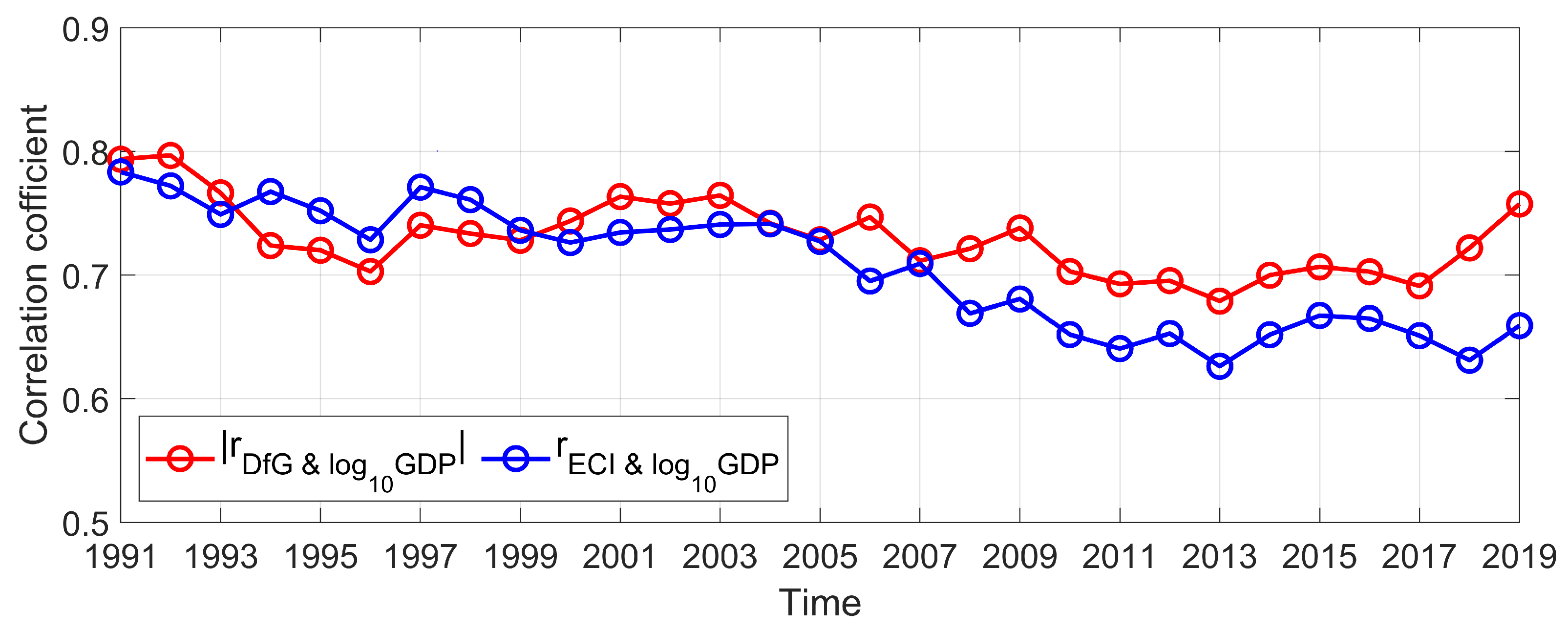
3.1. DfG and Economic Growth

There are two types of distributions for the RCA index. One is the distribution of the RCA index for all the sectors/products of an economy or a country. The other is the distribution of the RCA for all countries in the world given a sector/product. In this article, we focus on the former. Since the RCA index is the ratio of two probabilities, it is useful to first understand the distributions of the two probabilities. It turns out that both the numerator and the denominator defining the RCA index ($p_{\left(ix\right)}^k$ and $p_{\left(wx\right)}^k$) basically follow exponentially truncated Zipf–Mandelbrot’s law, given by:

$$p\left(k\right)\sim {(k+p)}^{-\alpha }{e}^{-\beta k^{{}^{\gamma }}},k>k^{*},$$

(11)

where p, $\alpha$, $\beta$, and $\gamma$ are parameters. The exponential truncation can be naturally expected due to finiteness of the data.

To better understand deviations from normality in the distribution of RCA index for different countries, we use Japan and Germany as two examples. Figure 1 shows the distribution features of the two parts of RCA index and the probability distribution function (PDF) of the RCA index for Japan and Germany under the HS4 scheme in 2018. Obviously, the $p_{\left(wx\right)}$ in Figure 1a,b follows exponentially truncated Zipf–Mandelbrot’s law. If the $p_{\left(ix\right)}$ in Figure 1a,b are also arranged in descending order, they will also follow exponentially truncated Zipf–Mandelbrot’s law (but possibly with different parameters). Interestingly, by comparing the layout of $p_{\left(ix\right)}$ (red diamonds) around $p_{\left(wx\right)}$ (blue circles) in Figure 1a,b, we can observe that the $p_{\left(ix\right)}$ of Germany is more concentrated around $p_{\left(wx\right)}$ than Japan’s. This highlights that Germany’s export share of most products relative to its total exports is closer to the world average level than Japan’s.

Next, we discuss how the differences between Figure 1a,b results in the differences in the distribution of the RCA index shown Figure 1c,d. Clearly, the PDFs for the RCA index of Germany and Japan are very different. Concretely, the PDF of Japan’s RCA index has more asymmetry, stronger skewness, and longer tail than that of Germany’s. This suggests that the PDF of Germany’s RCA index should be closer to a Gaussian distribution than Japan’s. To better quantify how the PDF of a country’s RCA index deviates from normality, we employ DfG we have defined earlier. The DfG for Germany and Japan is 0.088 and 0.266 in 2018, respectively. According to the nature of DfG—the more positive DfG, the larger the deviation from Gaussianity, one can conclude that the PDF of Germany’s RCA index is indeed closer to a normal distribution than that of Japan’s, just as one has anticipated from Figure 1.

It is interesting to examine the spatiotemporal evolution of the DfG of all the economies in the world. For this purpose, we have systematically computed DfG for all the economies in the world from 1991 to 2019. The spatial variations of the DfG in 1998, 2008 and 2018 are illustrated in Figure 2. We observe that the variations of DfG are characterized by spatiotemporal heterogeneity and regional spatial agglomeration.

First, let us focus on the spatiotemporal heterogeneity. From Figure 2a, we can observe: (1) only the DfG of USA and Germany was less than 0.1, followed by France and Italy, (2) only a few countries (such as China, South Korea, Japan, etc.) had DfG between 0.2 and 0.3, and (3) the DfG of most countries was greater than 0.3, especially in Africa, South America, Southern and Western Asia, and Eastern Europe. By 2008, which is shown in Figure 2b, the spatial variation of DfG had undergone some changes. Now Germany is the only economy with DfG $<0.1$, indicating that Germany is the only country with the PDF of its RCA index to be very close to a normal distribution. The decrease in China’s DfG was significant. In contrast, the DfG in some countries has become larger, such as USA, France, Australia, Egypt, etc. The DfG in most other countries and regions did not change much though, especially in Africa and South America. The major changes in DfG can at least be partially be attributed to the global financial crisis in 2008. Interestingly, by 2018, as shown in Figure 2c, the DfG in India and Vietnam had decreased significantly. This clearly reflected transfer of many production activities to India and Vietnam in recent years. Overall, compared with 2008, the pattern of the spatial variation of DfG for most countries in the world in 2018 did not change significantly. This suggests that the negative impact of the 2008 global financial crisis has been quite long-lasting.

Second, let us focus on the regional spatial aggregation phenomena in Figure 2. That is, countries with smaller DfG are mainly concentrated in North America, Western Europe and Eastern Asia, while countries with larger DfG are mainly concentrated in Africa, South America, Western and Southern Asia. It is worth paying attention to the Eastern Asia represented by China, Japan and South Korea. In 1998, the DfG in this region was larger than USA and Germany. By 2008, this gap had shrunk substantially, and by 2018, the level of DfG in this region was already comparable to that in North America and Western Europe. By now, we can conclude that this aggregated region with smaller DfG represented by China, Japan and South Korea has been well formed. It is worth noting that these three areas with fairly small DfG are very consistent with the description of “The world seems to have three interconnected production hubs for the extensive trade in parts and components” in the “Global Value Chain Development Report 2017—Measuring and Analyzing the Impact of GVCs on Economic Development”.

The pattern of DfG’s spatial variation suggests that DfG may be indicative of a country’s economic performance. To check this idea, we have examined the relationship between DfG and GDP (current dollars) from 1991 to 2019. The result is shown in Figure 3. We observe that DfG and the logarithm of GDP is strongly negatively correlated. This means that the larger the economic scale of a country, the smaller its DfG. In other words, the larger GDP a country has, the easier for the country to have the distribution of its RCA index to converge to a Gaussian distribution. This observation suggests that the level of specialization and division of labor is connected to the deviations from normality in the distribution of a country’s RCA index. Generally, the bigger a market (as characterized by GDP) is, the more its participants can specialize and the deeper the division of labor in the market can be achieved.

Finally, let us turn to discuss the dynamic evolution of the DfG for a few more or less arbitrarily chosen countries, including China, India, Australia and Zambia. The results are shown in Figure 4. We observe that China’s DfG bascially monotonically decreases in most of the time. India has similar behavior, especially after 1999. In contrast, Australia’s DfG has largely been increasing most of the time, while the DfG for Zambia has been fluctuating. Considering that DfG is highly negatively correlated with the logarithm of GDP, we have good reason to conclude that DfG characterizes the trade as well as economic structure of a country to some degree. Therefore, we can associate the temporal variation of DfG for a country with the temporal evolution of its trade and economic structure, as a result of its effort in maintaining competitiveness in the world economy. In short, in general, DfG of a country must be expected to vary with time with trends, instead of being stationary.

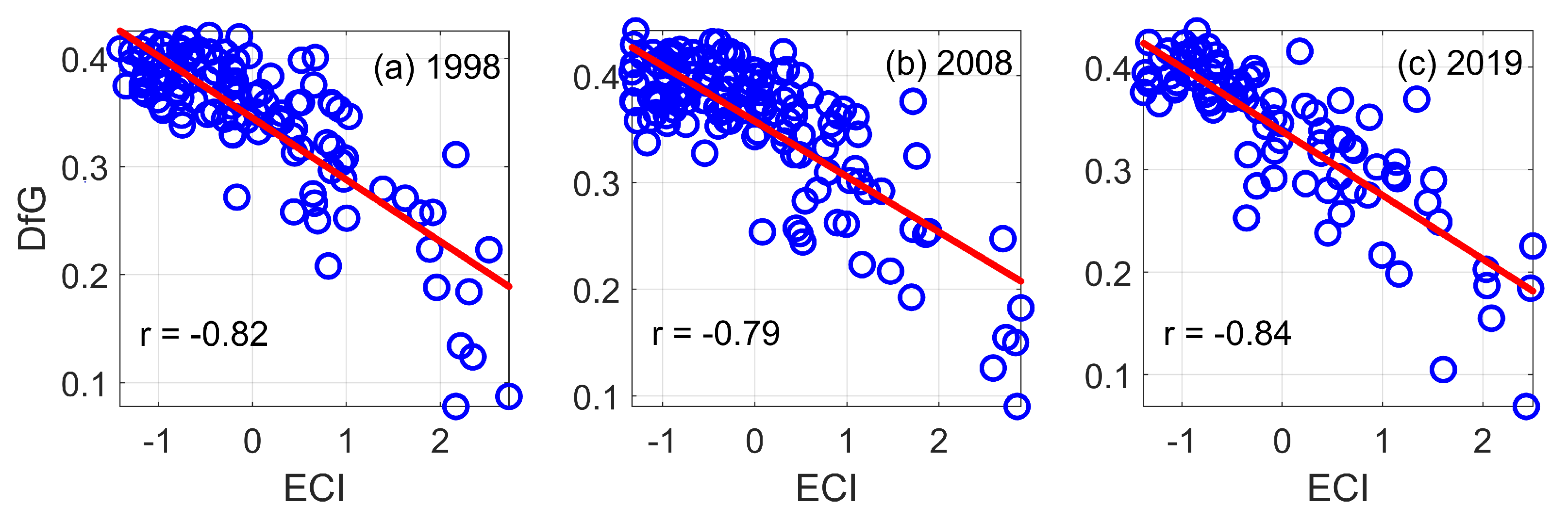
3.2. DfG and Economic Complexity

Considering that the level of DfG is closely related to specialization and division of labor, it is necessary to examine the connection between DfG and economic complexity. Figure 5a–c show correlations between DfG and ECI in 1998, 2008 and 2019, respectively. Clearly, we observe that the DfG is very strongly negatively correlated with the ECI. This suggests that the higher level of economic complexity, the smaller the DfG. In other words, the higher level of economic complexity, the closer a country’s RCA index to a normal distribution. Therefore, relationships between the DfG and economic development and economic complexity reflect that a closer a country’s RCA index to a normal distribution, the higher degree of economic complexity and better economic performance of a country.

It is interesting to compare the Pearson correlation coefficient between DfG and the logarithm of GDP and that between ECI and the logarithm of GDP. Since the correlation coefficient for the former is negative but positive for the latter, it is more convenient to use the Pearson correlation coefficient between DfG and the logarithm of GDP in absolute value. The result for the comparison is shown in Figure 6, where the red curve denotes the absolute value of the correlation coefficient between DfG and the logarithm of GDP, and the blue curve is for the correlation coefficient between ECI and the logarithm of GDP. We observe that before the global financial crisis of 2008, the correlation coefficients between DfG and the logarithm of GDP, and between ECI and the logarithm of GDP, are comparable. However, after the global financial crisis, the correlation coefficients between DfG and the logarithm of GDP are persistently larger than those between ECI and the logarithm of GDP. The significance of this feature for designing better indicators of economic complexity will be further discussed in the last section.

Out of curiocity, we have examined whether DfG using import data is still strongly negatively correlated with the logarithm of GDP. The answer is positive. In fact, the correlation coefficient using import data is basically identical to that using export data. This interesting property however, is not shared by ECI—when using import data, whether we focus on adjacency matrices based on RCA $\ge 1$ or RCA $<1$, the computed “ECI” essentially has no correlation with the logarithm of GDP. This signifies that RCA $\ge 1$ or RCA $<1$ based on import data cannot be interpretated as that based on export data to have comparative advantage or disadvantage.

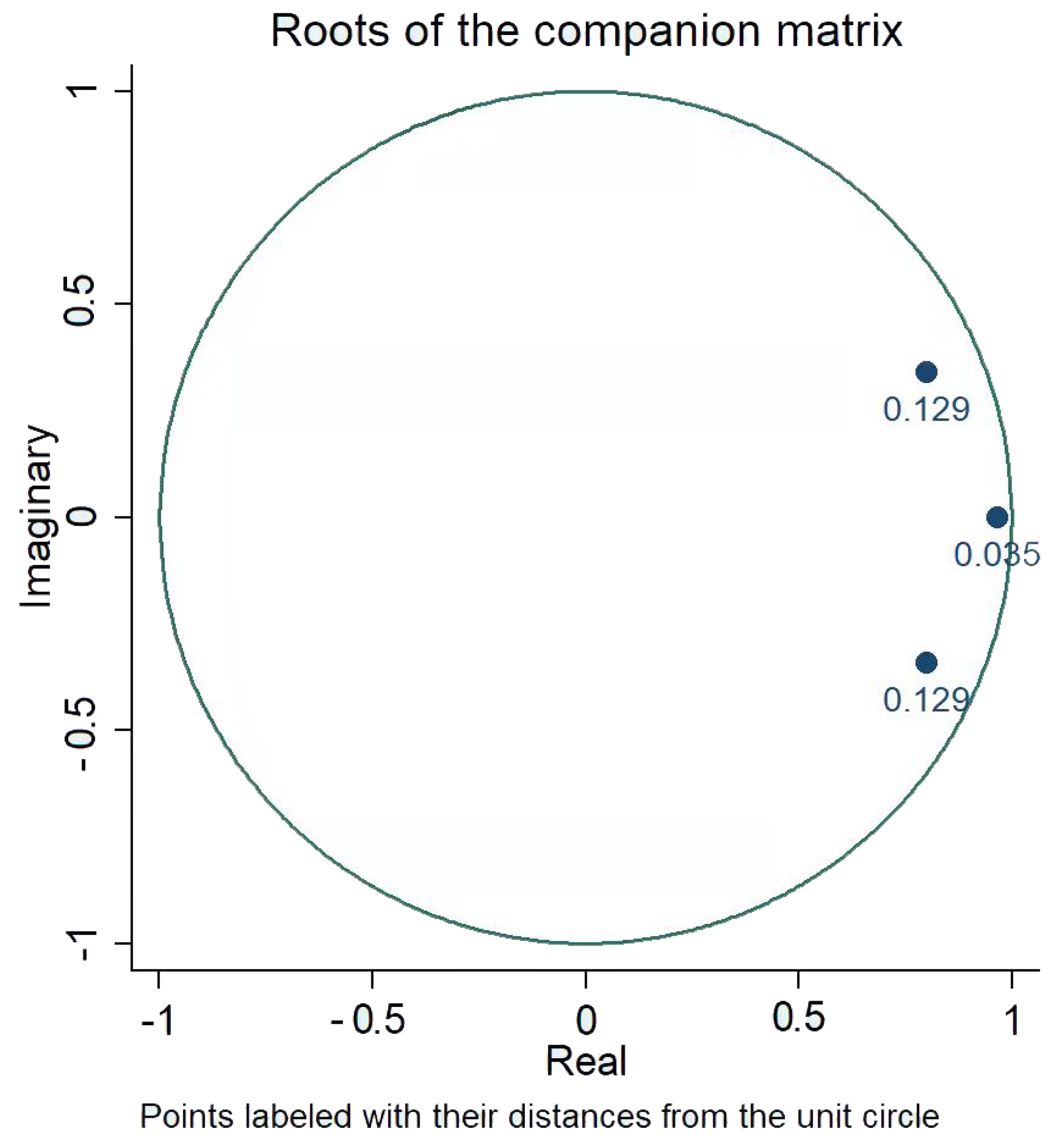
3.3. Regression and Causality Analysis

To understand more deeply the connection between DfG and economic development, we have employed the Pooled OLS model. The results are summarized in

Table 1. Regression results for GDP, DfG and ECI.

Variables	Model 1–3 (1996–2019)			Model 4–6 (1996–2007)			Model 7–9 (2008–2019)
	ln GDP	ln GDP	ln GDP	ln GDP	ln GDP	ln GDP	ln GDP	ln GDP	ln GDP
DfG	−18.97 ***${}^1$ (−43.95)		−15.04 *** (−21.29)	−19.78 *** (−33.74)		−13.65 *** (−14.34)	−18.48 *** (−33.05)		−16.88 *** (−14.34)
ECI		1.26 *** (34.78)	0.37 *** (6.95)		1.43 *** (29.2)	0.58 *** (7.98)		1.11 *** (22.73)	0.14 ** (2.16)
Constant	31.94 *** (221.73)	25.16 *** (593.36)	30.48 *** (120.6)	31.75 *** (163.24)	24.67 *** (442.62)	29.49 *** (86.8)	32.22 *** (171.91)	25.64 *** (437.45)	31.64 *** (96.43)
Observations	1440	1440	1440	720	720	720	720	720	720
Adjusted $R^2$	0.573	0.457	0.587	0.623	0.543	0.645	0.603	0.418	0.605
F-Statistics	1931.66	1209.56	1021.59	1138.19	852.59	650.51	1092.18	516.62	551.22
Prob > F	0.000	0.000	0.000	0.000	0.000	0.000	0.000	0.000	0.000

¹Note: *** p < 0.01, ** p < 0.05.

. Here, we select 60 countries which have continuous data from 1996 to 2019. We thus have a total of 1440 observations. We have first run a pooled OLS regression for the whole period. The results are shown in columns 1 to 3 of Table 1, where the 1st column is for the model with only DfG considered, the 2nd column for the results with only ECI considered, and the 3rd column for both DfG and ECI considered. We call these models 1–3. We observe that the regression coefficients for models 1–3 are significant at the 1% level. By comparing the columns 1 and 2, we find that DfG can explain 57.3 percent of the variance in GDP, while ECI accounts for 45.7 percent, as shown by the $R^2$ of the regression. This suggests that the explanatory power of DfG on GDP is stronger than that of ECI. After both DfG and ECI are considered, the model explains 58.7 percent of the variance in GDP, which is slightly better than model 1.

Considering that DfG has a higher correlation with GDP than ECI since the global financial crisis of 2008, we have also divided the whole time period into two, one from the year 1996 to 2007, the other from 2008 to 2019. The results are shown in the columns 4–6 and 7–9 of Table 1, for the models 1–3 explained earlier. By comparing the results of regression models for these two groups, we find: (1) in both time periods DfG has a stronger explanatory power on the variance of GDP than ECI, (2) the explanatory power of DfG and ECI coombined on the variance of GDP in first group is stronger that that of the second group. It is worth noting that ECI does not significantly improve the explanatory power of the model on the variance of GDP in these three scenarios of regression models, especially in the period after the global financial crisis of 2008. Therefore, DfG better explains the variance in GDP than ECI.

We have also performed a panel VAR analysis. LLC test indicates that the three variables with one period lag and trend are stationary. This allows us to estimate the coefficients of the system described by Equation (9) after the individual effects removed. Robustness test shows that the PVAR model is reasonable, as shown in Figure 7.

Table 2. Main results of a three-variables panel VAR.

Response of	Response to
	${\ln \mathrm{GDP}}_{(\mathrm{t}-1)}$	${\mathrm{DfG}}_{(\mathrm{t}-1)}$	${\mathrm{ECI}}_{(\mathrm{t}-1)}$
${\ln \mathrm{GDP}}_{\left(\mathbf{t}\right)}$	0.961 ***${}^1$ (130.16)	−0.313 (−1.40)	0.027 (0.6)
${\mathrm{DfG}}_{\left(\mathbf{t}\right)}$	−0.008 *** (−7.96)	0.734 *** (24.23)	0.027 *** (4.41)
${\mathrm{ECI}}_{\left(\mathbf{t}\right)}$	0.292 *** (15.10)	−4.864 *** (−8.31)	0.874 *** (7.43)
Observations	1440
N countries	60

¹Note: *** p < 0.01.

shows the results of the model with three variables, from the columns of which we find that the impact of $ln\mathrm{GDP}$ with one period lag on $ln\mathrm{GDP}$, DfG and ECI are significant for all three different panel VARs, the impact of DfG with one period lag on DfG and ECI are significant, and the impact of ECI with one period lag on DfG and ECI are significant. However, impacts of DfG and ECI with one period lag on ln GDP are not significant. On the other hand, impact of DfG with one period lag on DfG is positive but negative on ECI, while the impacts of ECI with one period lag on both DfG and ECI are positive.

Finally, we have examined the statistical causality among the three variables based on PVAR by using panel Granger causality Wald test. The results are shown in

Table 3. Granger causality Wald tests for Panel VAR.

Hypothesis	chi2	df	Prob >  chi2
ln GDP does not Granger cause DfG	1.971	1	0.160
ln GDP does not Granger cause ECI	0.365	1	0.546
DfG does not Granger cause ln GDP	63.338	1	0.000 ***${}^1$
DfG does not Granger cause ECI	19.434	1	0.000 ***
ECI does not Granger cause ln GDP	227.91	1	0.000 ***
ECI does not Granger cause DfG	69.104	1	0.000 ***

¹Note: *** p < 0.01.

. We observe that the $ln\mathrm{GDP}$ is not the Granger cause of DfG and ECI at the 5% level, while the DfG and ECI are the Granger cause of $ln\mathrm{GDP}$ at the 1% level. This result is as anticipated.

4. Discussion

Understanding the difference in economic development among countries or regions is a long-standing issue in economics. A crucial perspective to shed light on the issue is to evaluate competitiveness of a country in international trade as characterized by the RCA index. Although it is desirable to have a normally distributed RCA, empirical studies have often found the opposite. This discrepancy has stimulated a lot of researchers to develop alternative indices of the RCA index so that their distributions would be closer to Gaussian distributions. Yet, those efforts are not very successful. This calls for a deeper understanding of the significance of a normally distributed RCA index.

To gain insights into this issue, we have defined a quantity, DfG, based on the KS test, which quantifies the deviation of the distribution of a country’s RCA index from normality. We have found that the variations of DfG are characterized by spatiotemporal heterogeneity and regional spatial agglomeration. The spatiotemporal heterogeneity of the DfG refers to the significant differences in many countries’ DfG and their dynamic evolution. Regional spatial agglomeration of the DfG refers to that countries with smaller DfG are mainly concentrated in North America (represented by USA), Western Europe (represented by Germany), and Eastern Asia (represented by China, Japan and South Korea). Interestingly, these three areas are very consistent with the description of “The world seems to have three interconnected production hubs for the extensive trade in parts and components” in the “Global Value Chain Development Report 2017—Measuring and Analyzing the Impact of GVCs on Economic Development”. It suggests that the DfG has some connections with the development of GVCs. On the other hand, countries with larger DfG are mainly concentrated in Africa, South America, Western and Southern Asia.

The pattern of DfG’s spatial variation suggests that the DfG can act as a good indicator of a country’s economic performance. This is indeed so, as DfG is found to be strongly negatively related with both the logarithm of GDP and the ECI. Therefore, the closer the distribution of a country’s RCA index to a normal distribution, the higher degree of economic complexity and better economic performance of the country. This highlights the optimality of a country’s export when its RCA index follows a normal distribution, and provides a new perspective to understand the difference in economic development among countries or regions. Furthermore, we have found that the correlation coefficients between DfG and the logarithm of GDP are persistently larger than those between ECI and the logarithm of GDP after the 2008 global financial crisis. This is further corroborated by regression analysis which shows that DfG better explains the variance in GDP than ECI. Further Granger causality analysis shows that DfG and ECI are the Granger cause of $ln\mathrm{GDP}$, but not the vice versa. It is worth emphasizing that Gaussianity is not a cause, it is more a consequence indicating economic development.

The last feature, that DfG is more strongly correlated with GDP than ECI, suggests an interesting way to improve characterization of economic complexity of a country. For this purpose, we need to first understand the meaning of the correlation between ECI and the logarithm of GDP. This is due to the strong correlation between export and GDP—ECI amounts to retaining only products with RCA equal to or greater than 1 and approximating the amount of export by counting the number of products with RCA $\ge 1$. Our observation that after the 2008 global financial crisis, the correlation between DfG and GDP is stronger than that between ECI and GDP, can at least be partially attributed to the enhancement of the global participation in production chains, or simply, greater participation in global value chains (GVCs). Therefore, simply focusing on RCA $\ge 1$, which has been used in designing ECI and its variants, is no longer sufficient. In other words, information contained in products with RCA $<1$ can no longer be simply discarded. Therefore, in future, it would be extremely interesting to develop a new economic complexity index by using DfG alone, or by combining DfG and ECI (or its variants).

References

1. Balassa, B. Trade liberalization and ‘revealed’ comparative advantage. Manch. Sch. Econ. Soc. Stud. 1965, 32, 99–123. [Google Scholar] [CrossRef]
2. Yeats, A.J. On the Appropriate Interpretation of the Revealed Comparative Advantage Index: Implications of a Methodology based on Industry Sector Analysis. Weltwirtsch. Arch. 1985, 121, 61–73. [Google Scholar] [CrossRef]
3. Leromain, E.; Orefice, G. New revealed comparative advantage index: Dataset and empirical distribution. Int. Econ. 2014, 139, 48–70. [Google Scholar] [CrossRef]
4. Hoen, A.R.; Oosterhaven, J. On the measurement of comparative advantage. Ann. Reg. Sci. 2006, 40, 677–691. [Google Scholar] [CrossRef] [Green Version]
5. Yu, R.; Cai, J.; Leung, P. The normalized revealed comparative advantage index. Ann. Reg. Sci. 2009, 43, 267–282. [Google Scholar] [CrossRef]
6. Hinloopen, J.; Marrewijk, C.V. On the empirical distribution of the Balassa index. Weltwirtsch. Arch. 2001, 137, 1–35. [Google Scholar] [CrossRef] [Green Version]
7. De Benedictis, L.; Tamberi, M. Overall specialization empirics: Techniques and applications. Open Econ. Rev. 2004, 15, 323–346. [Google Scholar] [CrossRef]
8. Bowen, H.P. On the Theoretical Interpretation of Indices of Trade Intensity and Revealed Comparative Advantage. Weltwirtsch. Arch. 1983, 119, 464–472. [Google Scholar] [CrossRef]
9. Laursen, K. Revealed comparative advantage and the alternatives as measures of international specialization. Eurasian Bus. Rev. 2015, 5, 99–115. [Google Scholar] [CrossRef]
10. Deb, K.; Sengupta, B. On empirical distribution of RCA Indices. IIM Kozhikode Soc. Manag. Rev. 2017, 6, 23–41. [Google Scholar] [CrossRef] [Green Version]
11. Vollrath, T.L. A Theoretical Evaluation of Alternative Trade Intensity Measures of Revealed Comparative Advantage. Weltwirtsch. Arch. 1991, 127, 265–280. [Google Scholar] [CrossRef]
12. Dalum, B.; Laursen, K.; Villumsen, G. Structural change in OECD export specialisation patterns: De-specialisation and ‘stickiness’. Int. Rev. Appl. Econ. 1998, 12, 423–443. [Google Scholar] [CrossRef]
13. Proudman, J.; Redding, S. Evolving patterns of international trade. Rev. Int. Econ. 2000, 8, 373–396. [Google Scholar] [CrossRef] [Green Version]
14. Amador, J.; Cabral, S.; Maria, J.R. A simple cross-country index of trade specialization. Open Econ. Rev. 2011, 22, 447–461. [Google Scholar] [CrossRef]
15. Jenny, P.D.B.; Rémi, S. A New Class of Revealed Comparative Advantage Indexes. Open Econ. Rev. 2021, 1–27. [Google Scholar] [CrossRef]
16. Liu, B.; Gao, J.B. Understanding the non-Gaussian distribution of revealed comparative advantage index and its alternatives. Int. Econ. 2019, 158, 1–11. [Google Scholar] [CrossRef]
17. Hidalgo, C.A.; Klinger, B.; Barabási, A.L.; Hausmann, R. The product space conditions the development of nations. Science 2007, 317, 482–487. [Google Scholar] [CrossRef] [PubMed] [Green Version]
18. Hidalgo, C.; Hausmann, R. The building blocks of economic complexity. Proc. Natl. Acad. Sci. USA 2009, 106, 10570–10575. [Google Scholar] [CrossRef] [PubMed] [Green Version]
19. Mealy, P.; Farmer, J.D.; Teytelboym, A. Interpreting economic complexity. Sci. Adv. 2019, 5, 1–8. [Google Scholar] [CrossRef] [PubMed] [Green Version]
20. Andrea, T.; Mazzilli, D.; Pietronero, L. A dynamical systems approach to gross domestic product forecasting. Nat. Phys. 2018, 14, 861–865. [Google Scholar]
21. Gao, J.; Zhang, Y.C.; Zhou, T. Computational socioeconomics. Phys. Rep. 2019, 817, 1–104. [Google Scholar] [CrossRef] [Green Version]
22. Tacchella, A.; Cristelli, M.; Caldarelli, G.; Gabrielli, A.; Pietronero, L. A new metrics for countries’ fitness and products’ complexity. Sci. Rep. 2012, 2, 723. [Google Scholar] [CrossRef] [PubMed] [Green Version]
23. Tacchella, A.; Cristelli, M.; Caldarelli, G.; Gabrielli, A.; Pietronero, L. Economic complexity: Conceptual grounding of a new metrics for global competitiveness. J. Econ. Dynam. Control 2013, 37, 1683–1691. [Google Scholar] [CrossRef]
24. Caldarelli, G.; Cristelli, M.; Gabrielli, A.; Pietronero, L.; Scala, A.; Tacchella, A. A network analysis of countries’ export flows: Firm grounds for the building blocks of the economy. PLoS ONE 2012, 7, e47278. [Google Scholar] [CrossRef] [PubMed] [Green Version]
25. Cristelli, M.; Gabrielli, A.; Tacchella, A.; Caldarelli, G.; Pietronero, L. Measuring the intangibles: A metrics for the economic complexity of countries and products. PLoS ONE 2013, 8, e70726. [Google Scholar] [CrossRef] [Green Version]
26. Battiston, F.; Cristelli, M.; Tacchella, A.; Pietronero, L. How metrics for economic complexity are affected by noise. Complex. Econ. 2014, 3, 1–22. [Google Scholar]
27. Mariani, M.S.; Vidmer, A.; Medo, M.; Zhang, Y.C. Measuring economic complexity of countries and products: Which metric to use? Eur. Phys. J. B 2015, 88, 293. [Google Scholar] [CrossRef]
28. Wu, R.J.; Shi, G.Y.; Zhang, Y.C.; SebastianMariani, M. The mathematics of non-linear metrics for nested networks. Phys. A 2016, 460, 254–269. [Google Scholar] [CrossRef] [Green Version]
29. Felipe, J.; Kumar, U.; Abdon, A.; Bacate, M. Product complexity and economic development. Struct. Chang. Econ. Dyn. 2012, 23, 36–68. [Google Scholar] [CrossRef] [Green Version]
30. Poncet, S.; Waldemar, F.S.D. Export upgrading and growth: The prerequisite of domestic embeddedness. World Dev. 2013, 51, 104–118. [Google Scholar] [CrossRef] [Green Version]
31. Hausmann, R.; Hidalgo, C. The Atlas of Economic Complexity: Mapping Paths to Prosperity; MIT Press: Cambridge, MA, USA, 2014. [Google Scholar]
32. Zhu, S.; Yu, C.; He, C. Export structures, income inequality and urban-rural divide in China. Appl. Geogr. 2020, 115, 102150. [Google Scholar] [CrossRef]
33. Neagu, O.; Teodoru, M.C. The relationship between economic complexity, energy consumption structure and greenhouse gas emission: Heterogeneous panel evidence from the EU countries. Sustainability 2019, 11, 497. [Google Scholar] [CrossRef] [Green Version]
34. Romero, J.P.; Gramkow, C. Economic complexity and greenhouse gas emissions. World Dev. 2021, 139, 105317. [Google Scholar] [CrossRef]
35. Lapatinas, A. Economic complexity and human development: A note. Econ. Bull. 2016, 366, 1441–1452. [Google Scholar]
36. Vu, T.V. Economic complexity and health outcomes: A global perspective. Soc. Sci. Med. 2020, 265, 113480. [Google Scholar] [CrossRef] [PubMed]
37. Hartmann, D.; Guevara, M.R.; Jara-Figueroa, C.; Manuel, A.; Hidalgo, C.A. Linking economic complexity, institutions, and income inequality. World Dev. 2017, 93, 75–93. [Google Scholar] [CrossRef] [Green Version]
38. Chavez, J.C.; Marco, T.M.; Manuel, G.Z. Economic complexity and regional growth performance: Evidence from the Mexican Economy. Rev. Reg. Stud. 2017, 47, 201–219. [Google Scholar] [CrossRef]
39. Gao, J.; Zhou, T. Quantifying China’s regional economic complexity. Phys. A Stat. Mech. Its Appl. 2018, 492, 1591–1603. [Google Scholar] [CrossRef] [Green Version]
40. Fritz, B.S.; Robert, A.M. The economic complexity of US metropolitan areas. Reg. Stud. 2021, 1–12. [Google Scholar] [CrossRef]
41. Hidalgo, C.A. Economic complexity theory and applications. Nat. Rev. Phys. 2021, 3, 92–113. [Google Scholar] [CrossRef]
42. Stojkoski, V.; Utkovski, Z.; Kocarev, L. The impact of services on economic complexity: Service sophistication as route for economic growth. PLoS ONE 2016, 11, e0161633. [Google Scholar] [CrossRef] [PubMed] [Green Version]
43. Wooldridge, J.M. Selection corrections for panel data models under conditional mean independence assumptions. J. Econom. 1995, 68, 115–132. [Google Scholar] [CrossRef]
44. Wooldridge, J.M. Econometric Analysis of Cross Section and Panel Data; MIT Press: Cambridge, MA, USA, 2010. [Google Scholar]
45. Love, I.; Zicchino, L. Financial development and dynamic investment behavior: Evidence from panel VAR. Q. Rev. Econ. Financ. 2006, 46, 190–210. [Google Scholar] [CrossRef]
46. Koutsomanoli-Filippaki, A.; Mamatzakis, E. Performance and Merton-type default risk of listed banks in the EU: A panel VAR approach. J. Bank. Financ. 2009, 33, 2050–2061. [Google Scholar] [CrossRef] [Green Version]
47. Levin, A.; Lin, C.F.; Chu, C.S.J. Unit root tests in panel data: Asymptotic and finite-sample properties. J. Econom. 2002, 108, 1–24. [Google Scholar] [CrossRef]
Figure 1. The distribution features of the two parts of RCA index (a,b) and the Probability Distribution Function (PDF) of RCA index (c,d) for Germany and Japan under the HS4 scheme in 2018.
Applsci 12 01125 g001
Figure 2. Spatial variations of the DfG in 1998, 2008 and 2018 under the HS4 scheme.
Applsci 12 01125 g002
Figure 3. Regression analysis showing correlation between DfG and the logarithm of GDP in 1998, 2008 and 2019.
Applsci 12 01125 g003
Figure 4. Dynamic evolution of the DfG for China, India, Australia and Zambia from 1991 to 2019 under the HS4 scheme.
Applsci 12 01125 g004
Figure 5. Regression analysis showing correlation between DfG and ECI in 1998, 2008 and 2019.
Applsci 12 01125 g005
Figure 6. Variation of the Pearson correlation with time, where the red and the blue curves are for the absolute value of the correlation coefficient between DfG and the logarithm of GDP, and the correlation coefficient between ECI and the logarithm of GDP.
Applsci 12 01125 g006
Figure 7. Robustness test of Panel VAR.
Applsci 12 01125 g007