Visual Sentiment Analysis Using Deep Learning Models with Social Media Data

Abstract

Analyzing the sentiments of people from social media content through text, speech, and images is becoming vital in a variety of applications. Many existing research studies on sentiment analysis rely on textual data, and similar to the sharing of text, users of social media share more photographs and videos. Compared to text, images are said to exhibit the sentiments in a much better way. So, there is an urge to build a sentiment analysis model based on images from social media. In our work, we employed different transfer learning models, including the VGG-19, ResNet50V2, and DenseNet-121 models, to perform sentiment analysis based on images. They were fine-tuned by freezing and unfreezing some of the layers, and their performance was boosted by applying regularization techniques. We used the Twitter-based images available in the Crowdflower dataset, which contains URLs of images with their sentiment polarities. Our work also presents a comparative analysis of these pre-trained models in the prediction of image sentiments on our dataset. The accuracies of our fine-tuned transfer learning models involving VGG-19, ResNet50V2, and DenseNet-121 are 0.73, 0.75, and 0.89, respectively. When compared to previous attempts at visual sentiment analysis, which used a variety of machine and deep learning techniques, our model had an improved accuracy by about 5% to 10%. According to the findings, the fine-tuned DenseNet-121 model outperformed the VGG-19 and ResNet50V2 models in image sentiment prediction.

1. Introduction

The concept of human–computer interaction is the need of the hour and has tremendous applications [1]. It involves the use of machines/computers to make decisions and to predict certain things such as sentiments. It employs some artificial intelligence techniques to implement sentiment analysis on images. Facebook and YouTube are very popular among Americans and they post a lot of text/images [2]. The authors have also found that the use of social media sites, such as Instagram, Pinterest, and WhatsApp, is very common among adults younger than 30 years of age. The unprocessed social media records can be converted into a useful form and processed to benefit several business-related applications [3]. The concept of sentiment analysis is an important branch of natural language processing (NLP), and it is vital to understand the opinion of the people in many applications [4,5,6]. Customer reviews [7], film reviews [8], hotel reviews [9], and social media monitoring [10] are all common uses of it. Sentiment analysis involves the classification of sentiments of people into different categories, such as positive, negative, and neutral [11]. The main problem in text-based sentiment analysis involves the presence of multilingual data, and complex text cannot be understood by all compared to images. The visual content attracts social media users more compared to text. Some of the social media sites, such as Flickr and Instagram, give importance to image posts rather than textual posts [12]. To analyze the sentiment from images, we need intelligent approaches, and a lot of effort is to be involved. Visual sentiment prediction models involve the finding of sentiment polarity (positive, negative, and neutral) associated with the given image. There are different ways in which visual sentiment analysis can be done, but the use of pre-trained deep learning models can increase the performance of sentiment classification tasks even with imbalanced datasets [13]. The transfer learning models, when used for classification, yield better results compared to machine learning models for the same task [14,15,16]. In our work, we used the existing pre-trained transfer learning models, including the VGG-19, DenseNet-121, and ResNet50V2 models, for image sentiment prediction on the Crowdflower sentiment polarity dataset. The following are our primary contributions.

• We introduced a unique approach that uses fine-tuned transfer learning models to handle the issues of image sentiment analysis.
• To mitigate overfitting, we employed additional layers, such as dropout and weight regularization (L1 and L2 regularization). By performing a grid search across several values of the regularization parameter, we were able to find the value that gives the model its maximum accuracy.
• On a typical dataset, we show that a visual sentiment analysis approach comprising fine-tuned DenseNet-121 architecture outperforms the previous state-of-the-art model.

The rest of the paper is structured as follows: Section 2 discusses some of the existing work on image sentiment analysis using various methods. Section 3 presents a block diagram that explains the steps in determining the image polarity. In Section 4, the methodology involving the transfer learning concept with the architectural details is presented. In Section 5, the information about the dataset and some sample images are shown. In Section 6, the experimental results are shown in terms of some performance metrics, such as precision, accuracy, F1 score, and so on. This section also discusses the comparative analysis of the various pre-trained models. In Section 7, the conclusion of our work is presented with the future scope.

2. Literature Survey

In this section, we go through some of the existing research on image sentiment prediction that has been done. Image sentiment analysis is done by using any one of the following approaches involving the extraction of low-level features, semantic features, and with machine and deep learning models. The pixel-level features, along with some low-level features, such as color and texture, were used in [17] to predict image sentiments. The authors of [18] used the Bag-of-Visual-Words (BoVW) technique with latent semantic analysis (LSA) to classify the image emotions. They addressed the challenge of capturing emotion types present in different regions of an image. The authors of [19,20] extracted aesthetic features from the images that are related to beauty or art to perform visual sentiment analysis and achieved significant results compared to low-level features.

The concept of adjective–noun pairs (ANPs) was proposed by [21] to describe the emotional/sentiment details of images. They also developed an approach known as SentiBank to identify 1200 ANP present in images. The authors of [22] developed a mid-level attribute known as Sentribute as an alternative to low-level attributes to classify visual sentiments. They were able to establish an association between these attributes and the emotional sentiments evoked by the images. The ANPs were used by the authors of [23] in their work to extract image features with a support vector machine (SVM) classifier for sentiment classification. They were able to achieve a precision of 0.86 on the visual sentiment ontology (VSO) dataset containing 603 images on various topics. ANPs, which are also known as mid-level descriptors of images, were used for automatic emotion and sentiment finding from images by the authors of [24]. They were able to attain better results compared to low-level image descriptors and the use of ANPs helped to determine the sentiment/emotional information.

The concept of deep coupled adjective and noun neural networks was used by the researchers of [25] in their work to overcome some of the challenges in analyzing the sentiment of images. They were able to accomplish better results by combining the convolutional neural network (CNN) with separate adjective and noun networks. The authors of [26] used some local regions and entire images that have sentiment information with the convolutional neural network (CNN) to obtain sentiment scores. An architecture combining the CNN with a visual attention model was proposed by the authors of [27] to determine the image sentiments of the Twitter and ART photo datasets. Another work on image sentiment analysis by the researchers of [28] extracted objective text descriptions from the images, and they trained a support vector machine (SVM) classifier to determine the sentiment polarity. They used a dataset with 47235 images and were able to achieve an accuracy of 73.96 combining text and visual features. The authors of [29] built a deep-learning-based long short-term memory model (LSTM) to do image sentiment analysis on Flickr images and Twitter datasets. They achieved an accuracy of 0.84 on Flickr and of 0.75 on the Twitter datasets. The authors of [30] joined the semantic and visual features for image sentiment analysis, which yielded better results.

Table 1. Existing works on visual sentiment prediction based on low, mid, and deep visual features.

S. No.	Author Name	Technique Used and Results	Merits	Limitations
1	Tao Chen et al. [31]	Adjective–noun pairs (ANP) and convolutional neural networks (CNN) trained based on Caffe. The proposed DeepSentibank outperformed SentiBank 1.1 by 62.3%.	The suggested model enhances annotation accuracy as well as ANP retrieval performance.	To reduce overfitting, network structure must be adjusted.
2	V’ıctor Camposa et al. [32]	Fine-tuned CaffeNet CNN architecture was employed. Obtained an accuracy of 0.83 on Twitter dataset for sentiment prediction.	The model uses fewer training parameters and provides a robust model for sentiment visualization.	To accommodate the presence of noisy labels, the architecture must be rebuilt.
3	Jana Machajdik et al. [33]	Low-level visual features based on psychology were applied. Accuracy rates of more than 70% were obtained for classifying a variety of emotions.	Able to generate an emotional histogram displaying the distribution of emotions across multiple categories.	To improve the outcomes, more and better features are required.
4	Marie Katsurai et al. [34]	RGB histograms, GIST descriptors, and mid-level features were employed as visual descriptors. On the Flickr dataset, the proposed model achieved an accuracy of 74.77%.	Multi-view (text + visual) embedding space is effective in classifying visual sentiment.	Investigation is needed regarding features to improve the system performance.
5	Yilin Wang et al. [35]	Unsupervised sentiment analysis framework (USEA) was proposed. Achieved an accuracy score of 59.94% for visual sentiment prediction on Flickr dataset.	The “semanticgap” between low- and high-level visual aspects was successfully resolved.	More social media sources, such as geo-location and user history, must be examined in order to boost performance even more.

, below, covers some of the existing works on visual sentiment prediction based on low, mid, and deep visual features.

The drawbacks found in existing works on visual sentiment analysis can be eliminated by employing fine-tuned transfer learning models that are trained on a large set of data. The transfer learning models are suitable for sentiment analysis and other natural language processing tasks [36,37,38] and provide many advantages compared to other conventional models. We used three different transfer learning models—the VGG-19, DenseNet-121, and ResNet50V2 models—for visual sentiment prediction from the Crowdflower dataset. The deep learning method’s performance is dependent on huge data support. When obtaining a high number of labeled data samples is challenging, the efficacy of the learning algorithm suffers. When there is not enough data, the developed deep learning network structure is susceptible to overfitting [39]. Transfer learning, which involves applying knowledge or patterns learned in one field or activity to distinct but related disciplines or challenges, can effectively tackle the problem of limited training data in the appropriate field [40]. As a result, we used the transfer learning strategy for image sentiment polarity with much fewer training examples (1000 image samples) to prevent overfitting and to optimize system performance. To initialize the hyperparameters of our network, we used transfer learning and weights and biases from a pre-trained ImageNet model. With the help of extra layers, such as drop-out and regularization layers (L1 and L2 regularization), we were able to reduce overfitting in our network and increase the system performance. Our system outperformed other systems in visual sentiment analysis.

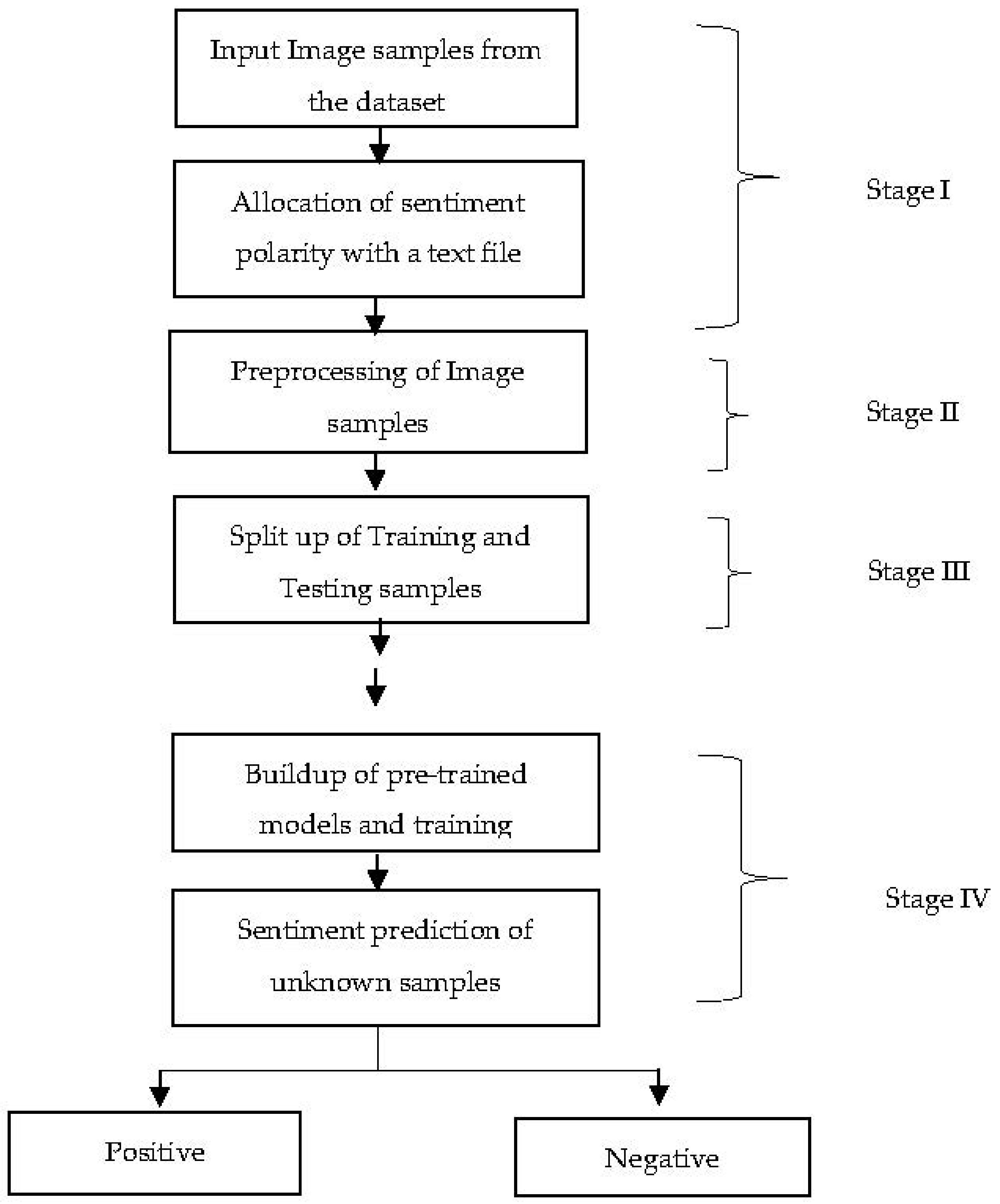
3. The Proposed Work—Block Diagram

The effectiveness of our model in predicting sentiments using a fine-tuned transfer learning model is shown in Figure 1. This was done by fine-tuning the existing pre-trained VGG-19, ResNet50V2, and DenseNet-121 models. The reason for choosing the ResNet50V2 model is that it can reduce the vanishing gradient problem that happens when gradients are backpropagated, and the presence of residual or skip connection improves the learning [41]. It employs an identity connection or skip connection to increase system performance by lowering the error rate and uses a batch normalization layer before weight layers to improve classification performance. The DenseNet-121 model is favored by us because it can mitigate the vanishing gradient problem, requires fewer parameters, and has feature reuse capabilities. The validation error for the DenseNet model is much lower than that of the ResNet model, and the authors of [42] claim that DenseNet performed better based on extensive hyperparameter adjustments. We favor the VGG-19 model since it is an upgraded version of the VGG-16 model and is favored by many researchers for image classification tasks. Our work involved four stages— Stage I, Stage II, Stage III, and Stage IV. In Stage I, the image samples that were extracted from the Crowdflower dataset were loaded with their sentiment labels, which were available in a text file. We extracted about 1000 images from the dataset using the URLs of the images along with their sentiment polarity labels. In Stage II, the pre-processing of images was done by converting the images into an RGB format, and the resizing of the images into different dimensions was performed as required by the pre-trained models. The models required an image dimension of 224 × 224 × 3, and the normalization of image pixels was done in the next step. In Stage III, the training and testing samples were created by dividing the input image samples (1000) into training (795) and testing (205) images. Nearly 80% of the samples were utilized for training, with the remaining 20% being used for testing. In Stage IV, the training process was started by building the pre-trained model architectures with additional layers, and the prediction of unknown samples was done next. The fine-tuning of the models was done by freezing some layers and unfreezing the remaining layers. The performance metrics of the models, such as accuracy, precision, recall, and F1 measures, were generated, and the comparative analysis of the different pre-trained models was done.

4. Methodology

In this section, the need for the transfer learning concept is discussed, and the architecture of the different pre-trained models that we employed for image sentiment prediction is presented.

4.1. Transfer Learning

Transfer learning is one of the deep learning approaches that has lately been employed to solve complex challenges in NLP and computer vision. It improves the classification model’s performance by reducing computation time and increasing speed by using deep layers. It uses a model that has been trained on a known task to do a comparable task. It involves an optimization process in which the information gained from addressing a previous problem is transferred to a new challenge. Many pre-trained transfer learning-based models are available, each of which has been trained on a massive dataset containing millions of photos. The VGG-19, DenseNet, and ResNet models are popular, and they have been trained on the ImageNet dataset [43].

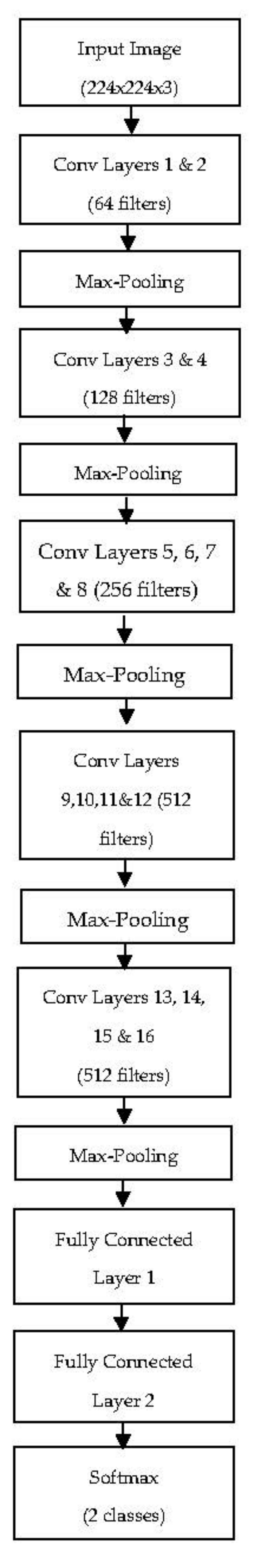
4.2. VGG-19 Architecture

The VGG-19 architecture comes with 19 weight layers, and the number of filters available in each layer doubles as we go deeper into the network. It has a stack of convolutional layers, followed by a max-pooling layer that extracts image features, and in the classification part, it has three fully connected layers and a Softmax layer. We trained our dataset on the VGG-19 architecture by fine-tuning it by freezing the first three convolutional blocks (Block 1, Block 2, and Block 3) and training the remaining layers (Block 4 and Block 5) that could extract features specific to our dataset. We added some additional layers in the classification part, that is, the flattening layer, batch normalization layer, dropout layer, and final dense layers, with 2 classes (positive and negative). The architecture of the VGG-19 model is shown in Figure 2 below.

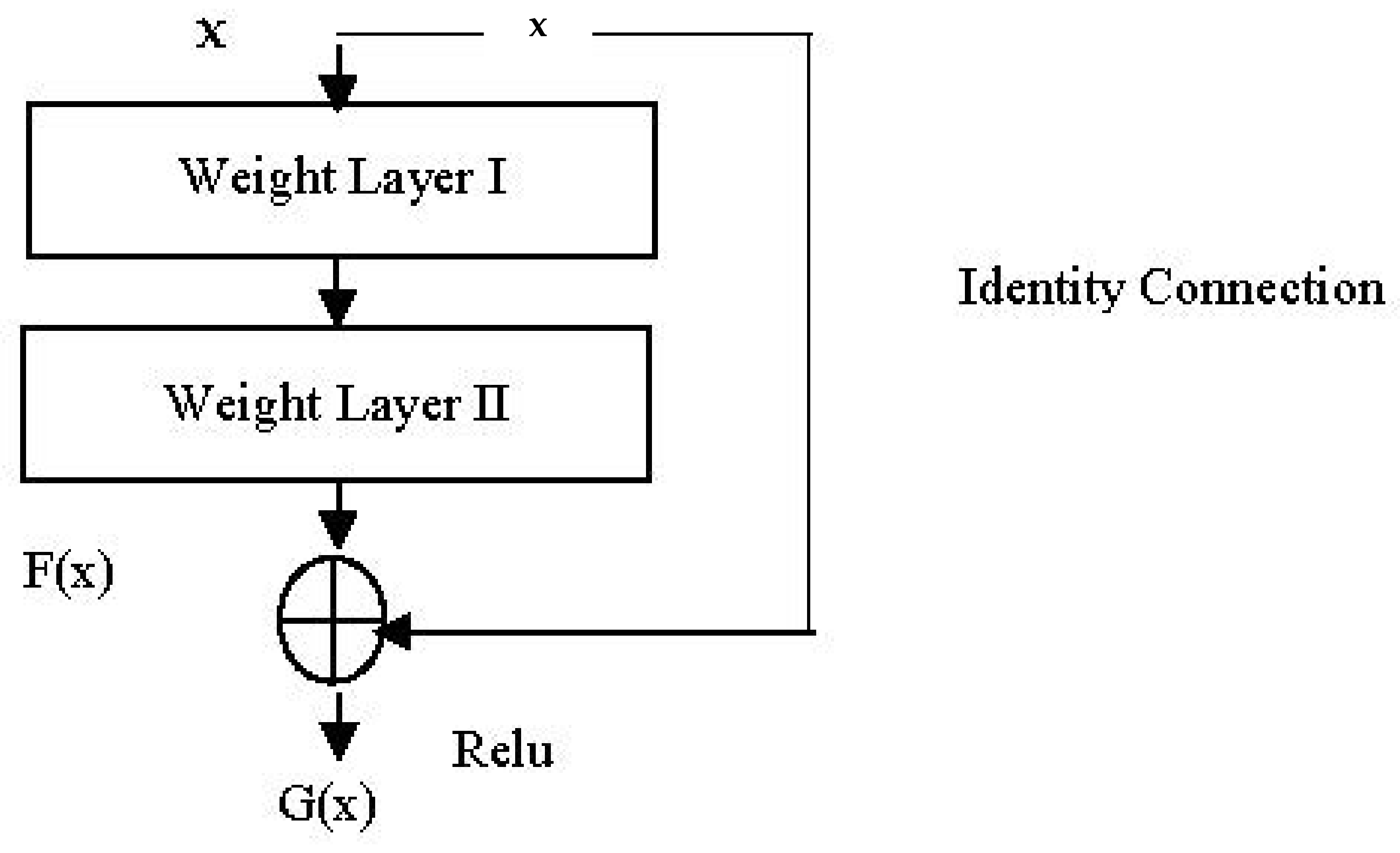
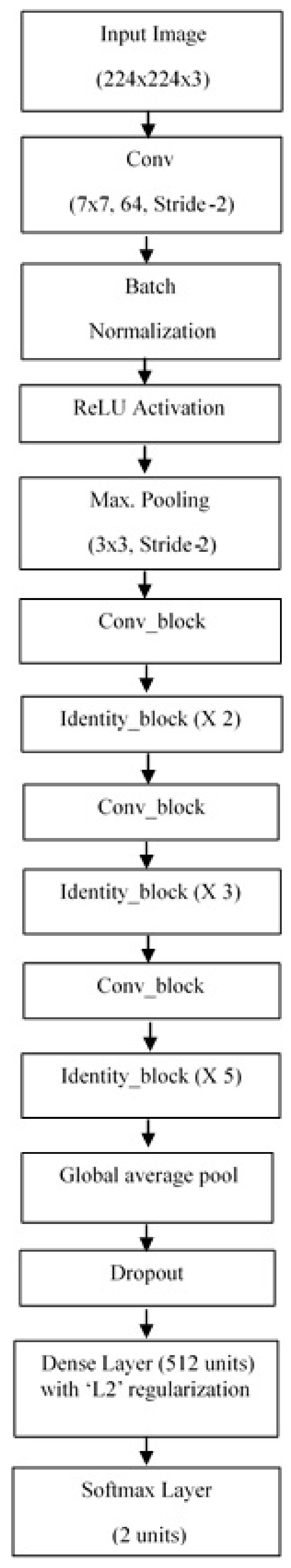
4.3. ResNet50V2 Architecture

The ResNet (Residual Networks (ResNet) deep neural networks were successfully used to solve image classification problems (ILSVRC 2015), and they outperformed the other deep neural architectures to get first prize in the competition. There are many ResNet architectures available that come up with different numbers of deep layers, such as ResNet-18, ResNet-50, ResNet-101, ResNet-151, and so on. The number that follows ResNet indicates the number of layers available in that network architecture.

Concept of Residual Network

The residual network’s purpose is to solve the problem of vanishing gradients that occurs during the training of a deep neural network with several layers. When the error is backpropagated and the gradient is computed during the training process, the gradient value decreases dramatically once the early layers are reached. The weight updation becomes very modest, to the point where the original weights are nearly identical to the updated weights gained from backpropagation. This adds the network’s input to the output of the convolutional block with weight layers through a connection known as an “identity connection” or “skip connection”. The concept of identity/skip connection in the residual network is shown in Figure 3.

Figure 3. Residual Network with identity connection.

Figure 3. Residual Network with identity connection.

G(x) = ReLU (x + F(x))

(1)

where

x is the input of the residual block with weight layers I and II;

G(x) is the output of the residual block;

F(x) is the output of the stacked convolutional or weight layers I and II.

The output function is represented as

$$\mathrm{y}=\mathrm{F}(\mathrm{x}, \{w_j\})+\mathrm{x}$$

(2)

where

F(x, $\left\{w_j\right\})$ denotes the residual block;

$w_j$ represents the weight layers ($w_1$ and $w_2$).

The dimensions of the input “x” and the output “F (x)” of the stacked convolutional layers I and II should be the same before adding them. If the dimensions are not the same, zeros can be added, that is, zero padding can be done. The inclusion of “identity connection” helps in overcoming the problem of vanishing gradients by providing a short path for the gradient. The following table (

Table 2. Layers in Resnet50V2 architecture.

Name of the Layer	Size of the Output	Resnet50V2
Conv 1 (Stage I)	112 × 112	7 × 7 convolution with a stride of 2
	112 × 112	3 × 3 max pooling with a stride of 2
Conv 2 (Stage II)	56 × 56	[1 × 1,64; 3 × 3,64 and 1 × 1,256] × 3
Conv 3 (Stage III)	28 × 28	[1 × 1,128; 3 × 3,128 and 1 × 1,512] × 4
Conv 4 (Stage IV)	14 × 14	[1 × 1,256; 3 × 3,256 and 1 × 1,1024] × 6
Conv 5 (Stage V)	7 × 7	[1 × 1,512; 3 × 3,512 and 1 × 1,2048] × 3
Classification	1 × 1	Global average pooling [7 × 7] with 1000 fully connected Softmax layers

) summarizes the different layers present in the basic Resnet50V2 model.

The ResNet50V2 model accepts 224 × 224 × 3 pixel input images. On input images, it first performs the convolution (7 × 7) and max-pooling (3 × 3) operations. There are four stages in this model, as well as some residual and identity blocks. For instance, in Stage I, the network provides three residual blocks (each with three layers) that conduct convolution operations with kernel sizes of 64 and 128. The size (width and height) of the input images are cut in half as it progresses through the phases, and the width of the image channel is doubled. The key difference between the ResNetV2 and ResNetV1 versions is that the former one does the convolution operation later, that is, after performing the batch normalization and ReLU activation. The ResNetV1 performs batch normalization and ReLU activation after convolution.

We modified the classification part with additional layers, such as a global average pooling layer, a dropout layer (0.5), a dense layer (512 units) with an L2 regularizer, and a final dense layer (2 units) for positive and negative classes. We fine-tuned the network by freezing the layers that were up to Stage III of the network (conv3_block4_out) and unfreezing the remaining layers that were trained on the Crowdflower image sentiment dataset. The architecture of the fine-tuned ResNet50 network architecture used in our work is depicted in Figure 4.

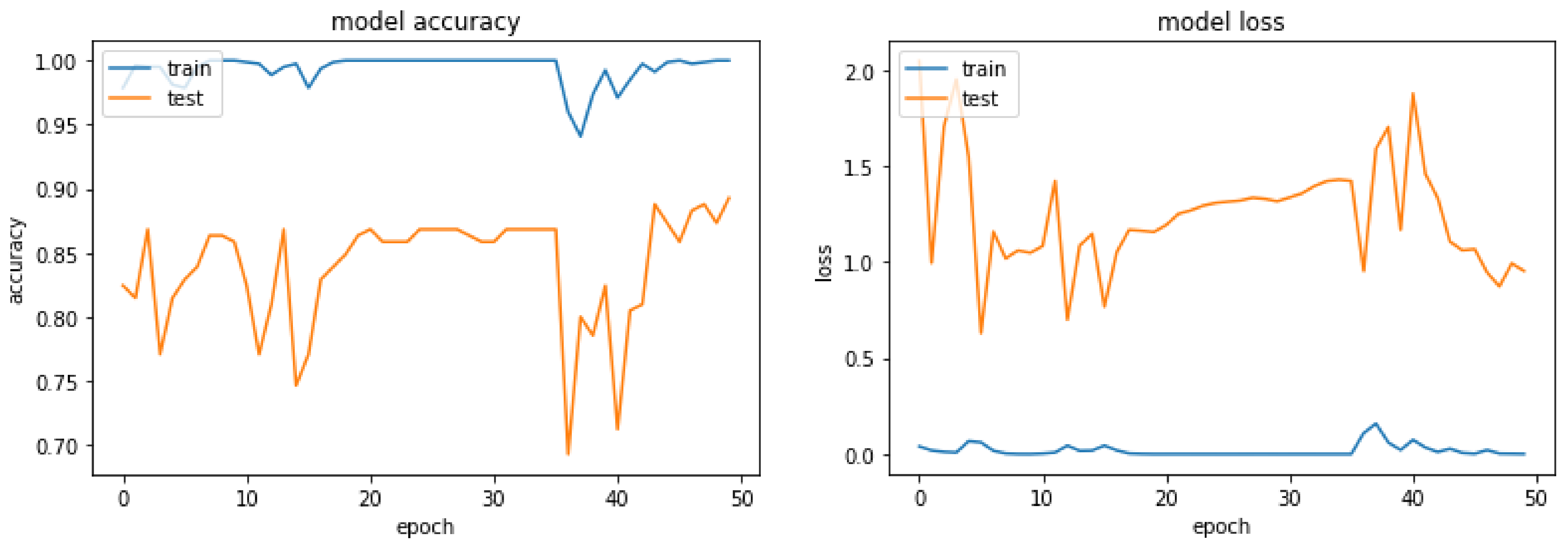
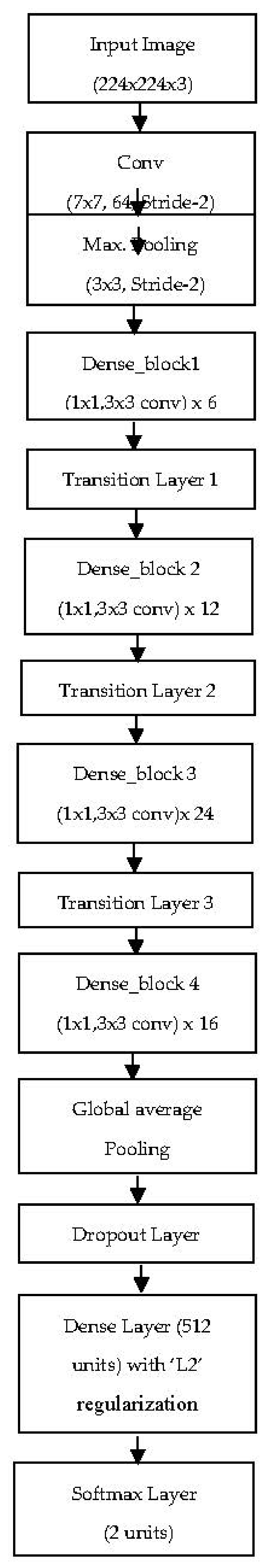
4.4. DenseNet121 Architecture

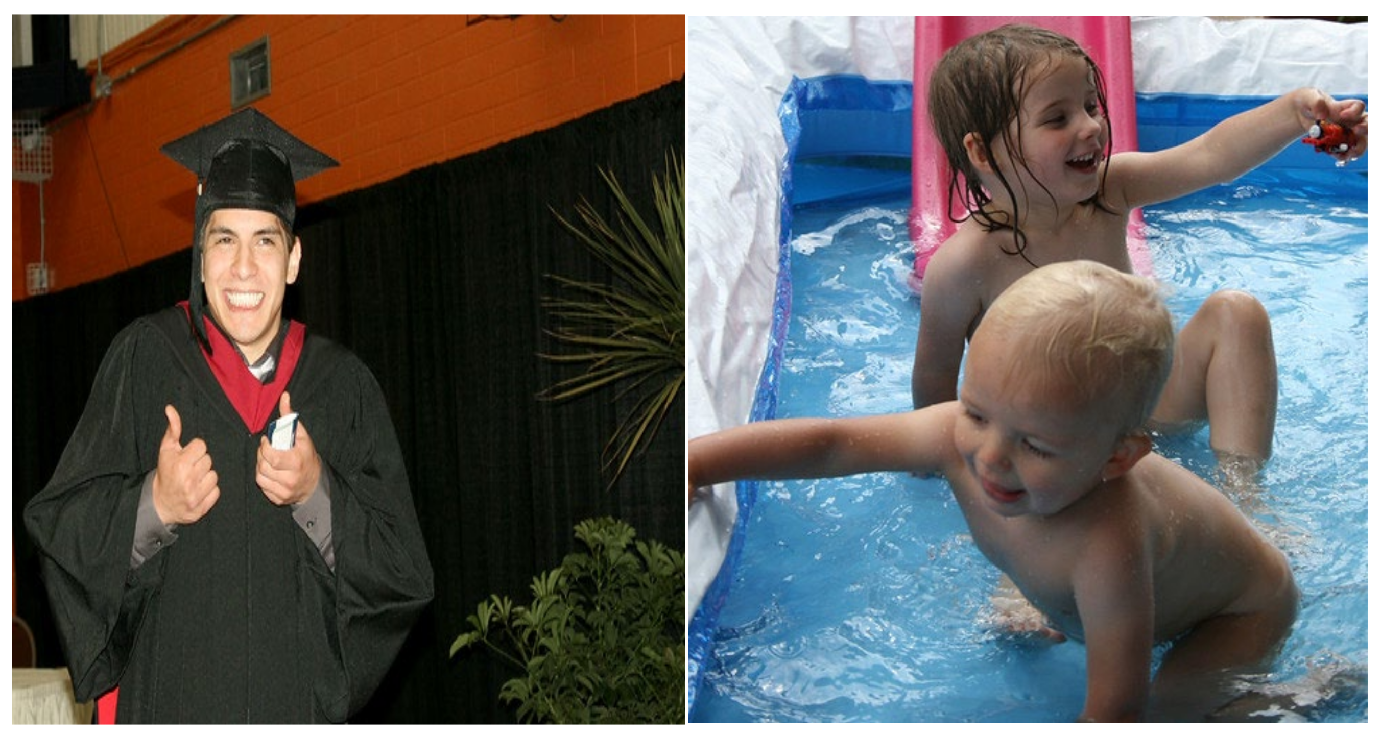
The DenseNet deep learning model was introduced to overcome the problem of vanishing gradients and to improve the system’s accuracy. It needs a lower number of parameters as well as a lower number of filters (12 filters/layer) compared to the ResNet model. It has a default input image size of 224 × 224 and its weights are trained on the ImageNet dataset. The DenseNet-121 model has 121 layers, 4 dense blocks, and transition layers in between them. Inside the dense blocks, there are certain numbers of convolutional layers that generate different feature maps. The transition layer’s job is to perform downsampling, which is done through a batch normalizing procedure. It aims to keep the feature maps generated by the max-pooling process as small as possible. The feature maps in each dense block in the DenseNet model have the same dimensions, and it concatenates the feature maps derived from prior layers, as shown by the following expression:

$$x_l=H_l\left(\left[x_0,x_1,\dots \dots x_{l-1}\right]\right)$$

(3)

where

$\left[x_0,x_1,\dots \dots x_{l-1}\right]$ represent the concatenated feature maps obtained from the earlier layers, that is, from the 0 to L1 layers.

$H_l$ represents the non-linear transformation function, with “l” indicating the layer number.

The DenseNet121 model has initial convolutional layers with output sizes of 112 × 112 × 64 and a max-pooling layer with output sizes of 56 × 56 × 64. This produced output is used as the first dense layer’s input. One important parameter is the growth rate “k”, which decides the dimensions of the channel at each layer. The different layers present in the basic DenseNet-121 architecture and the output size of the layers are presented in

Table 3. Layers in DenseNet121 architecture.

Name of the Layer	Size of the Output	DenseNet-121
Convolution	112 × 112	7 × 7 convolution with a stride of 2
Pooling	56 × 56	3 × 3 max pooling with a stride of 2
Dense Block 1	56 × 56	[1 × 1 and 3 × 3 conv] × 6
Transition Layer 1	28 × 28	[1 × 1] convolution with [2 × 2] average pooling layer
Dense Block 2	28 × 28	[1 × 1 and 3 × 3 conv] × 12
Transition Layer 2	14 × 14	[1 × 1 and 3 × 3 conv] × 6
Dense Block 3	14 × 14	[1 × 1 and 3 × 3 conv] × 24
Transition Layer 3	7 × 7	[1 × 1 and 3 × 3 conv] × 6
Dense Block 4	7 × 7	[1 × 1 and 3 × 3 conv] × 16
Classification	1 × 1	Global average pooling [7 × 7] with 1000 fully connected Softmax layers

below.

For positive and negative classification, we added additional layers, such as a global average pooling layer, a dropout layer, a dense layer (512 units) with an L2 regularizer, and a final dense layer (2 units). By freezing the layers of Block 1 and Block 2 of the network and unfreezing the remaining layers (Block 3 and Block 4) that were trained on the Crowdflower image sentiment dataset, we were able to fine-tune the network. The fine-tuned ResNet50 network architecture that we used in our research is illustrated in Figure 5 below.

5. Dataset

The pre-trained models (VGG-19, ResNet50V2, and DenseNet121) were evaluated on the image samples obtained from the Crowdflower image sentiment dataset (https://data.world/crowdflower/image-sentiment-polarity, accessed on 12 December 2021). The dataset has a large collection of image URLs with their sentiment polarity, and it is labeled by different annotators. It has different sentiment polarity classes, such as highly positive, positive, highly negative, negative, and neutral classes. We downloaded the images from this dataset containing the positive and negative classes only, totaling 1000 images. The numbers of positive and negative class image samples present in our dataset are shown in

Table 4. Input image database details.

Sentiment Class	Number of Images
Positive	642
Negative	358
Total	1000

below.

The following figures (Figure 6 and Figure 7) show some of the images belonging to the positive and negative sentiment classes that are available in the dataset.

6. Experimental Results and Discussion

Our work on image sentiment prediction was done with the help of Google Colaboratory (https://research.google.com/colaboratory/) (accessed on 12 December 2021), and the coding was done with the Python 3.5 language (https://devdocs.io/python~3.5/, accessed on 12 December 2021). We used a suitable Tesla GPU with a speed of 2.30 GHz, utilizing 16GB of RAM. The transfer learning model was built and run using the Keras Python library (https://keras.io/api/). The MatPlotLib library (https://matplotlib.org/) was used to plot the findings, and the SciKit-learn library (https://scikit-learn.org/stable/about.html, accessed on 12 December 2021) was used to create a confusion matrix.

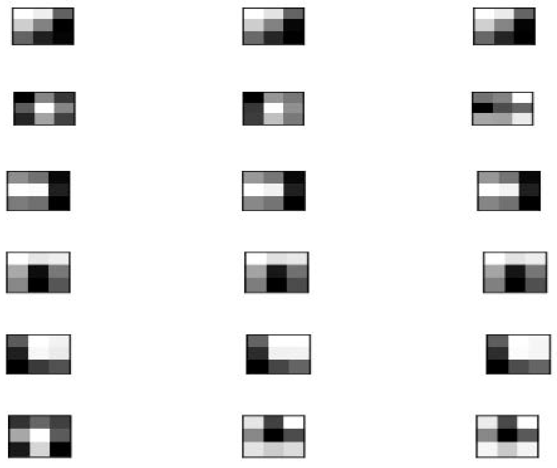
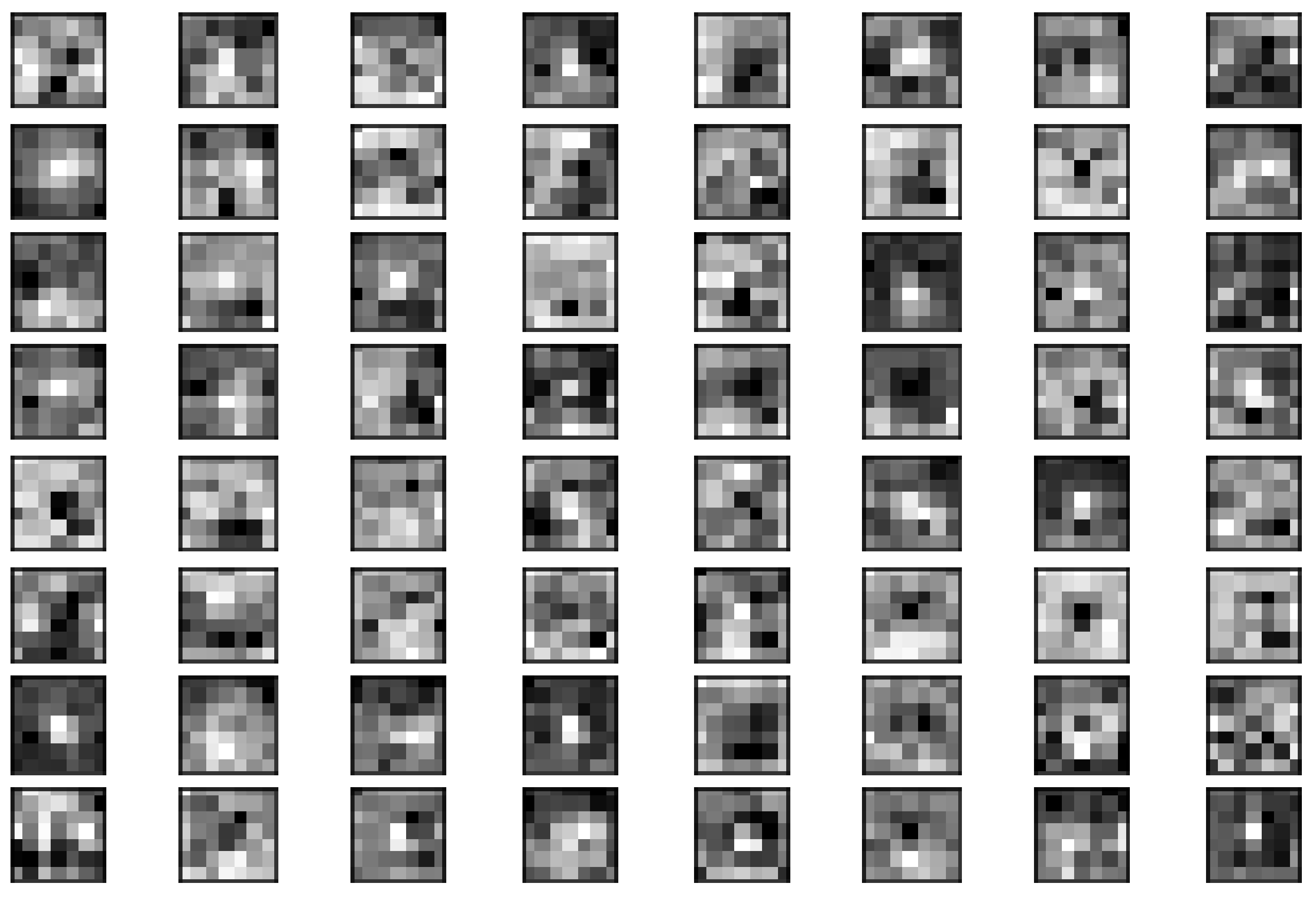
6.1. Visual Features from the First Convolutional Layer of VGG-19

The weight values of the filters in the first convolutional layer in Block 1 of the VGG-19 model were normalized to have values between 0 to 1. Figure 8 shows a sample input image from the dataset, and Figure 9 shows the first six filters out of the 64 filters in the first convolutional block. The Matplotlib library was used to plot each of the three filter channels, namely R, G, and B. Each row in the diagram represents a filter, whereas the column values indicate each channel (i.e., R, G, and B). The presence of small weights is shown as dark squares, and the large weights appear as light squares.

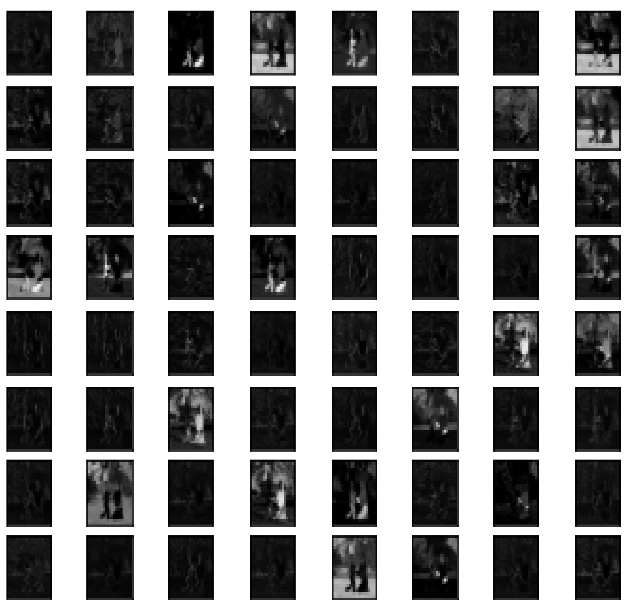
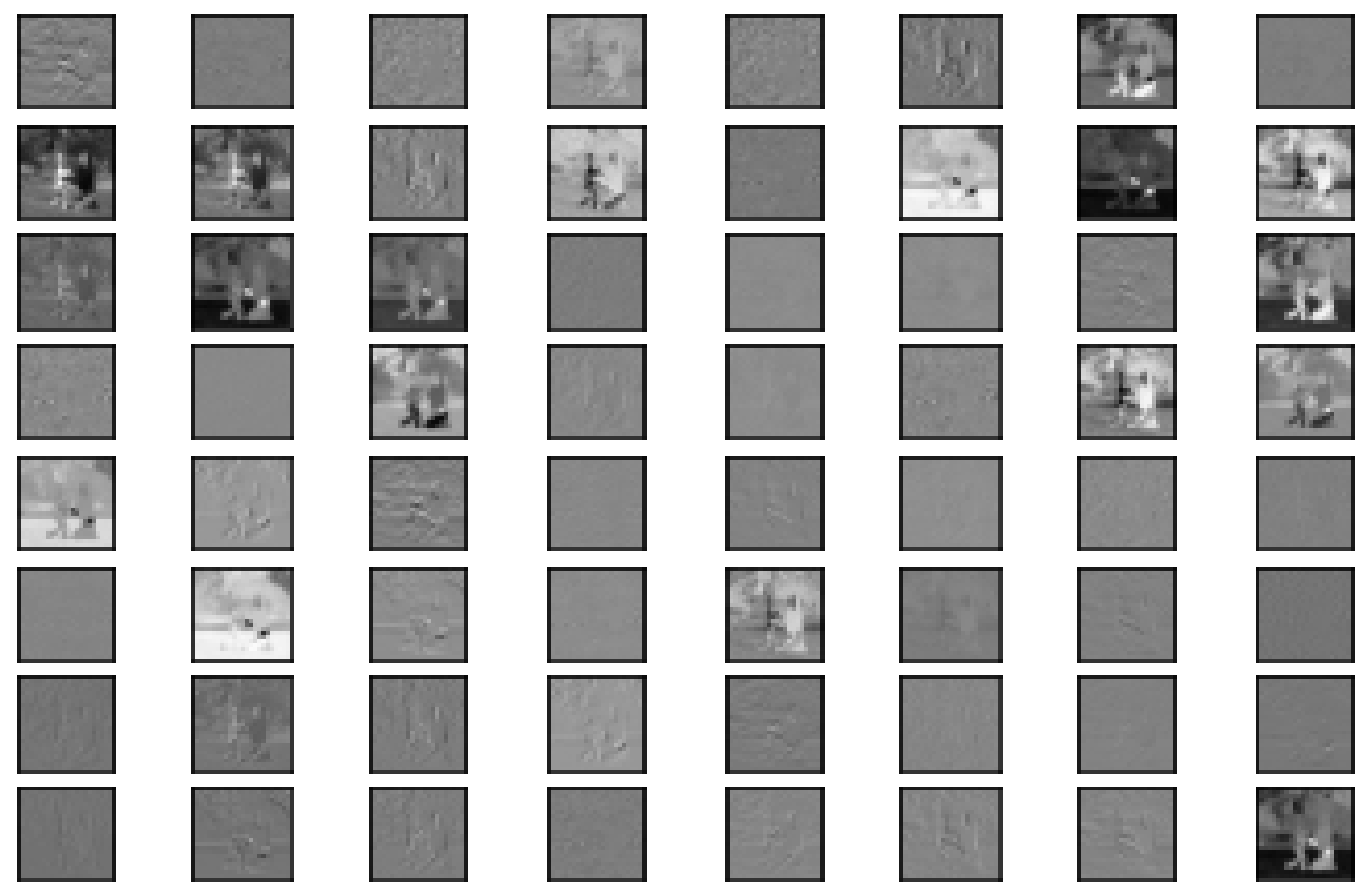
6.2. Feature Maps Extraction from VGG-19 Model

When we applied filters to the input image, we got feature maps, also known as activation maps. The feature maps near the input layer detected the small details in the image pixels, and the feature maps closer to the output found a higher level or more generalized features. We had five main convolutional blocks (Block 1, Block 2, Block 3, Block 4, and Block 5) in the VGG-19 model. The number of feature maps kept increasing, from 64 (Block 1) to 512 (Block 5) as we reached the last block. Figure 10 and Figure 11 show the feature maps extracted from the convolutional layers of the first (Block 1) and last blocks (Block 5) of the VGG-19 model.

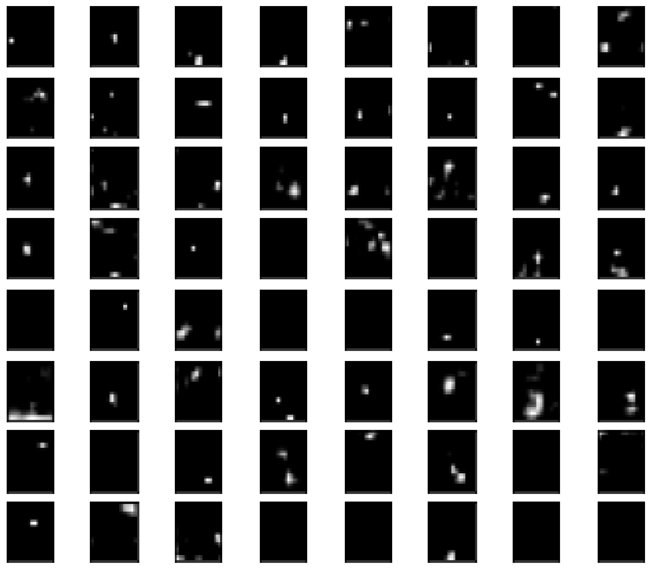
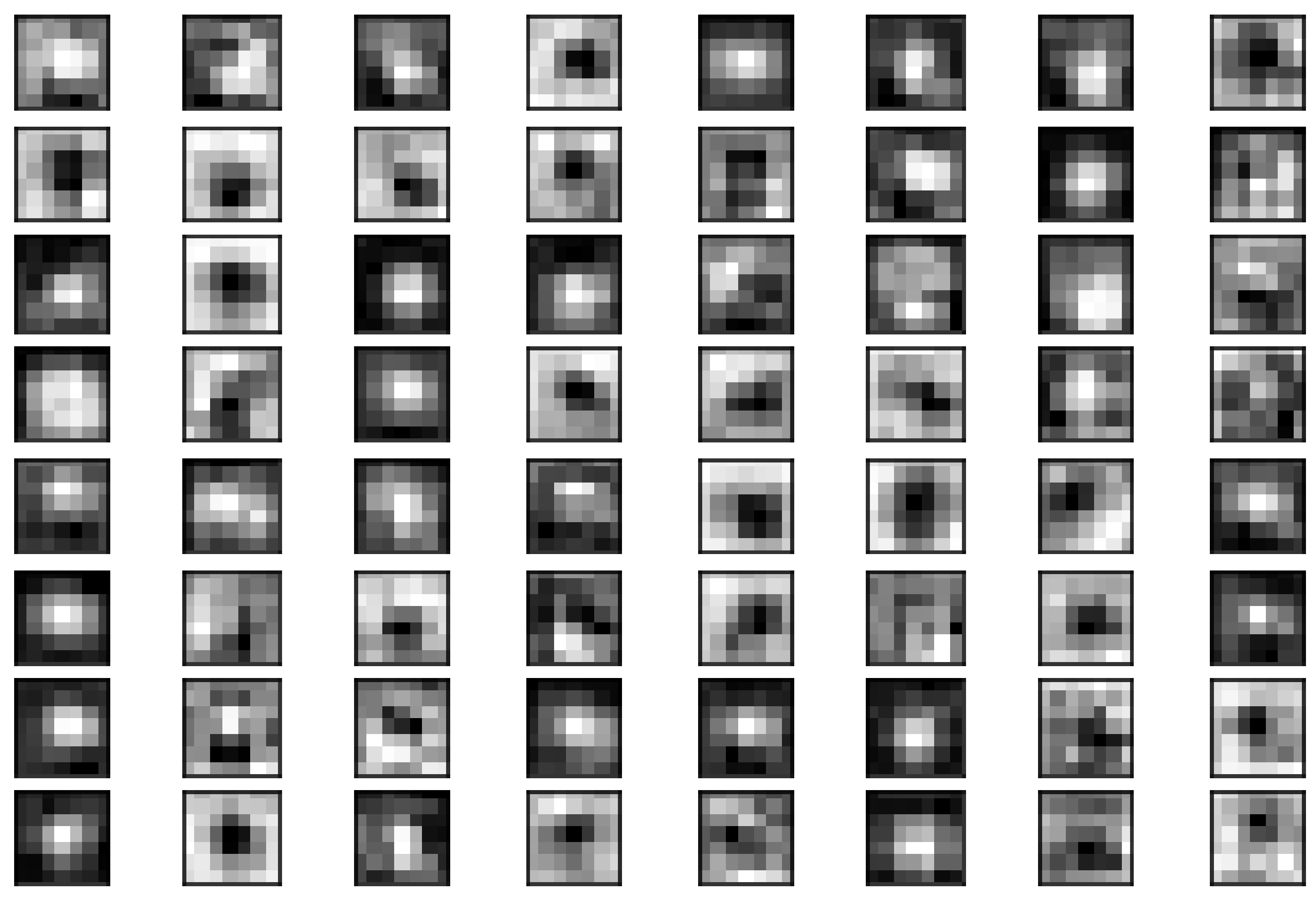
6.3. Feature Map Extraction from ResNet50V2 and DenseNet-121 Models

Figure 12 andFigure 13 show the feature maps extracted from the initial and final convolutional layers of the ResNet50V2 model.

Figure 14 and Figure 15 show the feature maps extracted from the initial and final convolutional layers of the DenseNet-121 model.

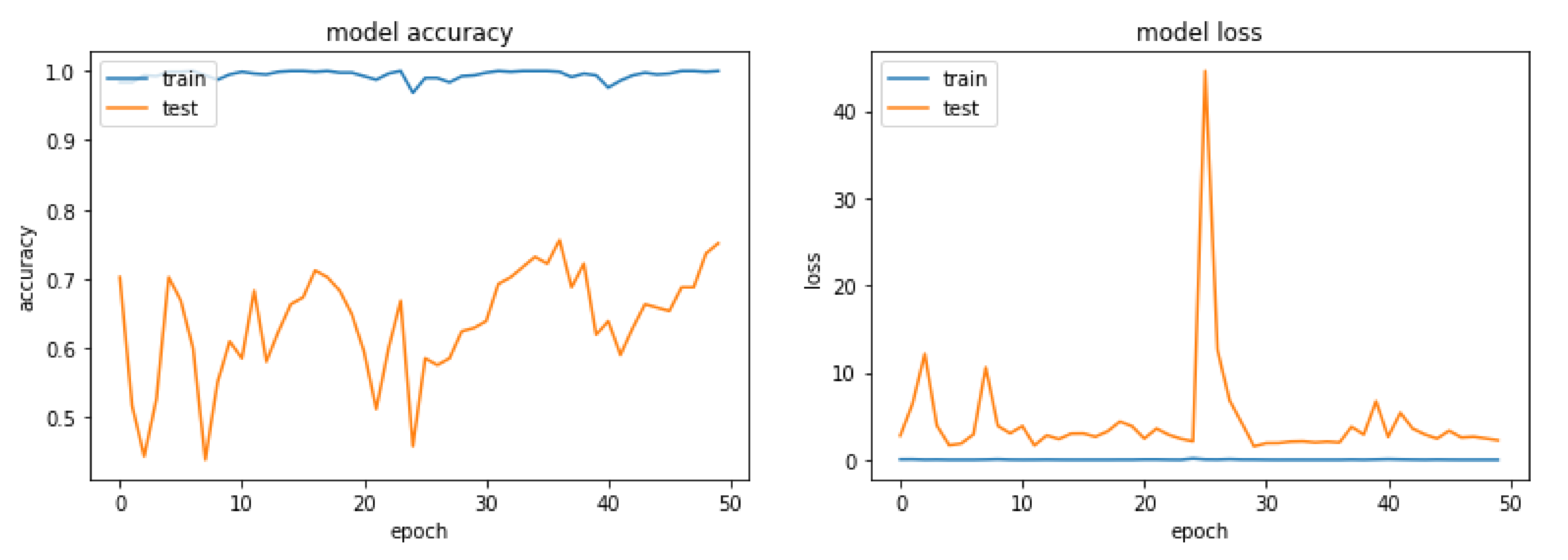
6.4. Result of Visual Sentiment Classification with the Fine-Tuned pre-Trained Models

The existing pre-trained models used in our work (VGG-19, Resnet50V2, and Densenet121) were imported from the Keras library and the ImageNet weights were used to train them. The flatten class available in the Keras library was used to convert the max-pooling layer output into a one-dimensional array of vectors. A long feature vector was created and the flatten layer’s output was normalized with a batch normalization layer. To reduce the problem of overfitting, a dropout layer was added and succeeded by a dense layer with 512 units. The network weights were penalized by adding the L2 regularization technique to avoid the effect of overfitting. The final dense layer (Softmax) had two units, corresponding to the number of sentiment classes (positive and negative).

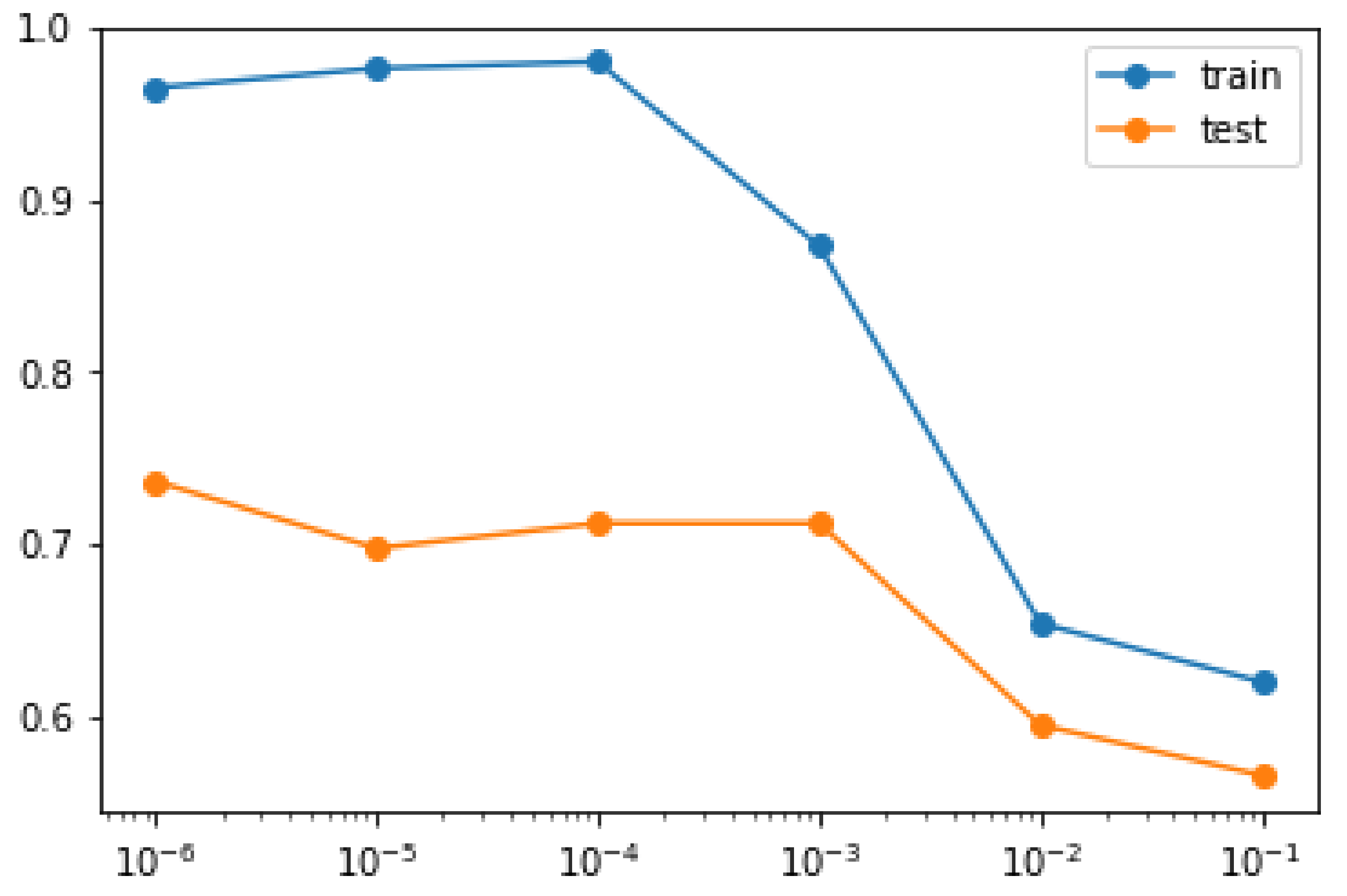
6.4.1. Weight Regularization

To reduce the overfitting of the models to the training data and to achieve performance improvement, we implemented the weight regularization (L2 regularization) concept. The weight regularizer was added to the dense layer with 512 units, which was placed just before the final dense layer with 2 units. It was implemented with the Keras weight regularization API, which helped add a penalty for the weights. The Keras API provided three different weight regularizations, namely the L1 regularization, which generates the sum of absolute weights, the sum of squared weights was generated by L2, and the combination of the sum of the absolute and squared weights was provided by the L1 and L2 regularizers. The L2 regularization technique was implemented with the help of the Keras library by summing up the squared weights of the model. We evaluated the model’s performance using various regularization parameter settings. We performed the grid search through different values of regularization parameter values of L2 regularization to find the value that gives higher accuracy with the model.

From Figure 16, we were able to conclude that the VGG-19 model achieved its highest accuracy of 75.21% when the value of the weight regularization parameter was 10⁻⁶. The training and testing accuracies of the model reached their lowest values when the value of the weight regularization parameter reached 10⁻¹.

Figure 16 andFigure 17 depict the classification accuracies achieved by choosing different values for the weight regularization parameter. From the plots, we were able to conclude that the DenseNet-121 model had its best value for testing accuracy, 89.26%, when the value of the weight regularization parameter was 10⁻². The Resnet50V2 model achieved its highest accuracy of 75.12% when the value of the weight regularization parameter was 10⁻⁶. The training and testing accuracies for both the models reached their lowest values when the value of the weight regularization parameter reached 10⁻¹.

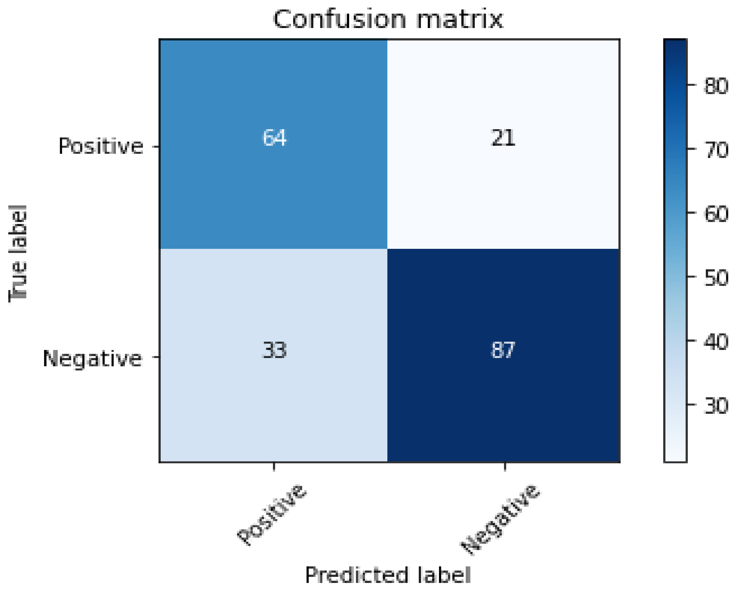
6.4.2. Generation of Confusion Matrix

The pre-trained models were compiled with a suitable optimizer (“Adam”). A loss function (“categorical cross-entropy”) was applied. The Adam optimizer can work perfectly even with large datasets and also has a learning rate that is adaptable. The training of the model was done with a set of images allocated for training with 50 epochs, and a batch size of 20 was maintained. After training, the model was evaluated using test samples. Figure 18 shows the confusion matrix generated after evaluating the testing samples with the fine-tuned VGG-19 model.

The confusion matrix generated by the DenseNet-121 and ResNet50V2 deep learning networks for image sentiment categorization is shown in Figure 19 below.

6.4.3. Generation of a Classification Report

The classification report of the different pre-trained models was generated using the SciKit-learn library, which gives the values of various performance metrics, such as accuracy, precision, recall, and F1 score, as shown in

Table 5. Performance metrics of the VGG-19 model for image sentiment classification.

VGG-19 Model
Sentiment Class	Precision	Recall	F1 Score
Positive	0.66	0.75	0.70
Negative	0.81	0.72	0.76
Accuracy	0.73

,

Table 6. Performance metrics of the DenseNet121 model for image sentiment classification.

DenseNet121 Model
Sentiment Class	Precision	Recall	F1 Score
Positive	0.86	0.88	0.87
Negative	0.92	0.90	0.91
Accuracy	0.89

and

Table 7. Performance metrics of the ResNet50V2 model for image sentiment prediction.

ResNet50V2 Model
Sentiment Class	Precision	Recall	F1 Score
Positive	0.74	0.62	0.68
Negative	0.76	0.84	0.80
Accuracy	0.75

.

$$\mathrm{Precision}=\frac{\mathrm{TP}}{\mathrm{TP}+\mathrm{FP}}$$

(4)

$$\mathrm{Recall}=\frac{\mathrm{TP}}{\mathrm{TP}+\mathrm{FN}}$$

(5)

$$\mathrm{F}1 \mathrm{Score}=2\ast \frac{\left(\mathrm{Precision} \ast \mathrm{Recall}\right)}{\left(\mathrm{Precision}+\mathrm{Recall}\right)}$$

(6)

$$\mathrm{Accuracy}=\frac{ \mathrm{TP}+\mathrm{TN}}{\mathrm{TP}+\mathrm{TN}+\mathrm{FP}+\mathrm{FN}}$$

(7)

TP—true positive, TN—true negative, FP—false positive, FN—false negative.

From the performance metrics, we can conclude that for the given input visual dataset, the fine-tuned DenseNet-121 model yielded the best accuracy (0.89) compared to the other two (VGG-19 and ResNet50V2) transfer learning models.

6.4.4. Performance Comparison of the Different Transfer Learning Models

The following plots (Figure 20, Figure 21 and Figure 22) help us to have a clear visualization of the model loss and accuracy generated by the different pre-trained models. It is easy to make out the comparative analysis of these models from the plots shown below.

The above plots show the model accuracy and model loss over the epoch for 50 epochs. It is indicated that the fine-tuned DesneNet121 model had the highest testing accuracy. The maximum model loss was at the beginning of the epoch and continued to decrease as it went beyond 4 epochs, settling to a lower value as it neared 50 epochs. When we evaluated the proposed and other transfer learning models on the collected dataset, we noted that the performance increased when there was a much deeper architecture, such as DenseNet121, in our dataset.

7. Comparison of Our Work to Existing Image Sentiment Analysis Research

Many previous studies have used several advanced machine learning models to do sentiment classification on images. We compared our findings to the other recent research works related to image sentiment analysis. Although the comparison is not really equitable since the other papers used different datasets, it does provide insight into the characteristics behind it and the classification approach used with their outcomes.

Table 8. Comparison of existing works with our image sentiment analysis model.

S. No.	Author Name	Technique Used and Results	Merits	Limitations
1	Jing Zhang et al. [44]	Convolutional neural networks (CNN) was employed. On social media, researchers achieved a prediction accuracy of 68.02%.	Using several fusion algorithms, good performance on image sentiment categorization was attained.	A shallow structure may not be adequate for learning high-level semantic information.
2	Quanzeng You and Jiebo Luo [45]	Convolutional neural networks (CNN) with fine-tuned parameters achieved an accuracy of 58.3% for sentiment prediction on social media images.	The introduction of deep visual characteristics improved sentiment prediction task performance.	The performance of using deep visual features is not consistent across the sentiment categories.
3	Jindal, S. and Singh, S. [46]	A CNN with domain-specific tuning was used. Sentiment prediction on social media data yielded an accuracy of 53.5%.	Domain-specific tuning helps in better sentiment prediction.	The overfitting needs to be reduced and some challenges must be overcome to obtain enhanced performance.
4	Fengjiao, W. and Aono M. [47]	CNN was used in conjunction with Bag-of-Visual-Words (BOVW) features. On the Twitter images dataset, researchers achieved an accuracy of 72.2% for sentiment prediction.	The performance of sentiment prediction is improved by combining hand-crafted features with CNN features.	To determine the model’s efficiency, a substantial training dataset must be used.
5	Siqian Chen and Jie Yang [48]	To learn the visual features, the Alexnet model was employed. Sentiment prediction from social media images achieved an accuracy score of 48.08%.	By incorporating label information into the collective matrix factorization (CMF) technique, prediction accuracy is improved.	To achieve better outcomes, more constraints must be applied to the CMF technique, and the Alexnet model must be fine-tuned.
6	Papiya Das et al. [49]	SVM classification layer was used on deep CNN architecture. On various visual datasets, the accuracies were 65.89% and 68.67%.	The application of attention models aid in mapping the local regions of an image, resulting in better sentiment prediction.	To improve sentiment prediction performance, a strong visual classifier with robust feature identification methodologies is required.
7	Yun Liang et al. [50]	The cross-domain semi-supervised deep metric earning (CDSS-DML) method was used. For social media image sentiment prediction, it obtained an overall accuracy score of 0.44.	The model is trained with unlabeled data based on the teacher–student paradigm, overcoming the limits imposed by the scarcity of well-labeled data.	It is necessary to investigate the concept of fine-tuning the model in order to improve its effectiveness.
8	Chuang Lin et al. [51]	The multisource sentiment generative adversarial network (MSGAN) method was used and, for visual sentiment prediction, an accuracy of 70.63% was obtained.	Very efficient at dealing with data from numerous source domains.	Methods for improving the inherent flaws of the GAN network must be investigated further.
9	Dongyu She et al. [52]	Weakly supervised coupled convolutional network (WSCCN) was used. On several datasets of images, the highest accuracy of 0.86% was obtained for sentiment prediction.	Reduces annotation burden by picking useful soft proposals from weak annotations automatically.	To improve the findings, pre-processing strategies must be investigated.
10	The proposed approach (fine-tuned pre-trained models) Ganesh Chandrasekaran et al.	Various fine-tuned pre-trained models, namely the VGG-19, ResNet50V2, and DenseNet-121, were used. With an accuracy of 0.89, the DenseNet-121 model fared better.	By using dropout and regularization layers with fine-tuning, it addresses the limitations of overfitting caused by the lack of training data.	To increase sentiment prediction results, more samples must be added to the training set, and an extra modality (text or audio) can be used.

, below, compares various existing studies with our strategy for image sentiment analysis.

8. Conclusions and Future Work

In our research work, we compared the performance of the three pre-trained models (VGG-19, DenseNet121, and ResNet50V2) to predict the sentiments from images. We fine-tuned the models to improve their performance by unfreezing a part of the model and freezing the initial layers. Some additional layers, such as the dropout, batch normalization, and weight regularization layers, were used to reduce the effect of overfitting. By adding these layers, the model could perform better on our dataset for analyzing sentiments. After comparing the models based on their performance metrics, we were able to deduce that the DenseNet121 model performed well compared to the other two models (VGG-19 and ResNet50V2). The best accuracy (0.89) was obtained with the DenseNet121 model for the image sentiment analysis on our dataset. Our future work will focus on increasing the number of images used to train the model and combining multiple modalities to improve the model’s performance.

References

1. Karray, F.; Alemzadeh, M.; Abou Saleh, J.; Nours Arab, M. Human-Computer Interaction: Overview on State of the Art. Int. J. Smart Sens. Intell. Syst. 2008, 1, 137–159. [Google Scholar] [CrossRef] [Green Version]
2. Auxier, B.; Anderson, M. Social media use in 2021. Pew Res. Cent. 2021. [Google Scholar]
3. Sivarajah, U.; Kamal, M.M.; Irani, Z.; Weerakkody, V. Critical analysis of Big Data challenges and analytical methods. J. Bus. Res. 2017, 70, 263–286. [Google Scholar] [CrossRef] [Green Version]
4. Bansal, B.; Srivastava, S. On predicting elections with hybrid topic based sentiment analysis of tweets. Procedia Comput. Sci. 2018, 135, 346–353. [Google Scholar] [CrossRef]
5. El Alaoui, I.; Gahi, Y.; Messoussi, R.; Chaabi, Y.; Todoskoff, A.; Kobi, A. A novel adaptable approach for sentiment analysis on big social data. J. Big Data 2018, 5, 12. [Google Scholar] [CrossRef]
6. Drus, Z.; Khalid, H. Sentiment Analysis in Social Media and Its Application: Systematic Literature Review. Procedia Comput. Sci. 2019, 161, 707–714. [Google Scholar] [CrossRef]
7. Zhao, H.; Liu, Z.; Yao, X.; Yang, Q. A machine learning-based sentiment analysis of online product reviews with a novel term weighting and feature selection approach. Inf. Processing Manag. 2021, 58, 102656. [Google Scholar] [CrossRef]
8. Dashtipour, K.; Gogate, M.; Adeel, A.; Larijani, H.; Hussain, A. Sentiment Analysis of Persian Movie Reviews Using Deep Learning. Entropy 2021, 23, 596. [Google Scholar] [CrossRef]
9. Farisi, A.A.; Sibaroni, Y.; Faraby, S.A. Sentiment analysis on hotel reviews using Multinomial Naïve Bayes classifier. J. Phys. Conf. Ser. 2019, 1192, 012024. [Google Scholar] [CrossRef]
10. Melton, C.A.; Olusanya, O.A.; Ammar, N.; Shaban-Nejad, A. Public sentiment analysis and topic modeling regarding COVID-19 vaccines on the Reddit social media platform: A call to action for strengthening vaccine confidence. J. Infect. Public Health 2021, 14, S1876034121002288. [Google Scholar] [CrossRef]
11. Mishra, N.; Jha, C.K. Classification of Opinion Mining Techniques. Int. J. Comput. Appl. 2012, 56, 1–6. [Google Scholar] [CrossRef]
12. Kim, M.; Lee, S.M.; Choi, S.; Kim, S.Y. Impact of visual information on online consumer review behavior: Evidence from a hotel booking website. J. Retail. Consum. Serv. 2021, 60, 102494. [Google Scholar] [CrossRef]
13. Xiao, Z.; Wang, L.; Du, J.Y. Improving the Performance of Sentiment Classification on Imbalanced Datasets With Transfer Learning. IEEE Access 2019, 7, 28281–28290. [Google Scholar] [CrossRef]
14. Praveen Gujjar, J.; Prasanna Kumar, H.R.; Chiplunkar, N.N. Image Classification and Prediction using Transfer Learning in Colab Notebook. Glob. Transit. Proc. 2021, 2, S2666285X21000960. [Google Scholar] [CrossRef]
15. Zhang, Q.; Yang, Q.; Zhang, X.; Bao, Q.; Su, J.; Liu, X. Waste image classification based on transfer learning and convolutional neural network. Waste Manag. 2021, 135, 150–157. [Google Scholar] [CrossRef]
16. Dilshad, S.; Singh, N.; Atif, M.; Hanif, A.; Yaqub, N.; Farooq, W.A.; Ahmad, H.; Chu, Y.; Masood, M.T. Automated image classification of chest X-rays of COVID-19 using deep transfer learning. Results Phys. 2021, 28, 104529. [Google Scholar] [CrossRef]
17. Siersdorfer, S.; Minack, E.; Deng, F.; Hare, J. Analyzing and predicting sentiment of images on the social web. In Proceedings of the International Conference on Multimedia MM ’10, Firenze, Italy, 25–29 October 2010; pp. 715–718. [Google Scholar] [CrossRef] [Green Version]
18. Rao, T.; Xu, M.; Liu, H.; Wang, J.; Burnett, I. Multi-scale blocks based image emotion classification using multiple instance learning. In Proceedings of the 2016 IEEE International Conference on Image Processing (ICIP), Phoenix, AZ, USA, 25–28 September 2016; pp. 634–638. [Google Scholar] [CrossRef]
19. Datta, R.; Joshi, D.; Li, J.; Wang, J.Z. Studying Aesthetics in Photographic Images Using a Computational Approach. In Computer Vision—ECCV 2006; Leonardis, A., Bischof, H., Pinz, A., Eds.; Springer: Berlin/Heidelberg, Germany, 2006; Volume 3953, pp. 288–301. [Google Scholar] [CrossRef]
20. Marchesotti, L.; Perronnin, F.; Larlus, D.; Csurka, G. Assessing the aesthetic quality of photographs using generic image descriptors. In Proceedings of the 2011 International Conference on Computer Vision, Barcelona, Spain, 6–13 November 2011; pp. 1784–1791. [Google Scholar] [CrossRef]
21. Borth, D.; Chen, T.; Ji, R.; Chang, S.-F. SentiBank: Large-scale ontology and classifiers for detecting sentiment and emotions in visual content. In Proceedings of the 21st ACM International Conference on Multimedia—M ’13, Barcelona, Spain, 21–25 October 2013; pp. 459–460. [Google Scholar] [CrossRef]
22. Yuan, J.; Mcdonough, S.; You, Q.; Luo, J. Sentribute: Image sentiment analysis from a mid-level perspective. In Proceedings of the Second International Workshop on Issues of Sentiment Discovery and Opinion Mining—WISDOM ’13, Chicago, IL, USA, 11 August 2013; pp. 1–8. [Google Scholar] [CrossRef]
23. Zhao, Z.; Zhu, H.; Xue, Z.; Liu, Z.; Tian, J.; Chua, M.C.H.; Liu, M. An image-text consistency driven multimodal sentiment analysis approach for social media. Inf. Processing Manag. 2019, 56, 102097. [Google Scholar] [CrossRef]
24. Fernandez, D.; Woodward, A.; Campos, V.; Giro-i-Nieto, X.; Jou, B.; Chang, S.-F. More cat than cute? Interpretable Prediction of Adjective-Noun Pairs. In Proceedings of the Workshop on Multimodal Understanding of Social, Affective and Subjective Attributes, Mountain View, CA, USA, 27 October 2017; pp. 61–69. [Google Scholar] [CrossRef] [Green Version]
25. Yang, J.; She, D.; Sun, M.; Cheng, M.-M.; Rosin, P.L.; Wang, L. Visual Sentiment Prediction Based on Automatic Discovery of Affective Regions. IEEE Trans. Multimed. 2018, 20, 2513–2525. [Google Scholar] [CrossRef] [Green Version]
26. Wang, J.; Fu, J.; Xu, Y.; Mei, T. Beyond Object Recognition: Visual Sentiment Analysis with Deep Coupled Adjective and Noun Neural Networks. In Proceedings of the Twenty-Fifth International Joint Conference on Artificial Intelligence (IJCAI-16), New York, NY, USA, 9–15 July 2016; pp. 3484–3490. [Google Scholar]
27. Song, K.; Yao, T.; Ling, Q.; Mei, T. Boosting image sentiment analysis with visual attention. Neurocomputing 2018, 312, 218–228. [Google Scholar] [CrossRef]
28. Ortis, A.; Farinella, G.M.; Torrisi, G.; Battiato, S. Visual Sentiment Analysis Based on on Objective Text Description of Images. In Proceedings of the 2018 International Conference on Content-Based Multimedia Indexing (CBMI), La Rochelle, France, 4–6 September 2018; pp. 1–6. [Google Scholar] [CrossRef]
29. Xu, J.; Huang, F.; Zhang, X.; Wang, S.; Li, C.; Li, Z.; He, Y. Sentiment analysis of social images via hierarchical deep fusion of content and links. Appl. Soft Comput. 2019, 80, 387–399. [Google Scholar] [CrossRef]
30. Huang, F.; Zhang, X.; Zhao, Z.; Xu, J.; Li, Z. Image-text sentiment analysis via deep multimodal attentive fusion. Knowl. Based Syst. 2019, 167, 26–37. [Google Scholar] [CrossRef]
31. Chen, T.; Borth, D.; Darrell, T.; Chang, S.-F. DeepSentiBank: Visual Sentiment Concept Classification with Deep Convolutional Neural Networks. ArXiv 2014, arXiv:1410.8586. [Google Scholar]
32. Campos, V.; Jou, B.; Giró-i-Nieto, X. From Pixels to Sentiment: Fine-tuning CNNs for Visual Sentiment Prediction. Image Vis. Comput. 2016, 65, 15–22. [Google Scholar] [CrossRef] [Green Version]
33. Machajdik, J.; Hanbury, A. Affective image classification using features inspired by psychology and art theory. In Proceedings of the International Conference on Multimedia—MM ’10, Firenze, Italy, 25–29 October 2010; pp. 83–92. [Google Scholar] [CrossRef]
34. Katsurai, M.; Satoh, S. Image sentiment analysis using latent correlations among visual, textual, and sentiment views. In Proceedings of the 2016 IEEE International Conference on Acoustics, Speech and Signal Processing (ICASSP), Shanghai, China, 20–25 March 2016; pp. 2837–2841. [Google Scholar] [CrossRef]
35. Yilin, W.; Suhang, W.; Jiliang, T.; Huan, L.; Baoxin, L. Unsupervised Sentiment Analysis for Social Media Images. In Proceedings of the Twenty-Fourth International Joint Conference on Artificial Intelligence (IJCAI 2015), Buenos Aires, Argentina, 25–31 July 2015; pp. 2378–2379. [Google Scholar]
36. Zhang, S.; Zhang, X.; Chan, J.; Rosso, P. Irony detection via sentiment-based transfer learning. Inf. Processing Manag. 2019, 56, 1633–1644. [Google Scholar] [CrossRef]
37. Smetanin, S.; Komarov, M. Deep transfer learning baselines for sentiment analysis in Russian. Inf. Processing Manag. 2021, 58, 102484. [Google Scholar] [CrossRef]
38. Kanclerz, K.; Miłkowski, P.; Kocoń, J. Cross-lingual deep neural transfer learning in sentiment analysis. Procedia Comput. Sci. 2020, 176, 128–137. [Google Scholar] [CrossRef]
39. Xiao, M.; Wu, Y.; Zuo, G.; Fan, S.; Yu, H.; Shaikh, Z.A.; Wen, Z. Addressing Overfitting Problem in Deep Learning-Based Solutions for Next Generation Data-Driven Networks. Wirel. Commun. Mob. Comput. 2021, 2021, 1–10. [Google Scholar] [CrossRef]
40. Zhao, W. Research on the deep learning of the small sample data based on transfer learning. AIP Conf. Proc. 2017, 1864, 020018. [Google Scholar] [CrossRef] [Green Version]
41. Szegedy, C.; Ioffe, S.; Vanhoucke, V.; Alemi, A. Inception-v4, Inception-ResNet and the Impact of Residual Connections on Learning. ArXiv 2016, arXiv:1602.07261. [Google Scholar]
42. Huang, G.; Liu, Z.; van der Maaten, L.; Weinberger, K.Q. Densely Connected Convolutional Networks. ArXiv 2018, arXiv:1608.06993. [Google Scholar]
43. Deng, J.; Dong, W.; Socher, R.; Ki, L.; Li, K.; Fei-Fei, K. ImageNet: A large-scale hierarchical image database. In Proceedings of the IEEE Conference on Computer Vision and Pattern Recognition, Miami Beach, FL, USA, 20–25 June 2009. [Google Scholar]
44. Zhang, J.; Chen, M.; Sun, H.; Li, D.; Wang, Z. Object semantics sentiment correlation analysis enhanced image sentiment classification. Knowl. Based Syst. 2020, 191, 105245. [Google Scholar] [CrossRef]
45. You, Q.; Luo, J.; Jin, H.; Yang, J. Building a Large Scale Dataset for Image Emotion Recognition: The Fine Print and The Benchmark. ArXiv 2016, arXiv:1605.02677. [Google Scholar]
46. Jindal, S.; Singh, S. Image sentiment analysis using deep convolutional neural networks with domain specific fine tuning. In Proceedings of the 2015 International Conference on Information Processing (ICIP), Pune, India, 16–19 December 2015; pp. 447–451. [Google Scholar] [CrossRef]
47. Fengjiao, W.; Aono, M. Visual Sentiment Prediction by Merging Hand-Craft and CNN Features. In Proceedings of the 2018 5th International Conference on Advanced Informatics: Concept Theory and Applications (ICAICTA), Krabi, Thailand, 14–17 August 2018; pp. 66–71. [Google Scholar] [CrossRef]
48. Chen, S.; Yang, J.; Feng, J.; Gu, Y. Image sentiment analysis using supervised collective matrix factorization. In Proceedings of the 2017 12th IEEE Conference on Industrial Electronics and Applications (ICIEA), Siem Reap, Cambodia, 18–20 June 2017; pp. 1033–1038. [Google Scholar] [CrossRef]
49. Das, P.; Ghosh, A.; Majumdar, R. Determining Attention Mechanism for Visual Sentiment Analysis of an Image using SVM Classifier in Deep learning based Architecture. In Proceedings of the 2020 8th International Conference on Reliability, Infocom Technologies and Optimization (Trends and Future Directions) (ICRITO), Noida, India, 4–5 June 2020; pp. 339–343. [Google Scholar] [CrossRef]
50. Liang, Y.; Maeda, K.; Ogawa, T.; Haseyama, M. Cross-Domain Semi-Supervised Deep Metric Learning for Image Sentiment Analysis. In Proceedings of the ICASSP 2021–2021 IEEE International Conference on Acoustics, Speech and Signal Processing (ICASSP), Toronto, ON, Canada, 6–11 June 2021; pp. 4150–4154. [Google Scholar] [CrossRef]
51. Lin, C.; Zhao, S.; Meng, L.; Chua, T.-S. Multi-source Domain Adaptation for Visual Sentiment Classification. ArXiv 2020, arXiv:2001.03886. [Google Scholar]
52. She, D.; Yang, J.; Cheng, M.-M.; Lai, Y.-K.; Rosin, P.L.; Wang, L. WSCNet: Weakly Supervised Coupled Networks for Visual Sentiment Classification and Detection. IEEE Trans. Multimed. 2019, 22, 1358–1371. [Google Scholar] [CrossRef] [Green Version]
Figure 1. Flow diagram of the image sentiment prediction model.
Applsci 12 01030 g001
Figure 2. The VGG-19 architecture.
Applsci 12 01030 g002
Figure 4. Architecture of fine-tuned ResNet50V2 network.
Applsci 12 01030 g004
Figure 5. Architecture of fine-tuned DenseNet121 network.
Applsci 12 01030 g005
Figure 6. Example of positive sentiment images from the dataset.
Applsci 12 01030 g006
Figure 7. Example of negative sentiment images from the dataset.
Applsci 12 01030 g007
Figure 8. A sample input image from the dataset.
Applsci 12 01030 g008
Figure 9. Image features of the first 6 filters in the first convolutional layer of the VGG-19 model.
Applsci 12 01030 g009
Figure 10. Image features of first 6 filters in the first convolutional layer of the VGG-19 model.
Applsci 12 01030 g010
Figure 11. Feature map from Block 5 of the VGG-19 model.
Applsci 12 01030 g011
Figure 12. Feature map from initial convolutional layer (Conv 1) of the ResNet50V2 model.
Applsci 12 01030 g012
Figure 13. Feature map from last convolutional layer (Conv 4) of the ResNet50V2 model.
Applsci 12 01030 g013
Figure 14. Feature map from Dense_Block1 of the DenseNet-121 model.
Applsci 12 01030 g014
Figure 15. Feature map from Dense_Block4 of the DenseNet-121 model.
Applsci 12 01030 g015
Figure 16. Accuracy plot of the grid search of regularization parameter (VGG-19 model).
Applsci 12 01030 g016
Figure 17. Accuracy plot of the grid search of regularization parameter (DenseNet-121 and Resnet50V2 models).
Applsci 12 01030 g017
Figure 18. Confusion matrix generated by the VGG-19 model.
Applsci 12 01030 g018
Figure 19. Confusion matrix generated by the DenseNet121 and ResNet50V2 models.
Applsci 12 01030 g019
Figure 20. Model accuracy and model loss plots of the VGG-19 model for image sentiment prediction.
Applsci 12 01030 g020
Figure 21. Model accuracy and model loss plots of the DenseNet121 model for image sentiment prediction.
Applsci 12 01030 g021
Figure 22. Model accuracy and model loss plots of the ResNet50V2 model for image sentiment prediction.
Applsci 12 01030 g022