Skeleton Motion Recognition Based on Multi-Scale Deep Spatio-Temporal Features

Abstract

In the task of human motion recognition, the overall action span is changeable, and there may be an inclusion relationship between action semantics. This paper proposes a novel multi-scale time sampling module and a deep spatiotemporal feature extraction module, which strengthens the receptive field of the feature map and strengthens the extraction of spatiotemporal-related feature information via the network. We study and compare the performance of three existing multi-channel fusion methods to improve the recognition accuracy of the network on the open skeleton recognition dataset. In this paper, several groups of comparative experiments are carried out on two public datasets. The experimental results show that compared with the classical 2s-AGCN algorithm, the accuracy of the algorithm proposed in this paper shows an improvement of 1% on the Kinetics dataset and 0.4% and 1% on the two evaluating indicators of the NTU-RGB+D dataset, respectively.

1. Introduction

With the rapid development of deep learning technology and artificial intelligence algorithms, human motion recognition, especially motion recognition based on human bones, has attracted extensive attention from scholars all over the world [1,2,3]. Motion recognition plays a very important role in intelligent monitoring systems, human–computer interaction systems, intelligent robots, virtual reality technology, automatic driving, motion correction, and so on. For example, it is involved in analyzing an athletes’ sports posture to improve the athlete’s sports performance and in automatic driving, by judging human movements and predicting their action intention. Traditional motion recognition methods mainly used the approach of manually designing features to extract information on features, train the classifier, and output the prediction results. This recognition method not only consumes a lot of resources but also can not meet the requirements of speed and accuracy [4,5].

In recent years, with the development of artificial intelligence technology and computer hardware, action recognition algorithms based on deep learning have been widely used because of their strong adaptability and high recognition efficiency. Action recognition based on deep learning can be divided into two categories. The first is based on the use of traditional CNN, RNN, or LSTM networks, such as two stream [6,7], C3D [8], and LSTM [9] methods. These use end-to-end learning to effectively reduce the amounts of parameters and greatly improve the recognition accuracy. Inspired by the process of human vision and the understanding of video information, Karens et al. [6] designed a dual-stream network. The two streams extracted time information and spatial information, respectively, and finally fused the two models. Du T et al. [8] found that a 3D convolution network is better than a 2D convolution network in learning spatiotemporal features, and proved through experiments that the use of a 3 × 3 × 3 convolution kernel for 3D convolution was the best. Jeff D et al. [9] proposed the long short-term memory (LSTM) network. Later generations used this network with action recognition tasks to learn effective features and model the dynamic process in the time domain to realize end-to-end action recognition and detection. The second category of the action recognition methods is those based on the human skeleton, which show better robustness to illumination changes and environmental changes. In recent years, this area has attracted extensive attention. The method uses a human posture detection algorithm and a high-precision depth camera to obtain the characteristics of a human skeleton, forms a graph through natural human connections, and gives a time series of human joint positions. With the rapid development of graph convolutional neural networks (GCNs), a large number of graph convolution-based network models have been applied to skeleton-based action recognition tasks. Yan et al. [10] first applied a graph convolution network to human skeleton action recognition, establishing the spatial graph of natural human connections, added time edges between corresponding joints in continuous time frames, and proposed a spatiotemporal graph convolution neural network. Kalpit T et al. [11] defined a partition of a skeleton graph. In this partition, spatiotemporal convolution was formalized using a location-based GCN for the task of action recognition; Shi et al. [12] proposed a two-stream adaptive graph convolution model to adaptively learn the graph topology of different GCN layers and skeleton samples, which was better adapted to the recognition task and GCN hierarchy, and further improved the recognition performance. At present, there are still some problems in the action recognition model based on graph convolution neural networks. (1) Different action durations are different and changeable. The current model still uses the characteristics of a single scale [13], and the information obtained on the same scale is very limited, which is not conducive to the improvement of the accuracy of action recognition. (2) Human motion recognition itself involves a lot of time and spatial domain information. The current models cannot make full use of the spatial-time-domain information.

To solve the above problems, we improve the two-stream adaptive graph convolutional network (2S-AGCN) algorithm and propose a novel skeleton action recognition model based on multi-scale deep spatiotemporal features. This model uses 2S-AGCN as the backbone network. We propose a time multi-scale sampling module and a deep spatiotemporal feature extraction module to enhance the semantic information of shallow features. The main contributions of this paper are as follows:

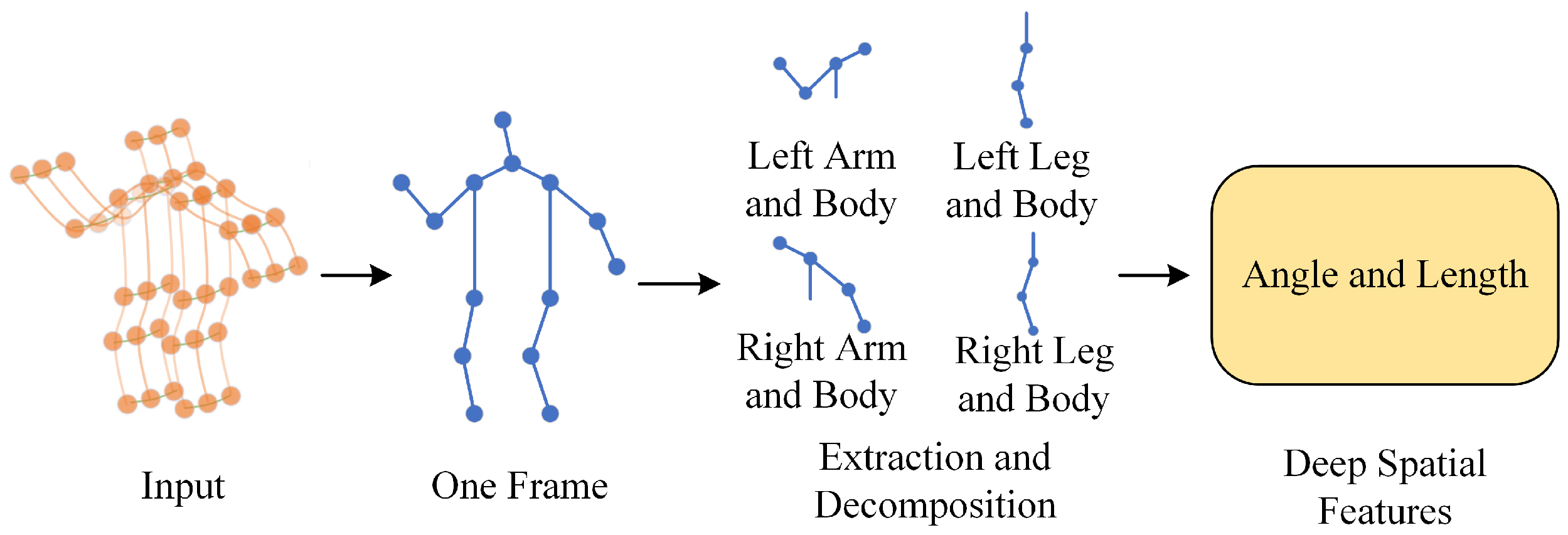
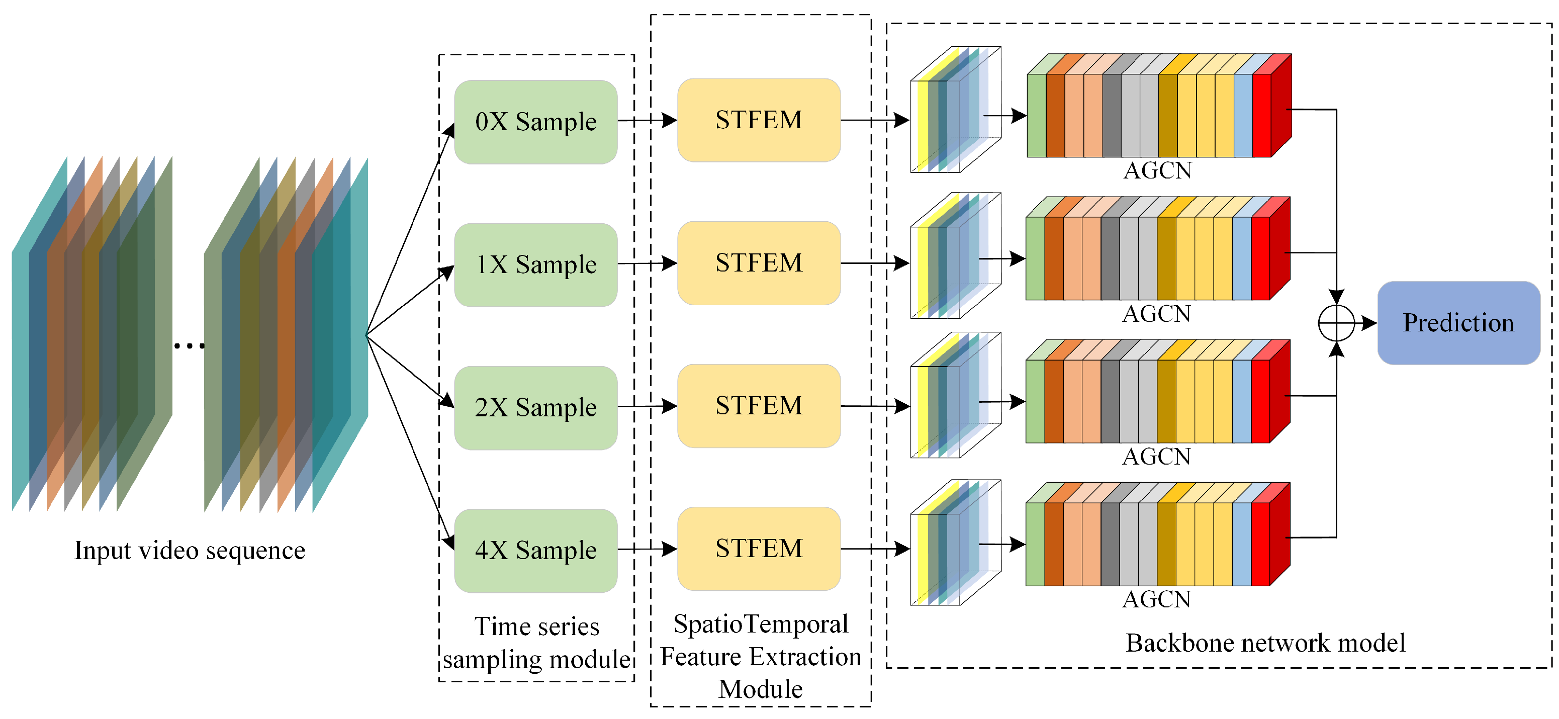
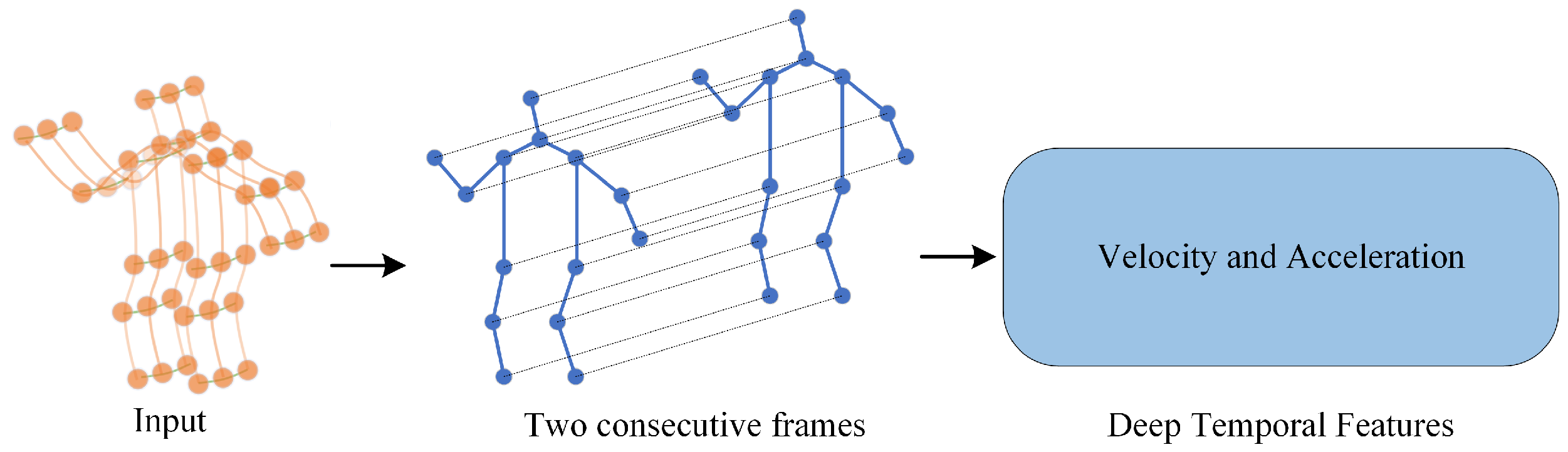
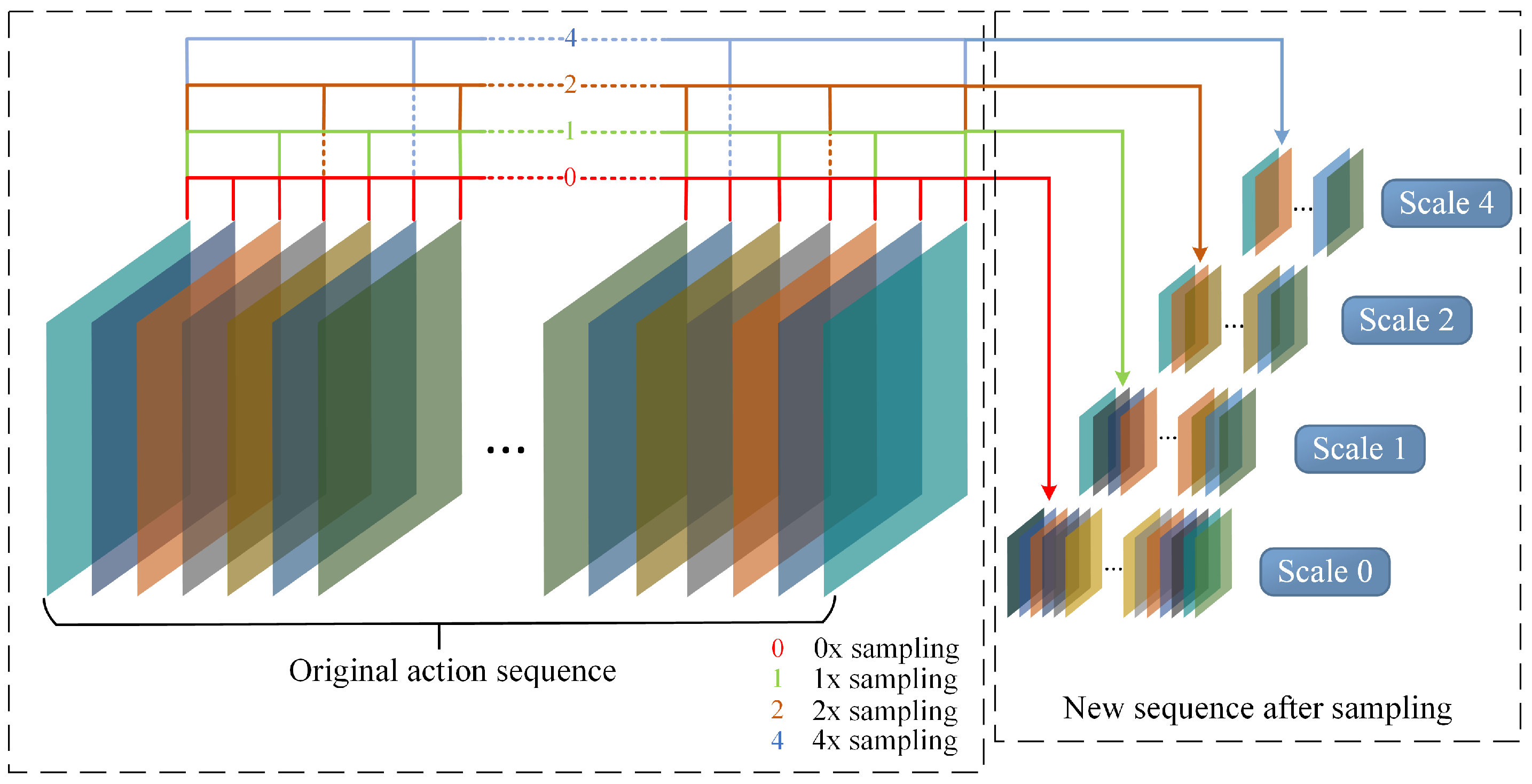
• Feature enhancement: In this paper, a multi-scale time-sampling module is proposed to obtain richer semantic information by varying the number of time frames. In addition, we combine the human skeleton map with the manipulator in robotics and propose a deep spatiotemporal feature extraction module. The module calculates the joint angle, the change of the joint angle, the angular velocity of the joint angle, and the acceleration of the joint angle in the human skeleton map, to make full use of the spatiotemporal features in the human skeleton data.
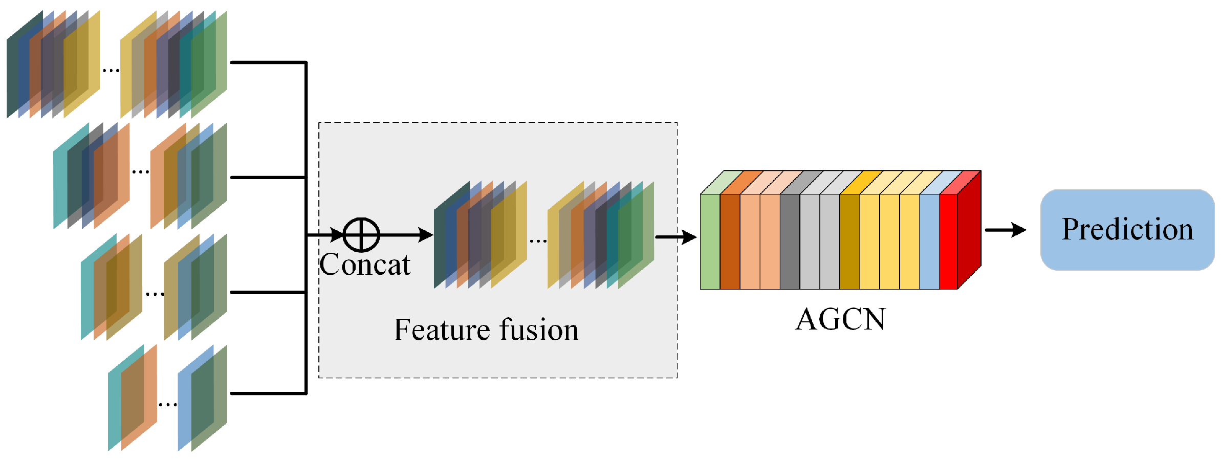
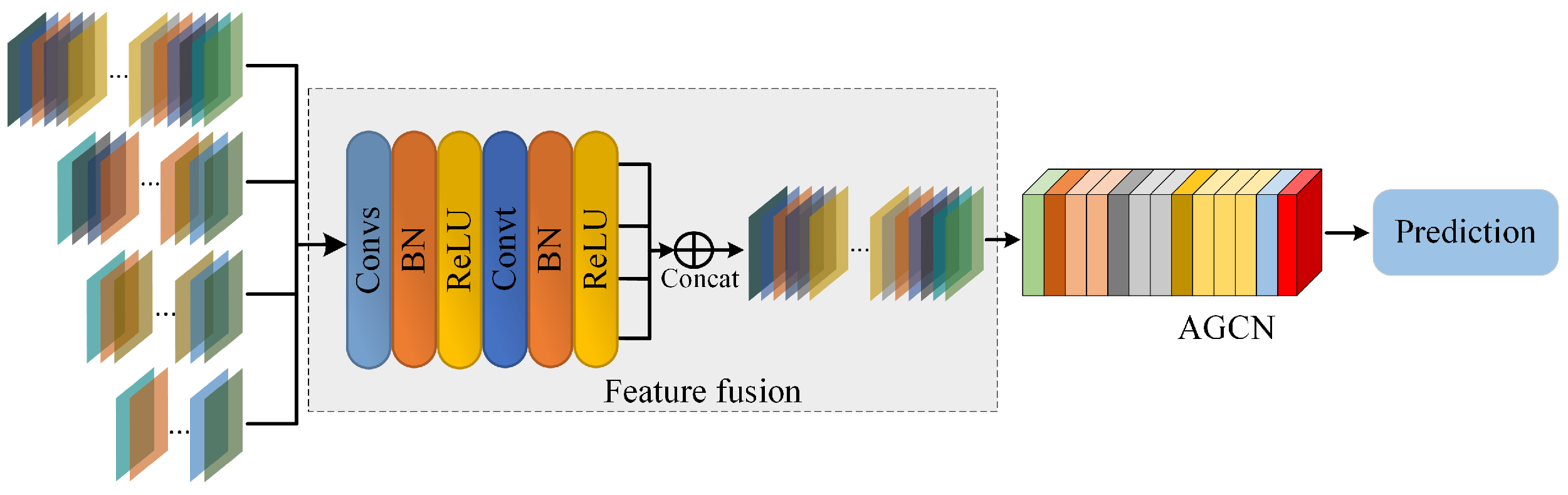
• Structure comparison: For the multi-scale deep spatiotemporal features proposed in this paper, we compare three different feature fusion methods. We introduce these three feature fusion methods in detail in Section 3. Experiments show that the decision-making level fusion method can achieve the best result for the model.

The remainder of this paper is organized as follows. Section 2 discusses some existing related works on skeleton-based action recognition and knowledge regarding robot manipulators related to this paper. In Section 3, on the basis of 2s-AGCN, we propose a deep spatiotemporal feature extraction module and three feature fusion methods. After comparing the advantages and disadvantages of the three methods, we concluded that the late fusion method was the most effective in this study. In Section 4, we give experimental proof for the relevant modules and feature fusion methods proposed in Section 3. In Section 5, we summarize the work of this paper and point out the directions of future work.

2. Related Works

In the field of action recognition with artificial intelligence as the mainstream method, the question of how to make full use of the temporal and spatial features in skeleton data is still a challenging problem. Control science involves finding the corresponding control output by establishing model parameters. Artificial intelligence is used to find the parameters of the model in the data. In essence, the main parameters used in these models may be universal. From the perspective of robot control, in this paper we aim to understand the parameters of motion recognition, strengthen its features, and propose a multi-flow network model based on these features.

2.1. Introduction to Manipulators in Robotics

In robot control, the basic theory is the motion control of rigid bodies, which is consistent with the meaning of recognizing bones in bone-based motion recognition. This section briefly introduces the four parameters of connecting rods and the motion of a rigid body.

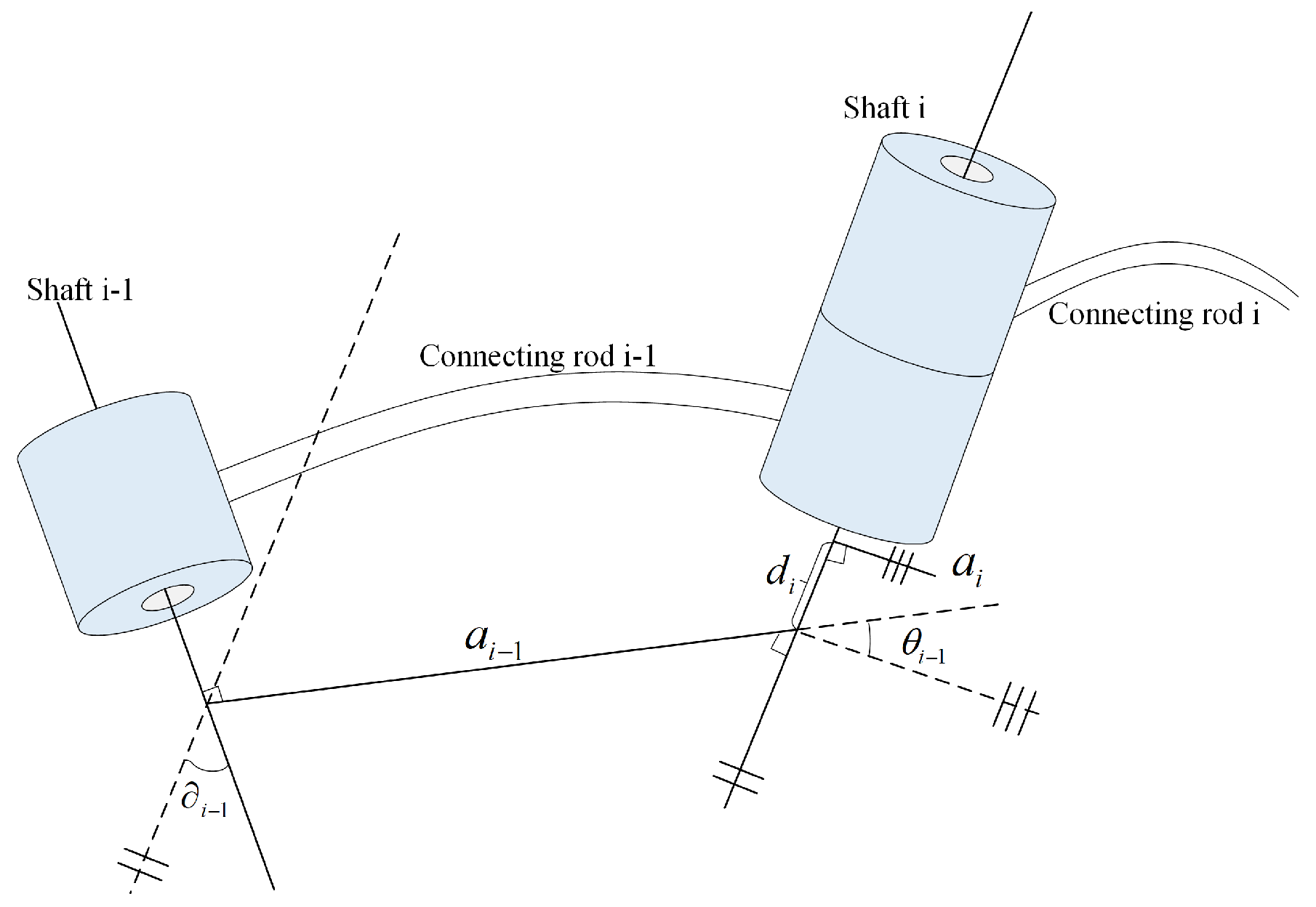
• Four parameters are related to connecting ros [14,15]. The connecting rods are numbered from the fixed base of the operating arm. The fixed base is connecting rod 0, the first movable connecting rod is 1, and so on. The connecting rod at the end of the operating arm is connecting rod n. In Figure 1, the joint axis $i-1$ and the joint axis i, the connecting rod $i-1$, and the connecting rod i are taken as examples to further illustrate the description of the joint–connecting rod connection.
  There is a common joint axis between two adjacent connecting rods. The distance along the common axis of two adjacent connecting rods can be described using a parameter called the connecting rod offset. The link offset on the joint axis i is marked as $d_i$. Another parameter is used to describe the angleof two adjacent connecting rods rotating around the common axis. This parameter is called the joint angle, which is recorded as ${\theta }_i$. Figure 1 shows the interconnected connecting rod $i-1$ and connecting rod i. According to the previous definition, ${\alpha }_{(i-1)}$ represents the connection relationship between two adjacent connecting rods. The first parameter is the directional distance from the intersection of the common vertical line ${\alpha }_{(i-1)}$ and the joint axis i to the intersection of the common vertical line ${\alpha }_{\left(i\right)}$ and the joint axis i, that is, the link offset $d_i$. A representation of the method of connecting rod offset $d_i$ is shown in Figure 1. When joint i is a moving joint, the link offset is $d_i$, which is a variable. The second parameter describing the connection relationship between adjacent connecting rods is the included angle formed by the rotation around the joint axis i between the extension line of ${\alpha }_{(i-1)}$ and ${\alpha }_{\left(i\right)}$, that is, the joint angle ${\theta }_i$, as shown in Figure 1. In the figure, the straight lines marked with double slashes and triple slashes are parallel lines. When joint i is a rotating joint, the joint angle ${\theta }_i$ is a variable.

  $${}^B{V}_Q=\frac{d^{B}Q}{dt}=\underset{\Delta t\to 0}{lim}\frac{{}^{B}Q(t+\Delta t){-}^{B}Q\left(t\right)}{\Delta t}$$

  (1)
  In the above formula, ${}^B{V}_Q$ represents the speed of point Q in coordinate system B, and ${}^{B}Q\left(t\right)$ represents the pose information of point Q in coordinate system B at time t. The orientation of coordinate system B relative to coordinate system A changes with time, and the rotation speed of B relative to A is expressed by vector ${}^A{\Omega }_B$, which indicates that an intuitive method can be used to calculate the point velocity. Two instantaneous quantities are used to represent the vector Q around ${}^A{\Omega }_B$. The rotation of B is observed from the coordinate system A. When analyzing the acceleration of a rigid body, the linear acceleration and angular acceleration can be obtained by deriving the linear velocity and angular velocity of the rigid body at any instant. The linear acceleration is shown in Equation (2) and angular velocity in Equation (3).

  $${}^B{V^{\prime }}_Q=\frac{d^B{V}_Q}{dt}=\underset{\Delta t\to 0}{lim}\frac{{}^B{V}_Q(t+\Delta t){-}^B{V}_Q\left(t\right)}{\Delta t}$$

  (2)

  $${}^A{{\Omega }^{\prime }}_B=\frac{d^A{\Omega }_B}{dt}=\underset{\Delta t\to 0}{lim}\frac{{}^A{\Omega }_B(t+\Delta t){-}^A{\Omega }_B\left(t\right)}{\Delta t}$$

  (3)
  From the introduction of relevant knowledge in the above operating arm, we can regard the two arms and two legs of the human body as operating arms. Therefore, we can calculate the angle, linear velocity and angular velocity, linear acceleration, and angular acceleration between adjacent joints.

2.2. Graph Convolutional Networks

A CNN can well process two-dimensional grid data such as images [16,17,18,19,20], but most of people’s daily life involves non-Euclideanspace data, so more and more people are engaged in research on GCNs [21,22,23,24,25,26]. There are two main methods used for GCNs: the spatial-based method and the spectral-based method. The spatial-based method directly convolutes the fixed points and their neighborhoods on the graph, and extracts and normalizes them according to the manually designed rules. Compared with the spatial-based method, the spectral-based method uses the eigenvalues and eigenvectors of the graph’s Laplace matrix. These methods perform graph convolution in the frequency domain by means of graph’s Fourier transform, which does not need to extract local connection regions from the graph at each convolution step. The work of this paper follows the space-based method. Yan et al. [5] proposed ST-GCN to directly model the skeleton data into a graphical structure, which does not need to design manual tasks or traversal rules, in order to obtain better performance than the previous methods. In the human skeleton diagram, the structure of the human limbs is very similar to that of the manipulator, so we considered introducing relevant variables in the manipulator to enrich the information in the human skeleton diagram. GCN is a method to deal with this non-Euclidean data.

3. Proposed Methods

In this chapter, we will elaborate on the deep spatiotemporal feature enhancement module, multi-scale time sampling strategy, feature fusion method, and backbone network model proposed in this paper.

3.1. Deep Spatiotemporal Feature Enhancement Module

When discussing the basic concepts of robotics, we observed that four variables are needed to describe a mechanical arm. Relatedly, the human skeleton map has a similar structure with the manipulator, but the manipulator is in three-dimensional space, and the human skeleton map can be regarded as being in a two-dimensional plane. In the process of movement, the movement speed of limbs varies with different actions. For example, in the two similar actions of falling and lying down, the duration of falling is shorter, whereas the duration of lying down is longer than that of falling. Therefore, it is necessary to calculate the variables such as speed and acceleration, angle, and angular acceleration. These variables can well reflect the unique features of people in different actions. This enriches the characteristics of human skeleton maps and is convenient for model learning.

3.1.1. Spatial Feature Extraction Module

The angle and angle variation of human joints can be used as the deep spatial features of an action recognition task based on bone data. This is associated with the fact that the structure of the mechanical arm in robotics is similar to that of human bone. Therefore, the relevant knowledge in the mechanical arm can be applied to human bone feature extraction. In the second section of this paper, we mentioned that four variables are needed to express the connecting-rod state of a mechanical arm in 3D space, whereas the human skeleton diagram considered in this paper only needs to consider 2D planes. Therefore, in the human skeleton graph, we remove the two variables of link angle and offset distance, and retain the two variables of link length and joint angle. Combined with the (x, y) coordinates given in the human skeleton dataset, it is easy to calculate the length of the bone and the angle between the bones. With these variables, we can easily represent the position of two arms and two legs of the human body. As shown in Figure 2, the deep spatial feature extraction module proposed in this paper inputs a group of action sequences and uses the coordinates of nodes to calculate the joint length and joint angle between each frame. In addition, we also increased the angle between the trunk and the large part of the arm and thigh to obtain the relative position of the arm and leg.

The rules for defining the angle extracted by the module are as follows. According to the coordinates of each node in the human bone dataset and its physical connection, the length of each bone and the angles between arms, legs, and trunk are calculated. When the degree of the node is 1, the node has only one edge and there is no need to calculate the angle; when the degree of a node is 2, a node connects two edges and only an angle less than 180° needs to be calculated; when the degree of a node is 3, a node connects three edges and three angles need to be calculated; similarly, nodes with a degree of 4 need to calculate four angles. Figure 3 shows an example of a human skeleton data label graph.

Taking node 5 in Figure 3 as an example, node 5 is located in the left arm of the human body, and its degree is 2. It is necessary to calculate an angle formed between its two bones. Similarly, the included angles between other arms, legs, and trunk are also calculated one by one through Formula (4). Taking node 5 as an example, one can express the included angle calculation formula as shown in Equation (4).

$${\theta }_5=arccos\left[\frac{(x_4-x_5)\times (x_7-x_5)+(y_4-y_5)\times (y_7-y_5)}{\sqrt{{(x_4-x_5)}^2+{(y_4-y_5)}^2}\times \sqrt{{(x_7-x_5)}^2+{(y_7-y_5)}^2}}\right]$$

(4)

‘X’ and ‘Y’ in the above formula represent the abscissa and ordinate of the node, and their subscripts represent the sequence numbers of the nodes, ${\theta }_5$ represents the angle on the node labeled 5. The calculation formula of a defined length is shown in Formula (5).

$$\left|L_1\right|=\sqrt{{(x_1-x_2)}^2+{(y_1-y_2)}^2}$$

(5)

$\left|L_1\right|$ represents the length of the bone between node 1 and node 2 in the above formula, and its subscript represents the label of the first bone. According to the above method of extracting the angle between bone length and bone, the angles and lengths between all bones in a single frame are extracted to obtain the deep space feature matrix.

3.1.2. Time Feature Extraction Module

Inspired by the knowledge on rigid body motion in manipulators, we suggest that the human skeleton can also be used to calculate linear velocity and angular velocity, linear acceleration, and angular acceleration. Here, we simplify the linear velocity and linear acceleration as the linear velocity and linear acceleration on the node, and the angular velocity and angular acceleration as the angular velocity and angular acceleration between adjacent joints. Based on the characteristics of human skeleton data, we can rewrite Equation (1)–(3). The deep time feature extraction module is shown in Figure 4.

We simplify the calculation of linear velocity and obtain the differential of the abscissa and the ordinate of each node at time t and time t + 1. The result of the differential can represent the linear velocity of the node at time t, as shown in Equation (6).

$$V=\frac{d{J}^m}{dt}=\underset{\Delta t}{lim}\frac{J^m(t+\Delta t)-J^m\left(t\right)}{\Delta t}$$

(6)

In the above formula, $J^m$ represents the (x, y) coordinates on the m-th node, $\Delta t$ takes the value of 1. For the linear acceleration, according to Equation (2), we calculate the differential of the online velocity of each node at time t to obtain the linear acceleration of the node at time t, as shown in Equation (7).

$$\dot{V}=\frac{dV}{dt}=\underset{\Delta t}{lim}\frac{V(t+\Delta t)-V\left(t\right)}{\Delta t}$$

(7)

Definition V represents the linear velocity on the node, $\dot{V}$ represents the linear acceleration on the node, and $\Delta t=1$. Because the human skeleton data are extracted frame-by-frame from the video, which is discrete data, we specify $\Delta t=1$. So the calculation formulas of linear velocity and linear acceleration are as shown in Equations (8) and (9):

$$V=J^m(t+1)-J^m\left(t\right)$$

(8)

$$\dot{V}=V(t+1)-V\left(t\right)$$

(9)

Similarly, according to the characteristics of human bones, the angular velocity and angular acceleration on human bones are calculated, and $\Omega$ is defined to represent the angular velocity on joints, whereas $\dot{\Omega }$ represents the angular acceleration on joints. The angular velocity and angular acceleration are calculated from the angle extracted from the deep spatial features. The calculation principle is similar to that of the linear velocity on the node, and it is specified as $\Delta t=1$, the calculation formula is shown in Equations (10) and (11).

$$\Omega =\theta (t+1)-\theta \left(t\right)$$

(10)

$$\dot{\Omega }=\Omega (t+1)-\Omega \left(t\right)$$

(11)

3.2. Time Multi-Scale Sampling Module

At present, most action recognition methods based on deep learning process all actions according to a single fixed time scale, but we believe that the time span of an overall action is changeable, the degree of change of action between each frame is also different, and there is inclusion between action meanings. It is not optimal to use a single time scale to deal with the problem of action recognition. Therefore, we propose an equal-interval-time multi-scale sampling strategy. As shown in Figure 5, we extract the multi-scale action sequence using a certain number of frames. We believe that the multi-scale action sequence extracted after a certain number of frames can contain more semantic information, and then the multi-scale deep spatiotemporal features are calculated using the deep spatiotemporal feature extraction module. When we select the interval frames, we find that the duration of some actions is short. If the interval frames are too numerous, the action sequence of this scale will lose its original semantic information and the meaning of the action itself will be lost. Therefore, we select 0, 1, 2, and 4 when we select the interval frames.

3.3. Selection of Feature Fusion Methods

Because so many features are extracted from skeleton data, the question of how to deal with these features has also become a key part of our work. In the process of multi-scale feature fusion, the time of fusion is an important consideration. For different fusion periods, we tried three feature fusion methods: early fusion and late fusion, also known as feature fusion and decision-making level fusion. Early fusion, also known as feature fusion, refers to a fusion method immediately after multi-scale feature extraction. Late fusion is also called decision-making level fusion, which refers to making decisions (classification or regression) at each scale after that. The fused part in Figure 6, Figure 7 and Figure 8 is marked with a dashed box. By comparing the results of the model under three feature fusion methods, the optimal fusion method was obtained. The first two feature fusion methods corresponded to early fusion, and the third fusion method corresponded to late fusion. We carried out two processes for feature layer fusion. The first method is shown in Figure 6. In this method, the features of four time scales are directly spliced according to the dimensions of keyframes to obtain a feature matrix with dimensions of (3, M, N, 2), where M represents the number of keyframes and N represents the number of key points. We take this feature matrix as the input matrix of AGCN, and finally, AGCN is used to obtain the classification results. The second method is shown in Figure 7. Firstly, the features of four-time scales are passed through a graph convolution layer and a ReLU activation function layer to increase the nonlinear expression ability of the features, and then spliced according to the dimensions of the keyframe. Similarly, a feature matrix with dimensions (3, M, N, 2) is obtained. We take this feature matrix as the input matrix of AGCN. Finally, the classification results are obtained by means of the AGCN. The third method is shown in Figure 8. We respectively input the features of four different time scales into AGCN to obtain the scores of four classifications. Finally, the scores of these four classifications are added in equal proportion to obtain the final result. The fusion method is shown in Equation (12).

$$S_{all}=0.25S_0+0.25S_1+0.25S_2+0.25S_4$$

(12)

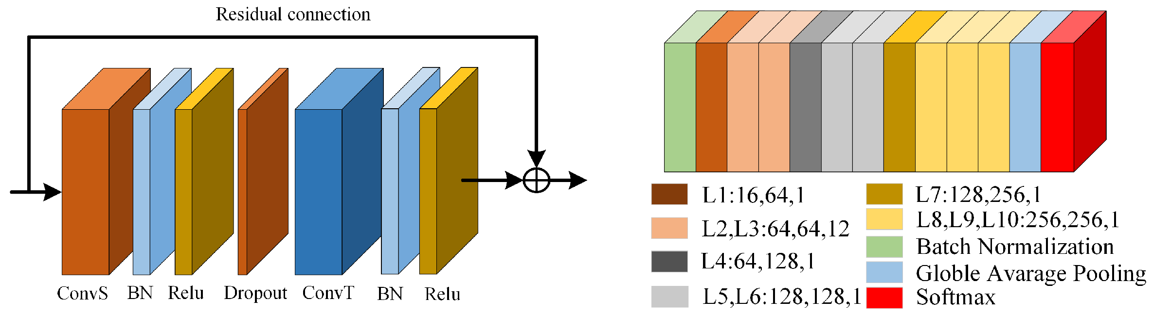
3.4. Skeleton Action Recognition Algorithm Based on Multi-Scale Deep Spatiotemporal Features

The basic model of this paper comes from 2s-AGCN. The AGCN shown in Figure 9 is a multilayer adaptive graph convolution network model, which optimizes the network topology and other network parameters in an end-to-end manner. This graph has uniqueness for different layers and different samples and can adapt to the model very flexibly. At the same time, a residual connection is added to the model to ensure the stability of the original model. More specifically, in the spatial dimension, to make the graph adapt to different samples and graph structures, we use the iterative formula shown in Equation (13).

$$f_{out}=\sum _K^{K_v}{W}_k{f}_{in}(A_k+B_k+C_k)$$

(13)

$K_v$ represents the kernel size of spatial latitude. According to the division rules of subgraphs, we set $K_v=3$, $W_k$ is the weight matrix, and $A_k$ is an N × N, which represents the physical structure of the human body. $B_k$ is also an adjacency matrix of N × N, but $B_k$ has no specific constraints on the inner value, which means that the graph is completely learned from the training data. In the data-driven task, we can completely learn the graph from the target task, considering that the value in $B_k$ can be any value, which can represent not only the physical structure of the human body but also the connection strength between adjacent nodes. $C_k$ can represent a data correlation graph, which can learn a unique graph for each sample. To determine whether there is a connection between two adjacent nodes and how strong the connection is, we use the normalized Gaussian function to calculate the similarity of the two nodes, as shown in Equation (14).

$$f(v_i,v_j)=\frac{e^{\theta {\left(v_i\right)}^T\varphi \left(v_j\right)}}{{\displaystyle \sum _{j=1}^N}{e}^{\theta {\left(v_i\right)}^T\varphi \left(v_j\right)}}$$

(14)

Here, N represents the sum of all nodes. We use the point product to calculate the similarity of two nodes in the embedded space. $C_k$ is a similarity matrix of $N\times N$; we normalize the value to be between 0 and 1. This is consistent with the time dimension in ST-GCN in the time dimension. Every BN layer and Relu layer is connected behind each spatial graph convolution and time graph convolution.

For the multi-scale deep spatiotemporal features proposed in this paper, we tried three different feature fusion methods. In the experiment discussed in Section 4, we concluded that the fusion effect at the decision level is the best. Therefore, when introducing the model in this section, we only introduce the third method in detail. Figure 10 depicts the skeleton action recognition model based on multi-scale deep spatiotemporal features proposed in this paper. Firstly, an action sequence is given, and four groups of actions with different scales are obtained after multi-scale time sampling. Then, the deep spatiotemporal feature extraction module (STFEM) is used to extract the deep spatiotemporal features of actions of four scales, and then the spatiotemporal features of these four scales are sent to the AGCN, respectively. After the Softmax classifier is applied, four different classification scores are obtained, and then the four classification scores are added in equal proportion to obtain the final classification result.

4. Experimental Results and Analysis

In this section, we analyze the effectiveness of the deep spatiotemporal feature extraction model proposed in this paper through experiments and compare the three feature fusion mechanisms, in order to analyze their advantages and disadvantages. The method was tested on two large datasets in the field of action recognition, Kinetics, and NTU-RGB+D. The test results are compared with the results of 2s-AGCN to confirm the effectiveness of the model proposed in this paper, and then the model proposed in this paper is compared with the existing SOTA.

4.1. Datasets

NTU-RGB+D [27] is the largest dataset with 3D Node annotation in relation to human motion recognition tasks. This dataset contains 60 motion categories and a total of 56,000 human motion video clips. All these clips were completed by 40 volunteers in a specific laboratory. It uses three Kinect V2 cameras with the same height but different angles to capture information at the same time, with angles of $-45$°, 0°, and 45°. This dataset obtains the position information, marked by 3D nodes on each frame, through the Kinect depth sensor. Each character in each skeleton sequence has 25 nodes, and there are only two characters in each segment at most. The author of NTU-RGB+D proposes to use two indicators: (1) the Cross Subject (X-Sub) evaluation index; in this evaluation index, the dataset is divided into the training set and verification set according to the person’s ID. the training set has 40,320 segments and the verification set has 16,560 segments; (2) the Cross View (X-View) evaluation index, in which the evaluation index is divided according to the number of cameras. The information captured by cameras 2 and 3 is divided into training sets, and the information captured by camera 1 is divided into verification machines, including 37,920 segments in the training set and 18,960 segments in the verification set. The evaluation indexes used in this paper follow the above two indexes, and the recognition accuracy of top-1 on the two datasets is given.

Kinetics [28] is a large human action dataset, which contains 400 action categories. These actions are depicted in videos obtained from YouTube. Each action category has at least 400 video clips, and each video clip includes at least 10 s. These actions include the interaction between people and objects, such as playing musical instruments, as well as interactions between people, such as shaking hands. However, this dataset only provides video without skeleton data. Therefore, in this study we used the OpenPose [29] toolbox to estimate the positions of 18 joints in each frame of the video clips. We selected two people for multiplayer editing according to the average joint confidence. We used their published data to evaluate our model. The dataset was divided into a training set and a verification set, in which the training set included 240,000 fragments and the verification set included 20,000 fragments. According to the evaluation method in Kinetics, we trained the model on the training set and obtained the top-1 and top-5 accuracy in the verification set. In the dynamics skeleton dataset, the node labels were: 0—nose, 1—neck, 2—right shoulder, 3—right elbow, 4—right wrist, 5—left shoulder, 6—left elbow, 7—left wrist, 8—right hip, 9—right knee, 10—right ankle, 11—left hip, 12—left knee, 13—left ankle, 14—right eye, 15—left eye, 16—right ear, and 17—left ear.

4.2. Training Details

All the experiments in this paper werw based on the Pytorch framework and run on a server using a 9th generation Intel CPU, 64 G memory, and two NVIDIA 2080ti GPUs. According to the batch size, which was set to 16 in this paper, the operation occupancy rate of the two graphics cards was between 85% and 90%. The optimization algorithm used the stochastic gradient descent (SGD) algorithm. Its momentum was set to 0.9 and its batch size was set to 16. The loss function used was the cross-entropy function. The weight decay was set to 0.0001; the initial learning rate was set to 0.1. For the NTU-RGBD dataset, there are at most two people in each sample of the dataset. If the number of bodies in the sample was less than 2, we used a value of zero for the second body. The maximum number of frames in each sample is 600. For samples with less than 300 frames, we repeated the samples until they reached 600 frames. The learning rate was set as 0.1 and this was divided by 10 at the 30th epoch and 40th epoch. The training process was ended at the 50th epoch [6,7]. For the Kinetics-Skeleton dataset, the size of the input tensor of Kinetics was set the same as [6], containing 150 frames with two bodies in each frame. We performed the same data-augmentation methods as in [6]. In detail, we randomly chose 300 frames from the input skeleton sequence and slightly disturbed the joint coordinates with randomly chosen rotations and translations. The learning rate was also set as 0.1 and was divided by 10 at the 45th epoch and 55th epoch. The training process ended at the 65th epoch [6,7]. To increase the reliability of the experimental results, during the training process, we repeated the process 10 times for the three feature fusion methods noted in Section 4.3 and the ablation experiments noted in Section 4.4 and took the average value of the results of these 10 experiments as the final results of all experiments in this paper.

4.3. Effectiveness Comparison of Time Multi-Scale Modules

In this paper, we propose a time multi-scale sampling module. First, we preprocessed the dataset and divided the dataset into four scales according to the time sampling strategy described in Section 3. We named them scale 0, scale 1, scale 2, and scale 4, respectively. Secondly, we directly input the features of four times scales into the AGCN. To make the experimental results more fair, we took the node flow in the dual flow adaptive graph convolution network as a reference and experimented only on a single graph from the adaptive convolution model. As shown in

Table 1. Comparison of the accuracy of features of different time scales on the NTU-RGB+D and Kinetics datasets.

Methods	Cross-View%	Cross-Subject%	Kinetics%
Scale 0 (J-Stream)	93.1	86.3	34.0
Scale 1	93.9	87.1	35.0
Scale 2	92.7	86.2	33.2
Scale 4	91.5	85.2	33.5

, we compared the effects of the characteristics of four different time scales on the same model on NTU-RGB+D and the dynamics datasets.

The result of the basic network used in this paper for the Kinetics dataset was only 34%. The effect of our time multi-scale sampling strategy on scale 1 was 1% better than that of the basic network. As for why the accuracy of the kinetic dataset was very low, we suspect that it is because the types of datasets were increasing. The number of classification types in the Kinetics dataset used in this paper is up to 400, whereas the NTU-RGB+D dataset has only 60 classification types. From the results shown in Table 1, it can be seen that the multi-scale sampling module proposed in this paper achieved the best effect at an interval of one frame (scale 1) and exceeded that of J-Stream (one of AGCN’s branches). However, the effect achieved on the adaptive graph convolution model’s scale 2 and scale 4 decreased gradually. For NTU-RGB+D dataset and the Kinetics dataset, scale 1 produced 0.8%, 0.8%, and 1% higher accuracy than scale 0, respectively, but scale 2’s results were 0.4%, 0.1%, and 0.8% lower than those of scale 0, and scale 4’s results were 1.6%, 1.1%, and 1.5% lower than those of scale 0. After this analysis, we believe that although the time multi-scale module can obtain a larger receptive field by spacing a certain number of frames, a side effect is that it loses part of the semantic information, resulting in a decline in the recognition performance of the model. However, to make up for this part of the lost semantic information, we have introduced the deep spatiotemporal feature module. This module is introduced in detail in Section 3.3, and the experimental results of the module are given in Section 4.5.

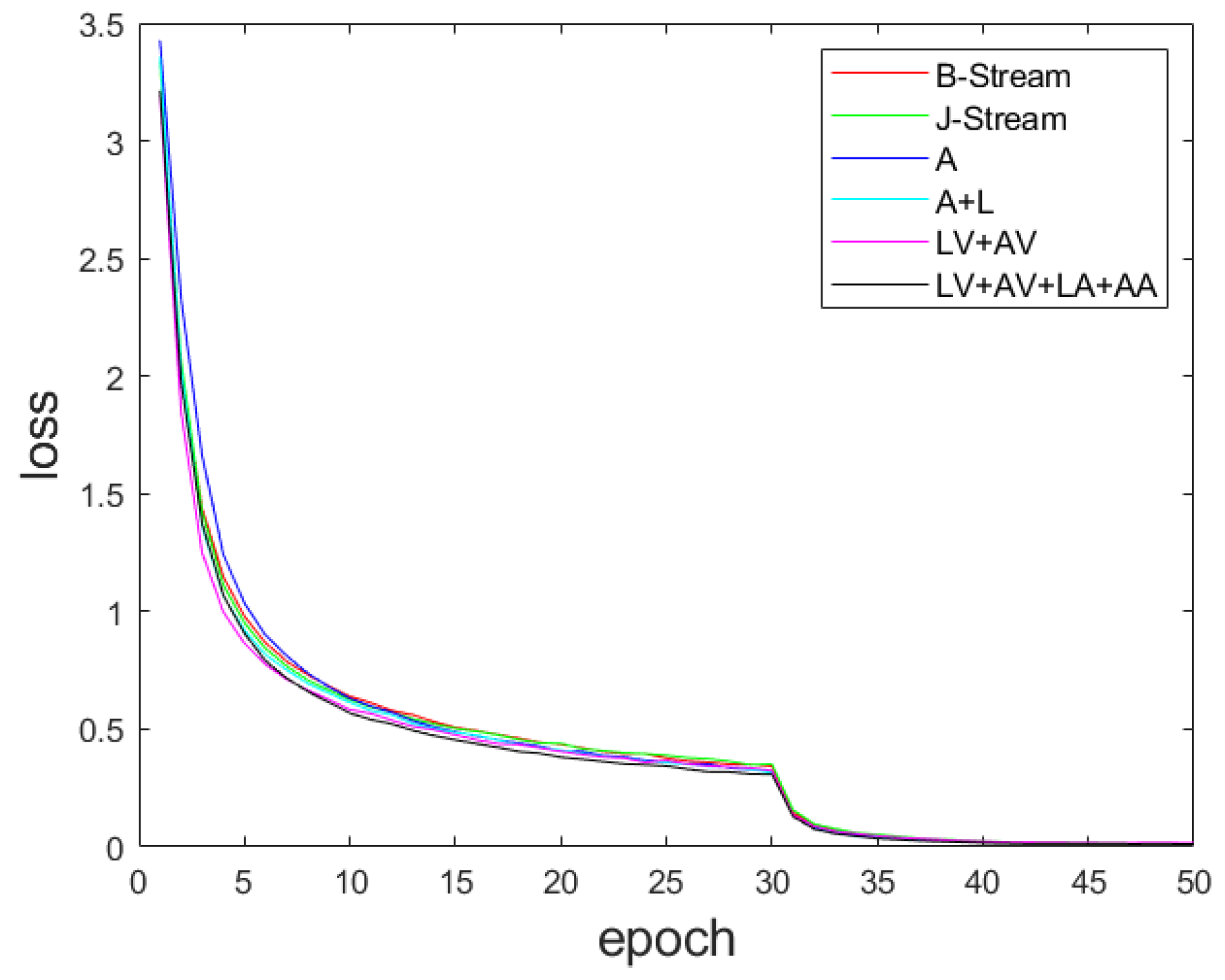
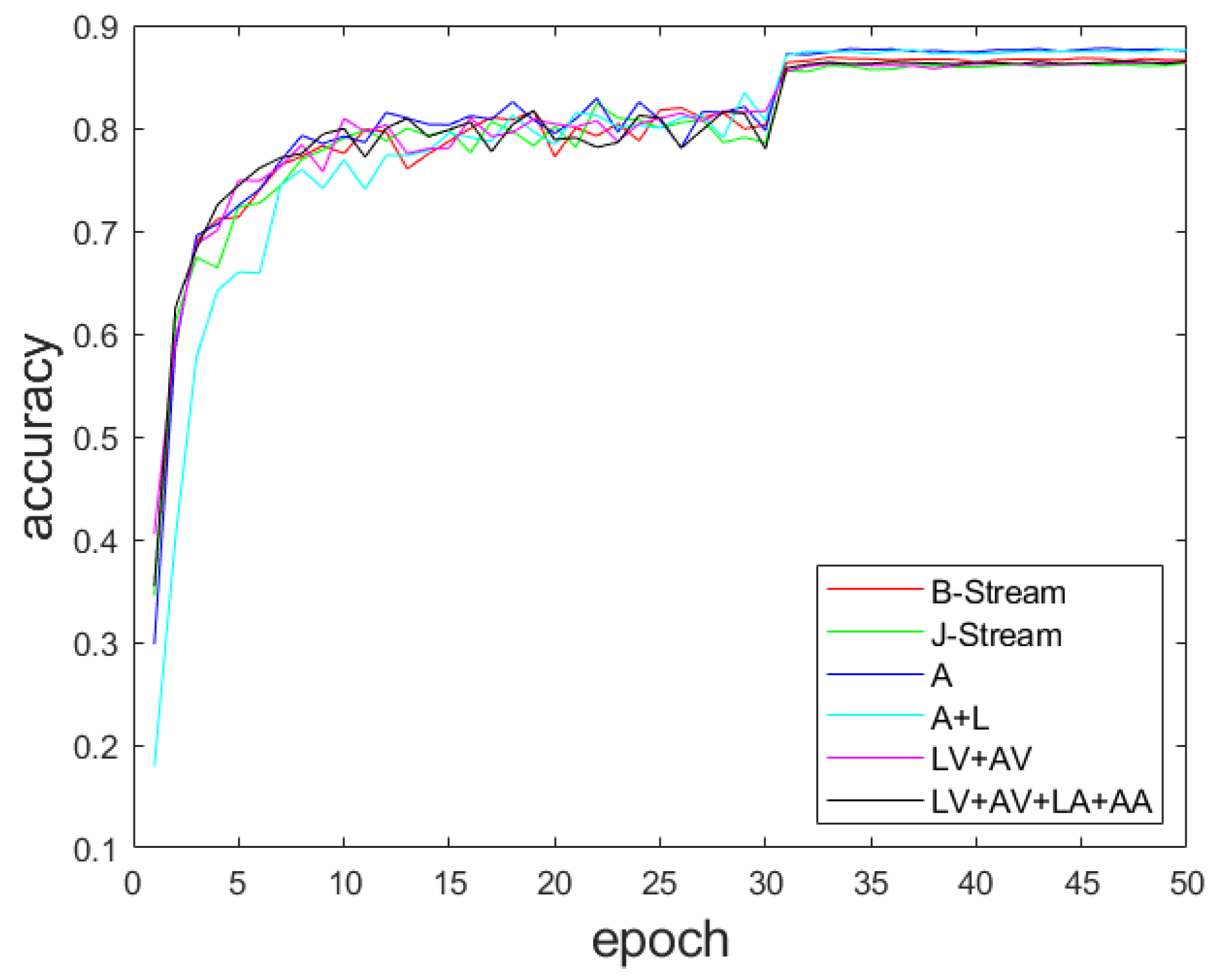
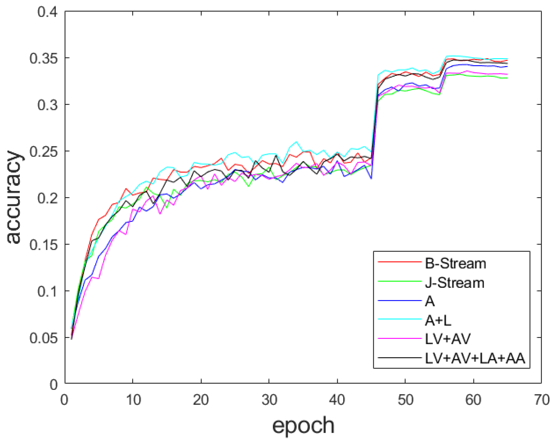
4.4. Effectiveness Analysis of Deep Spatiotemporal Feature Module

To verify the effectiveness of the module proposed in this paper, we compared the B-Stream and J-Stream in the 2s-AGCN with the multi-stream adaptive graph convolution network proposed in this paper. To control the same variables, we did not sample the action sequence. We compared the spatial and temporal features, respectively, and verified the effectiveness of the module proposed in this paper by controlling different inputs. The comparison results are shown in

Table 2. Comparison between the accuracy of 4-stream features extracted using the spatiotemporal feature extraction module under the same time sampling conditions and the accuracy of the dual-stream features of the original 2s-AGCN.

Methods	Cross-View%	Cross-Subject%	Kinetics%
B-Stream	93.3	86.7	34.3
J-Stream	93.1	86.3	34.0
A	93.5	87.5	32.8
A + L	93.7	87.6	34.9
LV + AV	93.2	86.4	33.2
LV + AV + LA + AA	93.8	86.5	34.7

. We used A to represent an angle, L to represent length, LV to represent linear velocity, AV to represent angular velocity, LA to represent linear acceleration, and AA to represent angular acceleration. The results presented in Table 2 show that the accuracy of the NTU-RGB+D and Kinetics datasets was improved after adding the deep spatiotemporal features. It can be seen that the deep spatiotemporal features module was more effective in improving the accuracy of the model. In the CV index of the NTU-RGB+D dataset, the use of ‘LV + AV + LA + AA’ as the input feature has the best accuracy, reaching 93.8%, and the effects of other features on this evaluation index were not very different. On the CS index, the use of ‘A + L’ as the input features achieved the best effect, reaching 87.6%, 1.3% ahead of ‘J-Stream’; ‘A + L’ also performed well on the Kinetics dataset, leading ‘J-Stream’ by 0.9%. In terms of model training speed, it can be seen in Figure 10 that although the number of features is increased in our proposed method, there is no obvious disadvantage in speed.

The original network we used was 2S-AGCN [6], and the model’s training method was also consistent with that of the basic network. The turning point of the training curve in Figure 11, Figure 12, Figure 13, Figure 14, Figure 15 and Figure 16 was caused by the decay of the learning rate. At the beginning of the training process, using a large learning rate (0.1) can accelerate the model convergence. Yan et al. [5] and Shi et al. [6] have proven the effectiveness of learning rate decay in training motion recognition models. With the progress of the training process, the learning rate will be gradually reduced to help find the optimal solution and reduce the fluctuation of the loss function. Our experiments show that the use of learning rate decay in the training process has a certain effect in the case of our proposed model.

In the process of model training, we recorded the loss value and accuracy of each epoch. In Figure 11, Figure 12, Figure 13, Figure 14, Figure 15 and Figure 16, the red line represents the ‘B-Stream’, the green line represents the ‘J-Stream’, the blue line represents the input feature ‘A’, the green line represents the input feature ‘A + L’, the purple line represents the input feature ‘LV + AV’, and the black line represents ‘LV + AV + LA + AA’. As can be seen in Figure 10, after adding the deep spatiotemporal feature extraction module, the effect of the model has been further improved based on the original two streams’ adaptive graph convolution. As can be seen in Figure 11, Figure 12, Figure 13 and Figure 14, on the NTU-RGB+D dataset, the model with six branches begins to converge after the 32nd epoch, the loss value of the converged model is less than 0.1, and the fluctuation is small. Furthermore, the accuracy gradually tends to be stable after 32 epochs. We can see in Figure 11 and Figure 13 that when ‘LV + AV + LA + AA’ and ‘A + L’ are used as input characteristics, the loss of the two branch models is at the lowest value in all branches in the 10th epoch, and the loss is kept at the lowest state until the end of training. As can be seen in Figure 15, on the dynamics dataset, the loss value of the ‘A + L’ branch reaches the minimum of all the branches at the 10th epoch and remains in a steadily declining state until the end of training.

4.5. Comparison of Multi-Scale Feature Fusion Methods

In this paper, multi-scale deep spatiotemporal features are proposed. We considered how to make better use of these features. Therefore, we proposed three feature fusion methods based on two approaches: early fusion and late fusion. Early fusion is also called feature fusion, and refers to a fusion method conducted immediately after multi-scale feature extraction. Late fusion is also referred to as decision-making level fusion. It refers to the integration after making decisions (classification or regression) at each scale. In this study, methods 1 and 2 corresponded to early fusion and method 3 corresponded to late fusion. Method 2 had one more graph convolution layer and activation function layer than method 1, in order to increase the nonlinear expression ability of the data. The same problem can be solved using different algorithms. The quality of an algorithm will affect the efficiency of the algorithm and even the program. The purpose of algorithm analysis is to select the appropriate algorithm and improve the algorithm. We evaluated the time complexity of the algorithm. The adaptive graph convolution algorithm had the same algorithm execution flow as the algorithm in this paper, and only uses a for a loop once. The feature fusion of methods 1 and 2 occurs in the early stage, so the time complexity of methods 1 and 2 is $Time{s}_c$∼$O\left(E^B\right)$, where $E^B$ is the B power of E, E is the number of training epochs, and B is the minimum of the minibatch. Since four adaptive graph convolution algorithms are used in the later stage of feature fusion in method 3, the time complexity of method 3 is $Time{s}_c$∼$O\left(4E^B\right)$; four means that there are four identical adaptive graph convolution neural networks that process four different scale features at the same time. To verify the advantages and disadvantages of the three feature fusion methods proposed in this paper, we compared the training time and classification accuracy of the three models on NTU-RGB+D and Kinetics datasets, respectively. The comparison results are shown in

Table 3. Comparison of the accuracy and training time of three methods on the NTU-RGB+D and Kinetics datasets.

	Cross-View %
Methods	Accuracy (%)	Times(h)
Method 1	90.6	30.8
Method 2	91.5	30.9
Method 3	95.5	98
	Cross-Subject %
Methods	Accuracy (%)	Times(h)
Method 1	86.5	35
Method 2	87.0	35.2
Method 3	89.5	106
	Kinetics %
Methods	Accuracy (%)	Times(h)
Method 1	32.0	24.8
Method 2	32.1	25
Method 3	37.1	79

.

As can be seen in Table 3, the accuracy of method 1 and method 2 on the two datasets was not as high as that of method 3. In terms of the CV index of the NTU-RGB+D dataset, the accuracy of method 3 was 4% and 4.0% higher than that of method 1 and method 2, respectively. In terms of the CS index, the accuracy of method 3 was 3.0% and 2.5% higher than that of method 1 and method 2, respectively. On the Kinetics dataset, the accuracy of method 3 was 5.1% and 5.0% higher than that of method 1 and method 2. However, in terms of training time, method 3 needs to train the features of four-time scales four times, so the training time was longer than those of the first two methods, but the results were greatly improved. We believe that the reason for the low accuracy of methods 1 and 2 in these two methods is that it is difficult to represent the time synchronization between multi-scale features in the early fusion stage. Because the representation, distribution, and density of various scales may be different, only a simple connection between attributes may ignore the unique attributes and correlations of each scale. Furthermore, this may cause redundancy and data losses between data. Early fusion also requires the fused features to be represented in the same format before fusion. With the increase in the number of features, it is difficult to obtain cross-correlation between these features. Method 3 uses the corresponding models to train the features of four different scales and then fuses the output results of the four models. Compared with methods 1 and 2, method 3 can handle simple data asynchrony, but it is obvious from Table 1 that the learning process of method 3 is time-consuming. In order to verify the engineering value of this paper, according to the distribution of action frames, we selected the interval with the most concentrated action distribution, and randomly selected five actions as the test. As shown in

Table 4. Comparison of the testing times of five examples of three methods on the NTU-RGB+D dataset.

Action Type	Frame	Method 1(s)	Method 2(s)	Method 3(s)
A10: Clapping	69	1.4	1.4	1.5
A7: Throw	86	1.5	1.5	1.6
A27: Jump up	87	1.5	1.5	1.6
A4: Brush air	99	1.5	1.5	1.6
A1: Drink water	103	1.5	1.5	1.6

below, we recorded the test time and accuracy. It can be seen from Table 4 that the three methods have certain engineering value.

4.6. Comparison with Existing State-of-the-Art Network

We compared the results of the model using method 3 with the existing state-of-the-art network model. We compared the results of this model with those of mainstream skeleton-based action recognition methods on the Kinetics dataset and NTU-RGB+D dataset. The comparison results are shown in

Table 5. Comparison of accuracy between SOTA methods using the Kinetics dataset.

Action Type	Date	Top-1(%)	Top-5(%)
Feature Encoding [31]	2015	14.9	25.8
Deep LSTM [32]	2016	16.4	35.3
Temporal ConvNet [33]	2017	20.3	40.0
ST-GCN [5]	2018	30.7	52.8
2S-AGCN [6]	2019	36.1	58.7
GCN-NAS [30]	2020	37.1	60.0
1s-AAGCN [34]	2020	36.0	58.4
2s-AAGCN [34]	2020	37.4	60.4
4s-AAGCN [34]	2020	37.8	61.0
MST-AGCN (ours)	-	37.1	61.0

and

Table 6. Comparison of accuracy between SOTA methods using the NTU-RGB+D dataset.

Methods	Date	Cross-View (%)	Cross-Subject (%)
Deep LSTM [32]	2016	67.3	60.7
Temporal ConvNet [33]	2017	83.1	74.3
VA-LSTM [35]	2017	87.6	79.4
Two-stream CNN [36]	2017	89.3	83.2
GCA-LSTM [37]	2017	82.8	74.4
ARRN-LATM [38]	2019	89.6	81.8
MANs [39]	2018	93.2	83.0
ST-GCN [5]	2018	88.3	81.5
DPRL + GCNN [40]	2018	81.5	83.5
2S-AGCN [6]	2019	95.1	88.5
RA-GCN [41]	2020	93.6	87.3
MV-IGNet [42]	2020	96.3	89.2
MST-AGCN (ours)	-	95.5	89.5

. It can be seen in Table 5 and Table 6 that the deep spatiotemporal feature extraction module proposed in this paper showed an improvement to a certain extent on the basic 2s-AGCN approach. On the Kinetics dataset, top-1 was improved by 1% and top-5 by 2.3%. The CV evaluation index in the NTU-RGB+D dataset was increased by 0.4%, and the CS evaluation index was increased by 1%. Compared with other mainstream models, our model showed advantages and disadvantages in relation to the Kinetic dataset. For example, the results of our model and GCN-NAS [30] on top-1 were the same but the results of our model on top-5 were still 1% higher. Similarly, compared with 2s-AAGCN, the results of our model on top-1 was slightly lower than those of 2s-AAGCN, but it was still 0.6% higher on top-5. Compared with 4s-AAGCN, the results of our model on top-1 were 0.7% lower than those of 4s-AAGCN, but the results on top-5 were the same. For the NTU-RGB+D dataset, compared with the more advanced MV-IGNet, the accuracy of our model was 0.8% less in terms of the CV index, but in terms of the CS index, our model’s results were slightly higher than those of MV-IGNet.

5. Conclusions

In human–computer interactions and other fields that require the use of action recognition methods, it is necessary to recognize actions accurately and quickly to obtain a better experience. In the process of practical experience, we find that the time spans of some actions are different, and there may be an inclusion relationship between action semantics. Based on 2s-AGCN, in this paper we have proposed a skeleton action recognition algorithm based on multi-scale depth spatiotemporal features. The algorithm adopts a multi-scale time sampling module and a depth spatiotemporal feature extraction module, which enriches the receptive field of the feature map and strengthens the extraction of spatiotemporal-related feature information by the network. The experimental data obtained from public datasets showed that the accuracy of the algorithm can be improved. At the same time, these results also give us new inspiration. In the field of human motion recognition based on the skeleton, we should pay full attention to the information contained in the human skeleton, which is likely to have a significant impact on the results of motion recognition. Of course, it is not enough to extract only the features in the data. We also need to design a model that is more suitable for the task of action recognition. In future work, our focus will also be on the reconstruction of the model. We are ready to add some modules based on the attention mechanism to better solve the problem of fine-grained actions and add some visual information to solve the problem caused by a single actions.

References

1. Dai, R.; Gao, Y.; Fang, Z.; Jiang, X.; Wang, A.; Zhang, J.; Zhong, C. Unsupervised learning of depth estimation based on attention model and global pose optimization. Signal Process. Image Commun. 2019, 78, 284–292. [Google Scholar] [CrossRef]
2. Johansson, G. Visual perception of biological motion and a model for its analysis. Percept. Psychophys. 1973, 14, 201–211. [Google Scholar] [CrossRef]
3. Kipf, T.N.; Welling, M. Semi-supervised classification with graph convolutional networks. arXiv 2016, arXiv:1609.02907. [Google Scholar]
4. Bruna, J.; Zaremba, W.; Szlam, A.; LeCun, Y. Spectral networks and locally connected networks on graphs. arXiv 2013, arXiv:1312.6203. [Google Scholar]
5. Shi, L.; Zhang, Y.; Cheng, J.; Lu, H. Skeleton-based action recognition with directed graph neural networks. In Proceedings of the IEEE/CVF Conference on Computer Vision and Pattern Recognition, Long Beach, CA, USA, 16–20 June 2019; pp. 7912–7921. [Google Scholar]
6. Simonyan, K.; Zisserman, A. Two-stream convolutional networks for action recognition. In Proceedings of the Neural Information Processing Systems (NIPS), Montreal, QC, Canada, 7–12 December 2015. [Google Scholar]
7. Feichtenhofer, C.; Pinz, A.; Zisserman, A. Convolutional two-stream network fusion for video action recognition. In Proceedings of the IEEE Conference on Computer Vision and Pattern Recognition, Las Vegas, NV, USA, 27–30 June 2016; pp. 1933–1941. [Google Scholar]
8. Tran, D.; Bourdev, L.; Fergus, R.; Torresani, L.; Paluri, M. Learning spatiotemporal features with 3d convolutional networks. In Proceedings of the IEEE International Conference on Computer Vision, Santiago, Chile, 7–13 December 2015; pp. 4489–4497. [Google Scholar]
9. Donahue, J.; Anne Hendricks, L.; Guadarrama, S.; Rohrbach, M.; Venugopalan, S.; Saenko, K.; Darrell, T. Long-term recurrent convolutional networks for visual recognition and description. In Proceedings of the IEEE Conference on Computer Vision and Pattern Recognition, Boston, MA, USA, 7–12 June 2015; pp. 2625–2634. [Google Scholar]
10. Yan, S.; Xiong, Y.; Lin, D. Spatial temporal graph convolutional networks for skeleton-based action recognition. In Proceedings of the Thirty-Second AAAI Conference on Artificial Intelligence, New Orleans, LA, USA, 2–7 February 2018. [Google Scholar]
11. Thakkar, K.; Narayanan, P.J. Part-based Graph Convolutional Network for Action Recognition. In Proceedings of the 29th British Machine Vision Conference, Cardiff, UK, 9–12 September 2019. [Google Scholar]
12. Shi, L.; Zhang, Y.; Cheng, J.; Lu, H. Two-stream adaptive graph convolutional networks for skeleton-based action recognition. In Proceedings of the IEEE/CVF conference on Computer Vision and Pattern Recognition, Long Beach, CA, USA, 15–20 June 2019; pp. 12026–12035. [Google Scholar]
13. Li, M.; Chen, S.; Chen, X.; Zhang, Y.; Wang, Y.; Tian, Q. Actional-Structural Graph Convolutional Networks for Skeleton-based Action Recognition. In Proceedings of the 32nd IEEE Conference on Computer Vision and Patten Recognition, Long Beach, CA, USA, 16–20 June 2019; pp. 3590–3598. [Google Scholar]
14. Craig, J.J. Introduction to Robotics: Mechanics and Control; Pearson Education: San Francisco, CA, USA, 1986. [Google Scholar]
15. Hu, K.; Tian, L.; Weng, C.; Weng, L.; Zang, Q.; Xia, M.; Qin, G. Data-Driven Control Algorithm for Snake Manipulator. Appl. Sci. 2021, 11, 8146. [Google Scholar] [CrossRef]
16. Song, L.; Xia, M.; Jin, J.; Qian, M.; Zhang, Y. SUACDNet: Attentional change detection network based on siamese U-shaped structure. Int. J. Appl. Earth Obs. Geoinf. 2021, 105, 102597. [Google Scholar] [CrossRef]
17. Qu, Y.; Xia, M.; Zhang, Y. Strip pooling channel spatial attention network for the segmentation of cloud and cloud shadow. Comput. Geosci. 2021, 157, 104940. [Google Scholar] [CrossRef]
18. Xia, M.; Wang, K.; Song, W.; Chen, C.; Li, Y. Non-intrusive load disaggregation based on composite deep long short-term memory network. Expert Syst. Appl. 2020, 160, 113669. [Google Scholar] [CrossRef]
19. Xia, M.; Zhang, X.; Weng, L.; Xu, Y. Multi-stage feature constraints learning for age estimation. IEEE Trans. Inf. Forensics Secur. 2020, 15, 2417–2428. [Google Scholar] [CrossRef]
20. Xia, M.; Qu, Y.; Lin, H. PANDA: Parallel asymmetric network with double attention for cloud and its shadow detection. J. Appl. Remote. Sens. 2021, 15, 046512. [Google Scholar] [CrossRef]
21. Wang, Z.; Xia, M.; Lu, M.; Pan, L.; Liu, J. Parameter Identification in Power Transmission Systems Based on Graph Convolution Network. IEEE Trans. Power Deliv. 2021. [Google Scholar] [CrossRef]
22. Chen, J.; Yang, W.; Liu, C.; Yao, L. A Data Augmentation Method for Skeleton-Based Action Recognition with Relative Features. Appl. Sci. 2021, 11, 11481. [Google Scholar] [CrossRef]
23. Guo, J.; Liu, H.; Li, X.; Xu, D.; Zhang, Y. An attention enhanced spatial–temporal graph convolutional LSTM network for action recognition in Karate. Appl. Sci. 2021, 11, 8641. [Google Scholar] [CrossRef]
24. Hu, K.; Zheng, F.; Weng, L.; Ding, Y.; Jin, J. Action Recognition Algorithm of Spatio–Temporal Differential LSTM Based on Feature Enhancement. Appl. Sci. 2021, 11, 7876. [Google Scholar] [CrossRef]
25. Ha, J.; Shin, J.; Park, H.; Paik, J. Action Recognition Network Using Stacked Short-Term Deep Features and Bidirectional Moving Average. Appl. Sci. 2021, 11, 5563. [Google Scholar] [CrossRef]
26. Degardin, B.; Proença, H. Human Behavior Analysis: A Survey on Action Recognition. Appl. Sci. 2021, 11, 8324. [Google Scholar] [CrossRef]
27. Shahroudy, A.; Liu, J.; Ng, T.T.; Wang, G. NTU RGB+D: A large scale dataset for 3d human activity analysis. In Proceedings of the IEEE Conference on Computer Vision and Pattern Recognition, Las Vegas, NV, USA, 27–30 June 2016; pp. 1010–1019. [Google Scholar]
28. Kay, W.; Carreira, J.; Simonyan, K.; Zhang, B.; Hillier, C.; Vijayanarasimhan, S.; Viola, F.; Green, T.; Back, T.; Natsev, P.; et al. The kinetics human action video dataset. arXiv 2017, arXiv:1705.06950. [Google Scholar]
29. Cao, Z.; Simon, T.; Wei, S.E.; Sheikh, Y. OpenPose: Realtime multi-person 2D pose estimation using Part Affinity Fields. IEEE Trans. Pattern Anal. Mach. Intell. 2019, 43, 172–186. [Google Scholar] [CrossRef] [PubMed] [Green Version]
30. Peng, W.; Hong, X.; Chen, H.; Zhao, G. Learning graph convolutional network for skeleton-based human action recognition by neural searching. In Proceedings of the AAAI Conference on Artificial Intelligence, New York, NY, USA; 2020; Volume 34, pp. 2669–2676. [Google Scholar]
31. Twinanda, A.P.; Alkan, E.O.; Gangi, A.; de Mathelin, M.; Padoy, N. Data-driven spatio-temporal RGBD feature encoding for action recognition in operating rooms. Int. J. Comput. Assist. Radiol. 2015, 10, 737–747. [Google Scholar] [CrossRef]
32. Gammulle, H.; Denman, S.; Sridharan, S.; Fookes, C. Two Stream LSTM: A Deep Fusion Framework for Human Action Recognition. In Proceedings of the 2017 IEEE Winter Conference on Applications of Computer Vision (WACV), Santa Rosa, CA, USA, 24–31 March 2017. [Google Scholar]
33. Kim, T.S.; Reiter, A. Interpretable 3d human action analysis with temporal convolutional networks. In Proceedings of the 2017 IEEE Conference on Computer Vision and Pattern Recognition Workshops (CVPRW), Honolulu, HI, USA, 21–26 July 2017; pp. 1623–1631. [Google Scholar]
34. Shi, L.; Zhang, Y.; Cheng, J.; Lu, H. Skeleton-based action recognition with multi-stream adaptive graph convolutional networks. IEEE Trans. Image Process. 2020, 29, 9532–9545. [Google Scholar] [CrossRef]
35. Zhang, P.; Lan, C.; Xing, J.; Zeng, W.; Xue, J.; Zheng, N. View adaptive recurrent neural networks for high performance human action recognition from skeleton data. In Proceedings of the IEEE International Conference on Computer Vision, Venice, Italy, 22–29 October 2017; pp. 2117–2126. [Google Scholar]
36. Li, C.; Zhong, Q.; Xie, D.; Pu, S. Skeleton-based action recognition with convolutional neural networks. In Proceedings of the 2017 IEEE International Conference on Multimedia & Expo Workshops (ICMEW), Hong Kong, China, 10–14 July 2017; pp. 597–600. [Google Scholar]
37. Liu, J.; Wang, G.; Hu, P.; Duan, L.Y.; Kot, A.C. Global context-aware attention lstm networks for 3d action recognition. In Proceedings of the IEEE Conference on Computer Vision and Pattern Recognition, Honolulu, HI, USA, 21–26 July 2017; pp. 1647–1656. [Google Scholar]
38. Zheng, W.; Li, L.; Zhang, Z.; Huang, Y.; Wang, L. Relational network for skeleton-based action recognition. In Proceedings of the 2019 IEEE International Conference on Multimedia and Expo (ICME), Shanghai, China, 8–12 July 2019; pp. 826–831. [Google Scholar]
39. Li, C.; Xie, C.; Zhang, B.; Han, J.; Zhen, X.; Chen, J. Memory attention networks for skeleton-based action recognition. IEEE Trans. Neural Netw. Learn. Syst. 2021. [Google Scholar] [CrossRef] [PubMed]
40. Tang, Y.; Tian, Y.; Lu, J.; Li, P.; Zhou, J. Deep progressive reinforcement learning for skeleton-based action recognition. In Proceedings of the IEEE Conference on Computer Vision and Pattern Recognition, Salt Lake City, UT, USA, 18–23 June 2018; pp. 5323–5332. [Google Scholar]
41. Song, Y.F.; Zhang, Z.; Wang, L. Richly activated graph convolutional network for action recognition with incomplete skeletons. In Proceedings of the 2019 IEEE International Conference on Image Processing (ICIP), Taipei, Taiwan, 22–25 September 2019; pp. 1–5. [Google Scholar]
42. Wang, M.; Ni, B.; Yang, X. Learning multi-view interactional skeleton graph for action recognition. IEEE Trans. Pattern Anal. Mach. Intell. 2020. [Google Scholar] [CrossRef] [PubMed]
Figure 1. Parameters describing the connection relationship between connecting rods (example).
Applsci 12 01028 g001
Figure 2. Deep space feature extraction module.
Applsci 12 01028 g002
Figure 3. Example of the human skeleton.
Applsci 12 01028 g003
Figure 4. Deep time feature extraction module.
Applsci 12 01028 g004
Figure 5. Illustration of time multi-scale sampling module.
Applsci 12 01028 g005
Figure 6. Method 1.
Applsci 12 01028 g006
Figure 7. Method 2.
Applsci 12 01028 g007
Figure 8. Method 3.
Applsci 12 01028 g008
Figure 9. Illustration of the adaptive graph convolutional block (left) and adaptive spatiotemporal convolution model (right).
Applsci 12 01028 g009
Figure 10. Skeleton motion recognition model based on multi-scale deep spatiotemporal features.
Applsci 12 01028 g010
Figure 11. Loss change on CV index of NTU-RGB+D dataset with different features.
Applsci 12 01028 g011
Figure 12. Accuracy change on CV index of NTU-RGB+D dataset with different features.
Applsci 12 01028 g012
Figure 13. Loss change on CS index of NTU-RGB+D dataset with different features.
Applsci 12 01028 g013
Figure 14. Accuracy change on CS index of NTU-RGB+D dataset with different features.
Applsci 12 01028 g014
Figure 15. Loss change on Kinetics dataset with different features.
Applsci 12 01028 g015
Figure 16. Accuracy change on Kinetics dataset with different features.
Applsci 12 01028 g016