Article

Laboratory Flame Smoke Detection Based on an Improved YOLOX Algorithm

School of Electrical Engineering, Guizhou University, Guiyang 550025, China
*
Author to whom correspondence should be addressed.
Appl. Sci. 2022, 12(24), 12876; https://doi.org/10.3390/app122412876
Submission received: 29 November 2022 / Revised: 11 December 2022 / Accepted: 13 December 2022 / Published: 15 December 2022
(This article belongs to the Special Issue Deep Neural Network: Algorithms and Applications)

Abstract

:
Fires in university laboratories often lead to serious casualties and property damage, and traditional sensor-based fire detection techniques suffer from fire warning delays. Current deep learning algorithms based on convolutional neural networks have the advantages of high accuracy, low cost, and high speeds in processing image-based data, but their ability to process the relationship between visual elements and objects is inferior to Transformer. Therefore, this paper proposes an improved YOLOX target detection algorithm combining Swin Transformer architecture, the CBAM attention mechanism, and a Slim Neck structure applied to flame smoke detection in laboratory fires. The experimental results verify that the improved YOLOX algorithm has higher detection accuracy and more accurate position recognition for flame smoke in complex situations, with APs of 92.78% and 92.46% for flame and smoke, respectively, and an mAP value of 92.26%, compared with the original YOLOX algorithm, SSD, Faster R-CNN, YOLOv4, and YOLOv5. The detection accuracy is improved, which proves the effectiveness and superiority of this improved YOLOX target detection algorithm in fire detection.

1. Introduction

College laboratories are important sites for teaching and research, and are characterized by a large number and variety of equipment and varying levels of operators, leading to the existence of objective safety hazards. In recent years, a number of fire accidents have occurred in university laboratories, resulting in casualties and property damage. In the past decade or so, there have been more than 10,000 fire accidents of various types in laboratories in schools across the country, with nearly 100 deaths and injuries [1], and the Ministry of Education has repeatedly issued notices and working opinions on strengthening laboratory safety. At present, laboratory fire detection is mostly based on smoke and temperature sensors, but there are general problems regarding small coverage, the use of a single scene, and, to prevent sensors false alarm, it is difficult to detect the smoke or flame at the beginning of the fire until the smoke alarm or temperature alarm is triggered or the fire becomes larger, increasing the difficulty of extinguishing. With the development of deep learning, image recognition technology has been increasingly used for flame smoke recognition, which can detect and warn of small fires when they are very small. Fan Wu [2] proposed a smoke video detection method based on deep learning in the spatiotemporal domain. Xinjian Li [3] et al. used deep separable convolution to improve flame detection models and use various data enhancement techniques to improve detection accuracy. Chaohui Luo [4] used a YOLOv4 framework-based UAV for real-time flame detection. Danni Tang [5] proposed a forest fire detection method based on the channel pruning YOLOv3 algorithm. The channel pruning idea is introduced into the algorithm to achieve effective compression of the model. Shiling Ma [6] addressed the problem of high false alarm rates of smoke and open fires in visible video and used the idea of combining video frame information and motion information to detect them using the YOLOv3 algorithm. Lin Wang [7] et al. proposed an improved YOLOv3 fire detection algorithm for the problems of low detection rates of small targets in fire detection, low detection accuracy, and untimely detection in complex scenes. Lichun Yu [8] et al. used an improved Mask R-CNN to achieve high-accuracy detection of flames by bottom-up feature fusion and an improved loss function. However, the models of the above methods have problems pertaining to slow detection and not having high enough detection accuracy. To solve these problems, this paper proposes an improved YOLOX detection model for detecting flames and smoke in laboratory fire scenes. The improvements of this algorithm are as follows.
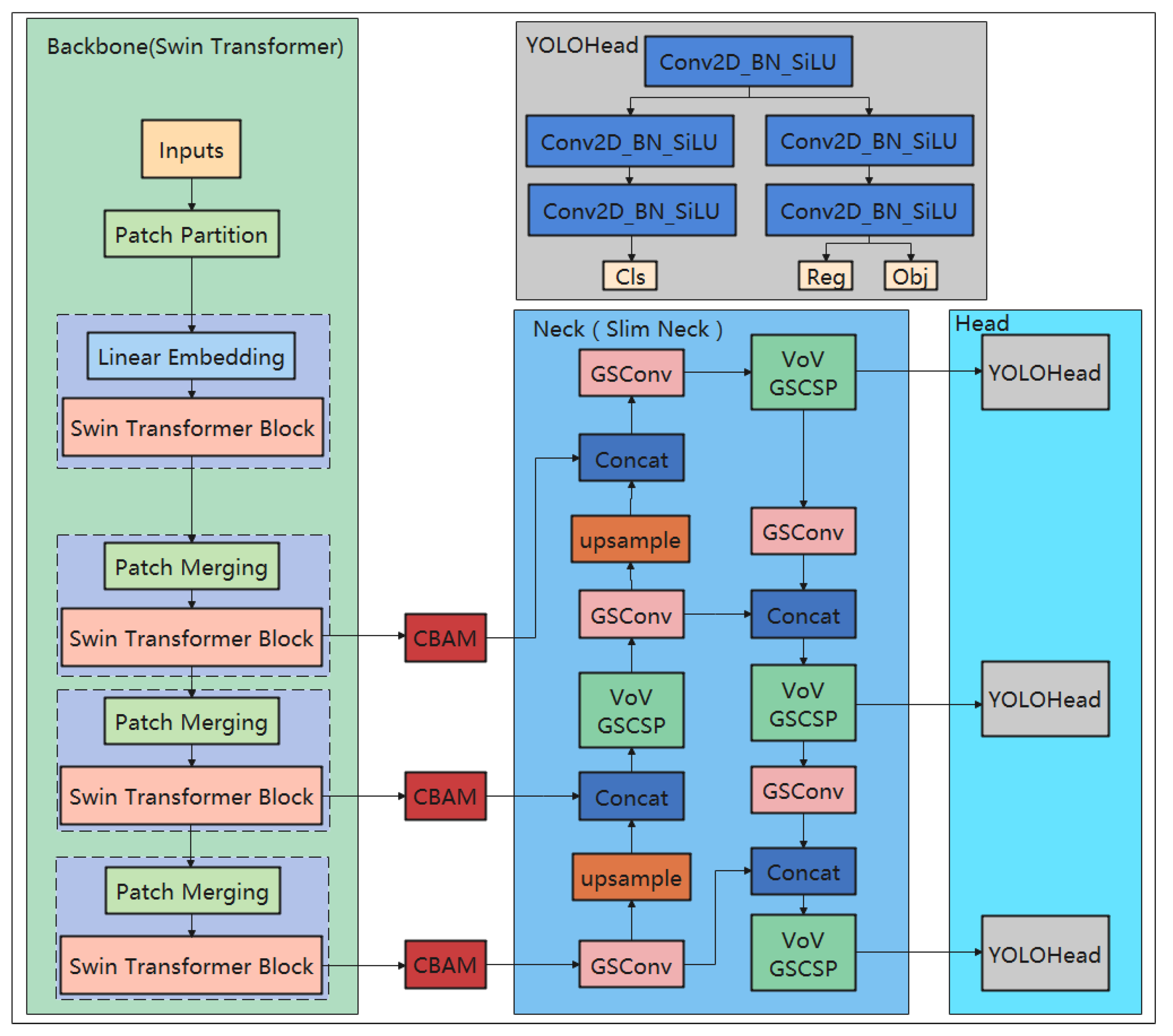
(1) The backbone network CSPDarknet of the YOLOX network is replaced with Swin Transformer architecture, and the convergence speed and detection accuracy are improved compared with the training results of the original YOLOX algorithm on the same flame smoke data.
(2) Add CBAM attention mechanism after the three effective output networks of the backbone network to make the network pay more attention to the target to be detected, improve the detection effect, and solve the situation of easy error and omission detection in the context of a complex environment.
(3) The PANet network model in the Neck part of the original YOLOX algorithm is replaced by the Slim Neck network model, which still keeps the model with sufficient accuracy while reducing the computational effort and network complexity.

2. Materials and Methods

2.1. YOLOX Target Detection Algorithms

The BaseDetection group of Megvii Technology Limited Research Institute introduced the YOLOX algorithm in 2021 as the most recent iteration of the YOLO series of target algorithms, fusing cutting-edge academic findings with the demands of engineering practice [9]. As a starting point: YOLOX employs YOLOv3 and Darknet53; it adopts the structural design and SPP layer of Darknet53; it includes EMA weight update, consine lr_schedule, IoU loss, and IoU-aware branch; it uses BCE loss to train cls and obj, and it uses IoU loss as the test branch. Only RandomHorizontalFlip, ColorJitter, multi-scale, and mosaic are used for data enhancement without employing the Imagenet pre-training approach because RandomResizedCrop and mosaic enhancement overlap. The following improvements are primarily made by the YOLOX algorithm: the YOLOX algorithm separates the decoupling heads, separately implements classification and regression [10,11], and only combines them in the final prediction because the YOLO family of algorithms uses combined decoupling heads and simultaneous implementation of both classification and regression, which can hinder the network’s ability to recognize the target. Second, YOLOX does not employ a priori frames, which decreases the number of parameters by around two-thirds and simplifies the training and decoding stages, increasing the speed and effectiveness of operations. Its overall structure is shown in Figure 1.

2.2. Model Improvements and Optimization

The primary feature extraction network used by YOLOX is CSPDarknet, which consists of numerous Cross Stage Partial (CSP) layers with numerous residual networks. The CSP layer connects the input features with little processing directly to the output features of numerous residuals with significant residual edges. Even though this method successfully addresses the gradient disappearance issue brought on by deepening the network, the residual will still transmit feature information along with the contained noise to the deeper network, which will negatively impact the backbone network’s ability to extract features.
Smaller flames and thinner smoke are characteristics of early-stage fires. In an experimental study, it was discovered that the YOLOX algorithm had poor flame and smoke detection accuracy, inaccurate location detection, and delayed flame and smoke detection at the initial occurrence of a laboratory fire. Thus, the backbone network CSPDarknet of YOLOX is replaced in this study with Swin Transformer, and the Convolutional Block Attention Module (CBAM) is added after each of the three useful feature layers extracted from the backbone network, in order to address these flaws of YOLOX in flame and smoke detection. The Slim Neck model takes the place of the PANet model in the Neck section of the original YOLOX algorithm, effectively reducing computational effort and network complexity while maintaining enough accuracy. The enhanced YOLOX network’s structural diagram is depicted in Figure 2 below.

2.3. Swin Transformer

The original YOLOX model’s early-fire targets are little flames, making the model easy to overlook. The improved YOLOX model makes up for the original YOLOX network’s lack of long-distance modeling and its inability to obtain global information by using Swin Transformer as its backbone network to enhance its ability to extract feature information of flame targets. This also improves the model’s detection effect on little flames.
Convolutional neural network-based deep learning methods now in use offer the advantages of high accuracy, low costs, and fast speeds, but they fall short of Transformer in terms of processing the link between visual elements and objects [12,13,14]. Transformer is a deep neural network that was initially used in the field of natural language processing and is based on a self-attentive mechanism (NLP). Researchers have recently suggested numerous approaches to employ the Transformer to conduct computer vision tasks with good results, even outperforming convolutional neural networks, as a result of its potent performance. By breaking up photos into many image blocks for processing, Vision Transformer (Vit) proved, for the first time, that the Transformer design can also be directly applied to images [15]. Transformer was successfully used for the target detection problem by DETR as the first method [16]. DETR utilizes the set matching loss function and adds a Transformer encoder and decoder to a common CNN model (As ResNet-50/101). A sliding window attention mechanism is proposed by Swin Transformer to compute self-attention within a window region without overlap, modeling only local relationships at each layer, while being able to continuously reduce the feature map width and height, and expand the perceptual field [17]. Swin Transformer introduces the hierarchical construction method typically used in CNN to build hierarchical transformers. Compared to ViT, the computational complexity of Swin Transformer is substantially reduced.
The use of Transformer in computer vision has two fundamental difficulties. First, the visual target is constantly changing, and the performance of the visual Transformer may not be very effective in various circumstances. Second, Transformer’s calculation based on global self-attentiveness will require a significant amount of processing if the image quality is high and there are numerous pixel points. Swin Transformer suggests a strategy to create the Transformer in a hierarchical approach by incorporating sliding window operations in order to address these two problems. By limiting the attentional computation to a window, the sliding window operation can introduce local awareness of CNN convolutional procedures while also reducing computing cost. The network’s computing effort is drastically reduced by Swin Transformer’s method of maintaining the computational region in windowed units, which reduces complexity to a linear scale of image size.
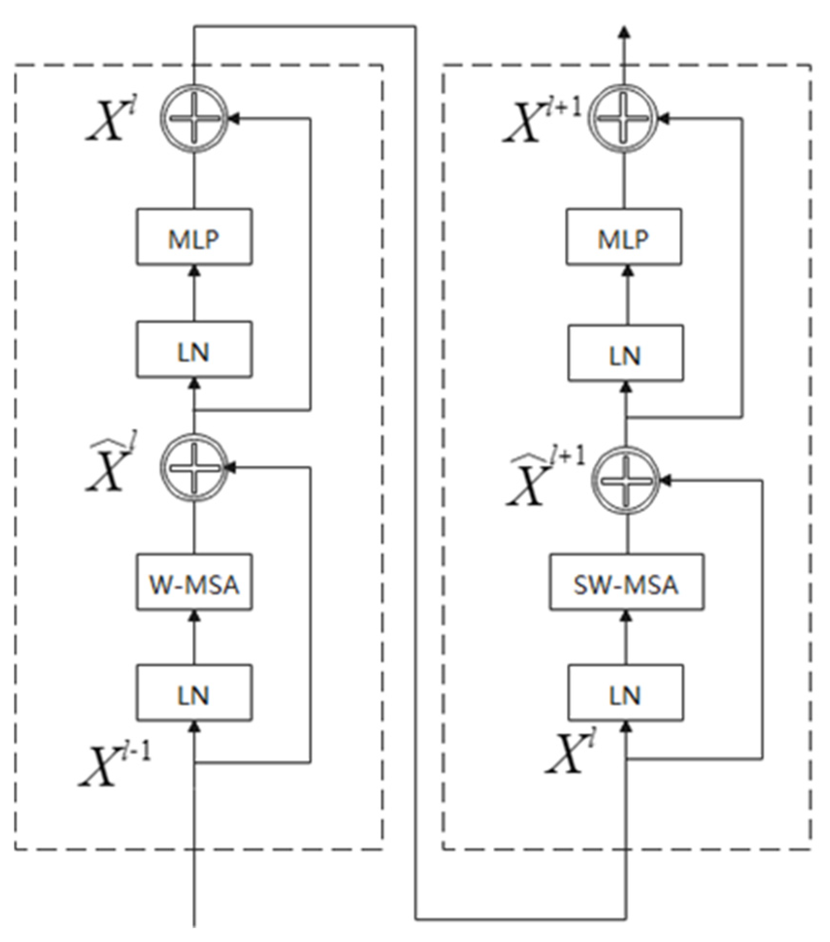
Swin Transformer consists of the following main components: MLP (Multi-layer Perceptron), W-MAS (Window Multi-head Self Attention), SWMSA (Shifted Window based Multi-head Selfattention), and LN (Layer Normal-ization). Its backbone network is shown in Figure 3.
The input features to the Swin Transformer backbone network are shown in Figure 3 to first pass through the normalization layer for normalization, the windowed multi-headed self-attentive layer for feature learning, the residuals are computed, the multilayer perceptron through the normalization layer, and, finally, another residual operation to obtain the output features of this layer. The construction of the sliding window multi-head self-attentive layer is comparable to that of the window multi-head self-attentive layer, with the exception that the sliding window action is necessary for the sliding window multi-head self-attentive layer’s computational feature portion. After the backbone network process, the output of each component is expressed as shown in Equations (1)–(4).
X ^ l = W   -   MSA ( LN ( X l 1 ) ) + X 1
X l = MLP ( LN ( X ^ l ) ) + X ^ l
X ^ l + 1 = SW-MSA ( LN ( X l ) ) + X l
X l + 1 = MLP ( LN ( X ^ l + 1 ) ) + X ^ l + 1
where X ^ l and X l denote the output features of the (S)W-MSA module and the MLP module for block l , respectively; W-MSA and SW-MSA denote window-based multi-head self-attention using regular and shifted window partitioning configurations, respectively.
Figure 4 depicts the total network architecture of the Swin Transformer. The input feature map is passed through a PatchPartition layer as the network develops, changing the smallest unit of the image from a pixel to a patch, with each patch being treated as a token, and the result is a three-dimensional matrix of H/4 × W/4. The downsampling, resolution, channel number, and hierarchy are all controlled by the patch merging layer. Each set of 2 × 2 patches’ features is joined together by the first patch merging layer, which also connects a linear layer to the spliced features. These features are then processed by the Swin Transformer backbone structure. The output dimension is set to C and the number of tokens is maintained at H/4 × W/4 in the process of “stage1”. Then, in “stage2”, the output dimension is set to 2C and the number of tokens is decreased by a factor of 4 times to H/8 × W/8. After changing the output dimension to 2C, feature processing is carried out. Each stage, which is repeated six times and twice, denotes a level. “stage2” and “stage1” are repeated twice; “stage3” and “stage4” are similar to the previous stages, and the output is H/16 × W/16 and H/32 × W/32, respectively, and the output dimension is 4C and 8C, repeated 6 times and 2 times, respectively. Each stage represents a level. Similar to common convolutional neural networks like ResNet [18], this is a hierarchical structure. This makes it simple to adapt Swin Transformer’s architecture to use the backbone network for various vision tasks.
The self-attentive mechanism is the key module of Transformer, which is calculated as shown in Equation (5). Where Q, K, and V are query, key, and value, respectively, and d is the number of query dimensions.
A = Attention ( Q , K , V ) = SoftMax ( Q K T / d ) V
Traditional Transformer structures typically use global self-attention to compute the relationship between one token and all other tokens, but because of the complexity increase caused by the global computation, they are unsuitable for vision problems that call for intensive prediction or the representation of high-resolution images with numerous token sets. Swin Transformer suggests computing self-attention within a local window for effective modeling. The windows are set up so that the photos are consistently segmented and without overlap. The window based on hxw patches has a much lower computational complexity than the window based on global attention.

2.4. CBAM Attention Mechanism

To solve the issue of the complicated backdrop of the laboratory setting and the target detection model being subject to interference from the background environment when identifying targets, the CBAM attention mechanism is used to help the model concentrate on crucial details while suppressing unimportant ones. This improves the feature reinforcement of deep-level targets and makes it possible for the model to more precisely extract flame and smoke target features, improving target detection precision.
Woo et al. [19] suggested the CBAM (Convolutional Black Attention Module) module as an attention module. To give the extracted features a better ability to represent data, CBAM will process the input feature layers in the Channel Attention Module (CAM) and Spatial Attention Module (SAM), respectively. Figure 5 presents an illustration of the structure.

2.4.1. Channel Attention Mechanism

The two feature layers of size CxHxW are obtained by average pooling and maximum pooling, respectively. They then pass through two MLP (Multilayer Perceptron) neural networks, the first of which has the number of neurons C/r and the activation function ReLU, and the second of which has the number of neurons C. The channel attention mechanism focuses on the meaningful information in the input image. The two results are added, then each channel’s weight value in the input feature layer is obtained by passing them through a Sigmoid function, where C is the number of channels in the input feature layer and r is the descent rate. The obtained weight value is then multiplied by the original input feature layer to produce the new feature. Equation (6) illustrates the feature obtained for an input feature following the channel attention process (6).
F = M C ( F ) F
where F is the input’s feature matrix, F’ is the channel attention mechanism’s output feature mapping, Mc is the channel’s compression weight matrix, and ⊗ is the matrix elements sequentially multiplied. In Figure 6, the structure diagram is displayed.

2.4.2. Spatial Attention

The spatial attention mechanism focuses on the target’s location information, and the channel attention mechanism outputs feature layers that are subjected to maximum pooling and average pooling to produce two stacked feature layers of size 1 × H × W. Next, the weight values are obtained using a 7 × 7 convolution operation with a channel number of 1, a Sigmoid function, and the input feature layers, and the weight values are then multiplied by the input feature layers to produce the final result. Equation (7) illustrates the feature F” acquired following the spatial attention mechanism for the output feature F’ of the channel attention mechanism (7).
F = M S ( F ) F
where F″ denotes the feature matrix of the output of the spatial attention mechanism; Ms is the spatial compression weight matrix. The structure diagram is shown in Figure 7.

2.5. Slim Neck Module

Accuracy and speed are equally crucial for the identification of flame and smoke at a fire scene. The following suppression of the fire will be more challenging if poor detection results in delayed notice. The model’s complexity is decreased while maintaining accuracy and speed by using the Slim Neck method.
The detection phase currently uses single-stage and two-stage deep-learning-based target detection methods. Due to the idea of sparse detection, two-stage detectors perform better at identifying small objects and can increase mean accuracy (mAP), but at the expense of speed. Although single-stage detectors are faster than two-stage detectors in terms of speed, which is crucial for industry, they are less effective than two-stage detectors at detecting and localizing small items.
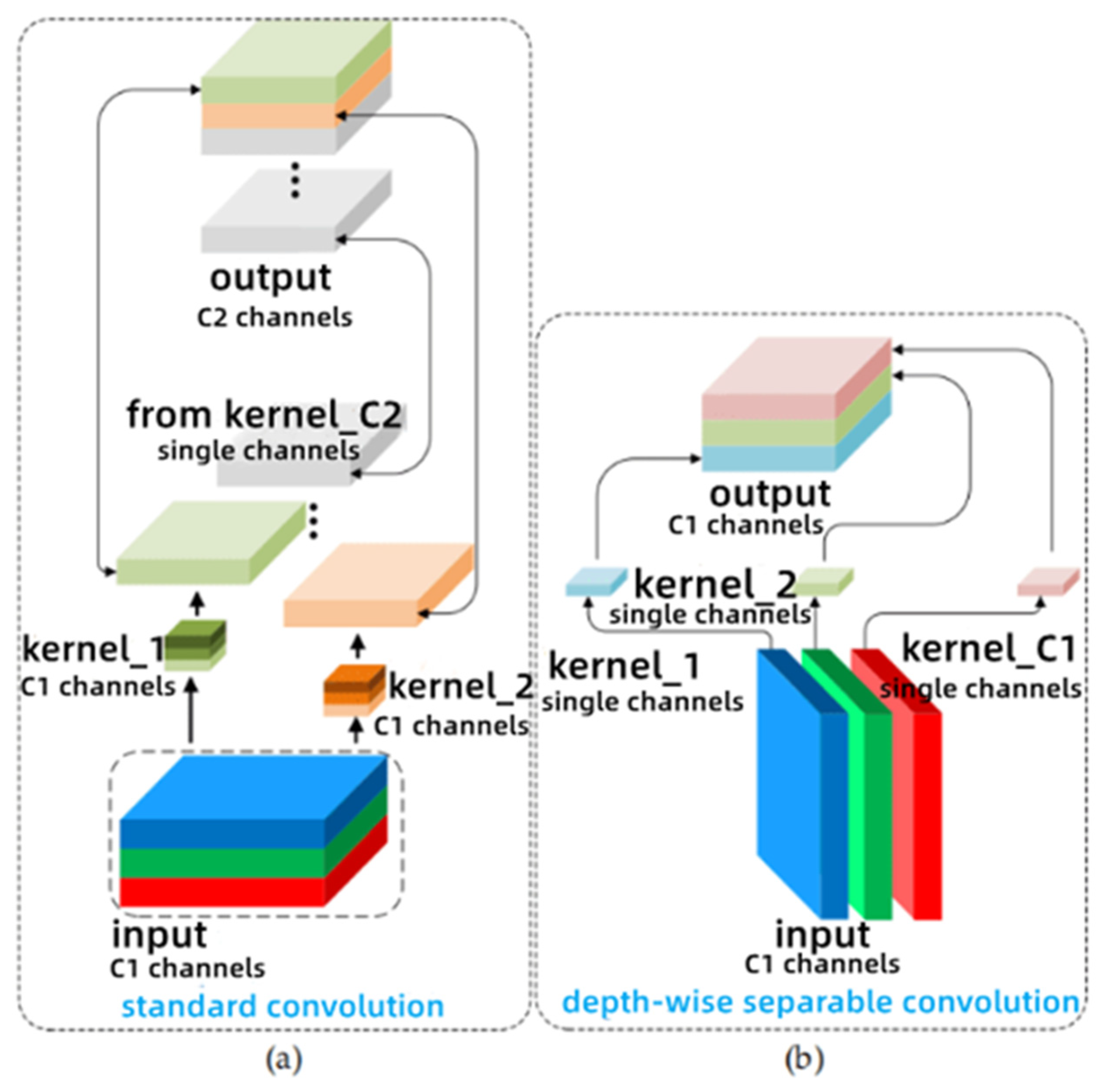
According to the conventional wisdom in brain-like research, a model’s nonlinear representational power increases with the number of neurons it contains. A powerful model cannot be created by simply indefinitely increasing the number of model parameters because biological brains have a much greater capacity for information processing and consume less energy than computers [20,21]. Many outstanding lightweight works, like Xception, MobileNets, and ShuffleNets, use Depth-wise Separable Convolution (DSC) operations to cut down on the number of parameters and FLOPs, which helps to offset the high computational cost at this point. Although the speed of the detector is substantially increased by the DSC operation, the negative of DSC is that the channel information of the input image is split during the computation. As a result, the accuracy of these models is poorer when they are used for detection.
However, the drawbacks of DSC are directly amplified in the backbone, whether for image classification or detection, and this shortcoming results in a much lower feature extraction and fusion capability of DSC than SC. This is because many lightweight models design the basic architecture of a deep neural network using DSC-only thinking. The feature maps created by channel rearranging the output channels of DSC alone are still “deeply separated” when SC and DSC are combined. Figure 8a,b depicts how DSC and Standard Convolution were calculated (SC).
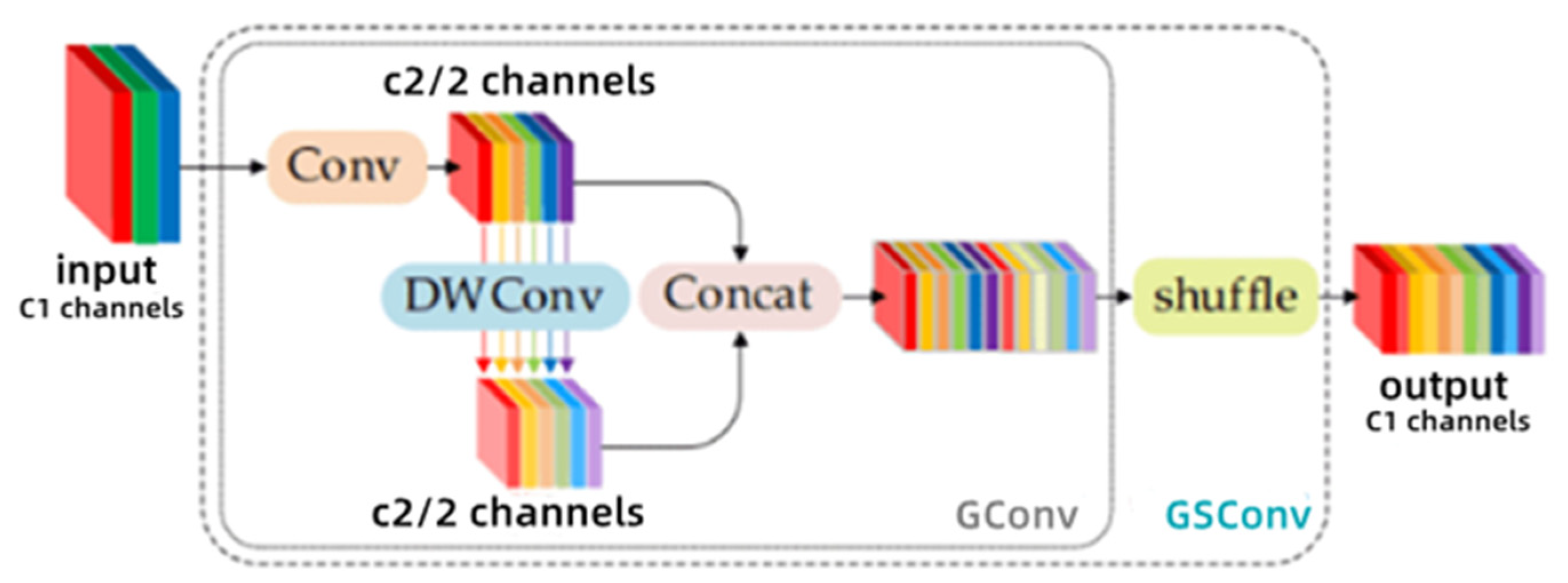
An entirely new technique, GSConv, was developed to bring the output of DSC as near to SC as possible. As seen in Figure 9, the information produced by SC is shuffled into every component of the information produced by DSC. With this method, the DSC output can incorporate all of the data from the SC.
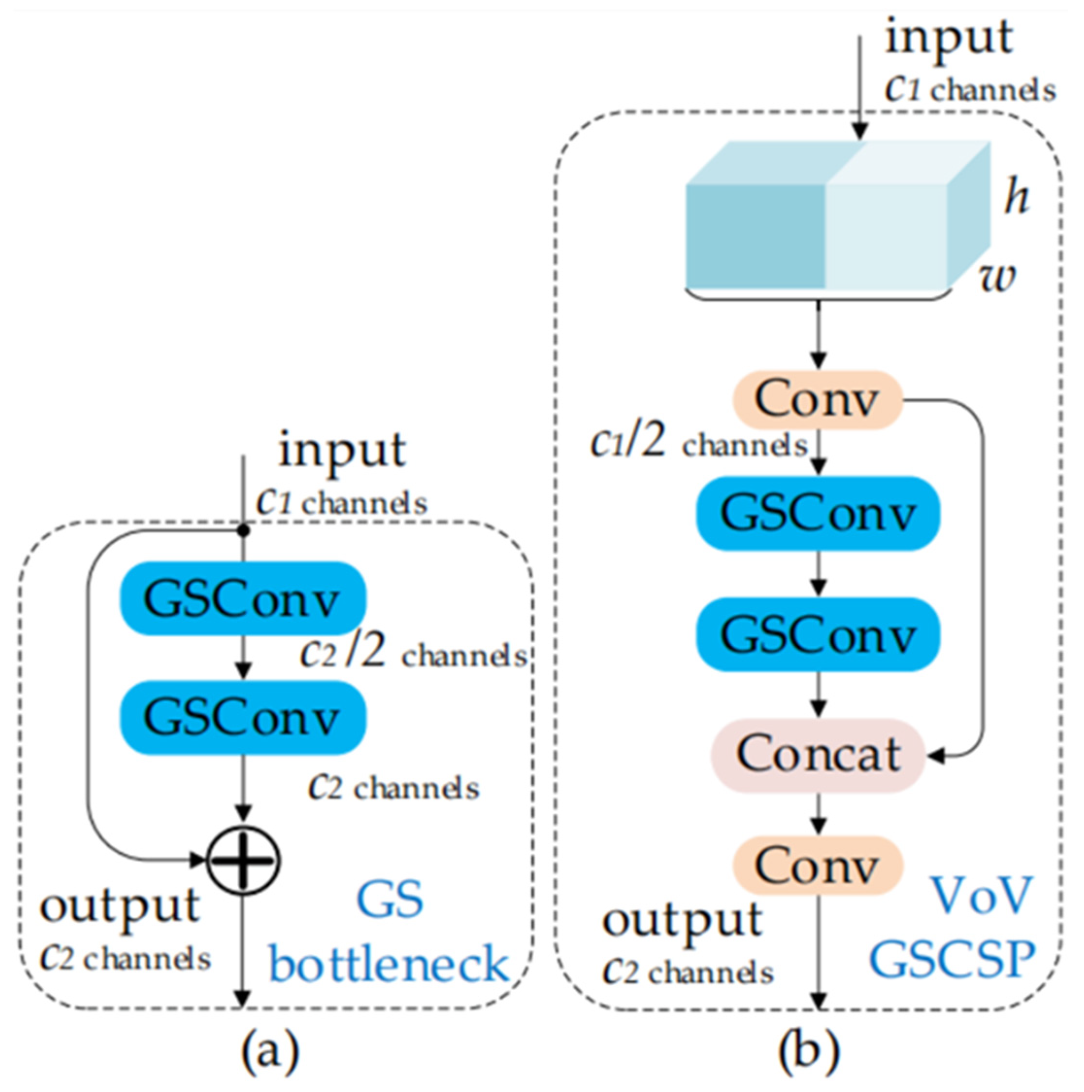
The Slim Neck structure is then created based on the theory behind these techniques by researching general techniques to improve CNN learning, such as DensNet, VoVNet, and CSPNet. First, the lightweight convolutional approach GSConv was employed in place of SC to simplify the model while maintaining accuracy. Slim Neck, a feature of GSConv that better balances speed and accuracy [22], has a computational cost that is roughly 60–70% lower than SC. The cross-level partial network module VoV-GSCSP is designed using a one-time aggregation method, continuing the introduction of the GSbottleneck based on GSConv, which not only lowers the complexity of computation and network structure but also maintains appropriate accuracy. Figure 10a illustrates the Gsbottleneck module structure and Figure 10b shows the VoV-GSCSP structure.

2.6. Experimental Platform

The platform for this paper was a desktop computer running Windows 10 64-bit, with an Intel i9-12900KF processor clocked at 3.9 GHz, an NVIDIA GeForce GTX3090Ti graphics card, 32GB of RAM, PyTorch version 1.11.0, and CUDA version 11.3.0. The testing environment was the same as the training set.

2.7. Network Training

5000 images, including 3046 flame targets and 2532 smoke targets, made up the training dataset for the network in the study. These images were randomly split into the training set, validation set, and test set in the ratio of 8:1:1, and the division results are displayed in Table 1. Stochastic Gradient Descent (SGD) and linear scaling (lrxBatch-Size/64) of the learning rate were used during the training process. The training was carried out utilizing the weights trained by themselves as pre-training weights for 300 epochs training. The first 50 rounds of training were freeze training with batch size set to 16, and the following training was thaw training with batch size set to 8.

2.8. Model Evaluation Indicators

The average precision AP (Average Precision), the summed mean F1 value (F1-score), the accuracy P (Precision), the recall R (Recall), and the average AP value mAP (Mean Average Precision) are used to assess the trained model. AP, F1, Precision, Recall, and mAP are among them and are calculated as indicated in (8) to (12).
AP = 0 1 d r Precision × Recall
F 1 = 2 × Precision × Recall Precision + Recall
Precision = TP TP + FP × 100 %
Recall = TP TP + FN × 100 %
mAP = 1 N i = 0 N 1 AP i
In Equation (10), TP (True Positive) is the number of correctly segmented positive samples; FP (False Positive) is the number of incorrectly segmented positive samples; and FN (False Negative) is the number of incorrectly segmented negative samples. In Equation (8), r is the integral variable, which is the integral of the re-call-precision product; AP is the area bounded by the coordinate axis and the PR (Precision-Recall) curve, and the value ranges from 0 to 1. Since there are 2 classes in this study, N = 2, and APi is the AP value corresponding to 2 classes of detection targets; N in Equation (12) denotes N classes of detection targets.

3. Results

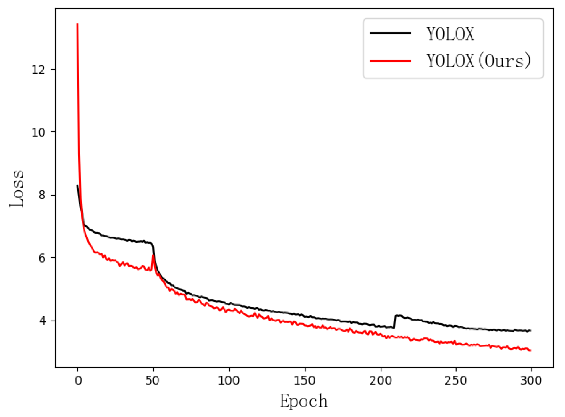
The learned loss function values are displayed in Figure 11 for the network topology in Figure 2, which was trained on the training set. Based on the identical pre-trained model (data for pre-trained models from a portion of COCO2017), the findings reveal that the enhanced YOLOX in this study converges more quickly, and the final loss value is smaller and more stable, at roughly 2.7. The final Loss values of different improvement methods are shown in Table 2.

3.1. Ablation Experiments

To examine the effects of various network branches on the overall model, ablation experiments are a popular experimental technique in the field of deep learning [23]. Three elements of the YOLOX model are improved in this study, and, to analyze the effects of each improvement portion on the model performance, seven sets of ablation experiments are created to examine the effects of various model modifications. In Table 3, “✓“ indicates that the enhancement was employed, while “×” indicates that it was not. All trials were trained on the dataset created in this paper using identical parameters and environments. mAP is the data obtained from the test set.
Analysis of the data in the table reveals that Improvement 1 uses the Swin Transformer network structure as the Backbone of the YOLOX model and that the mAP is improved by 4.35% in comparison to the original YOLOX model, demonstrating that the Swin Transformer has superior feature extraction ability to the CSPDarknet. With a mPA improvement of 0.96%, Improvement 4 enhances Improvement 1 by adding the CBAM attention mechanism module beneath the three efficient feature extraction layers. This allows the network to concentrate more on crucial features and suppress unnecessary ones. Improvement 7 improves the mAP by 0.78% by replacing the PAnet network in the Neck section with the Slim Neck network, which is based on Improvement 4. This minimizes the complexity of the computation and network structure. Comparing the final improvement algorithm to the initial YOLOX algorithm, mAP is improved by 6.09%.

3.2. Analysis of Test Results of Different Models

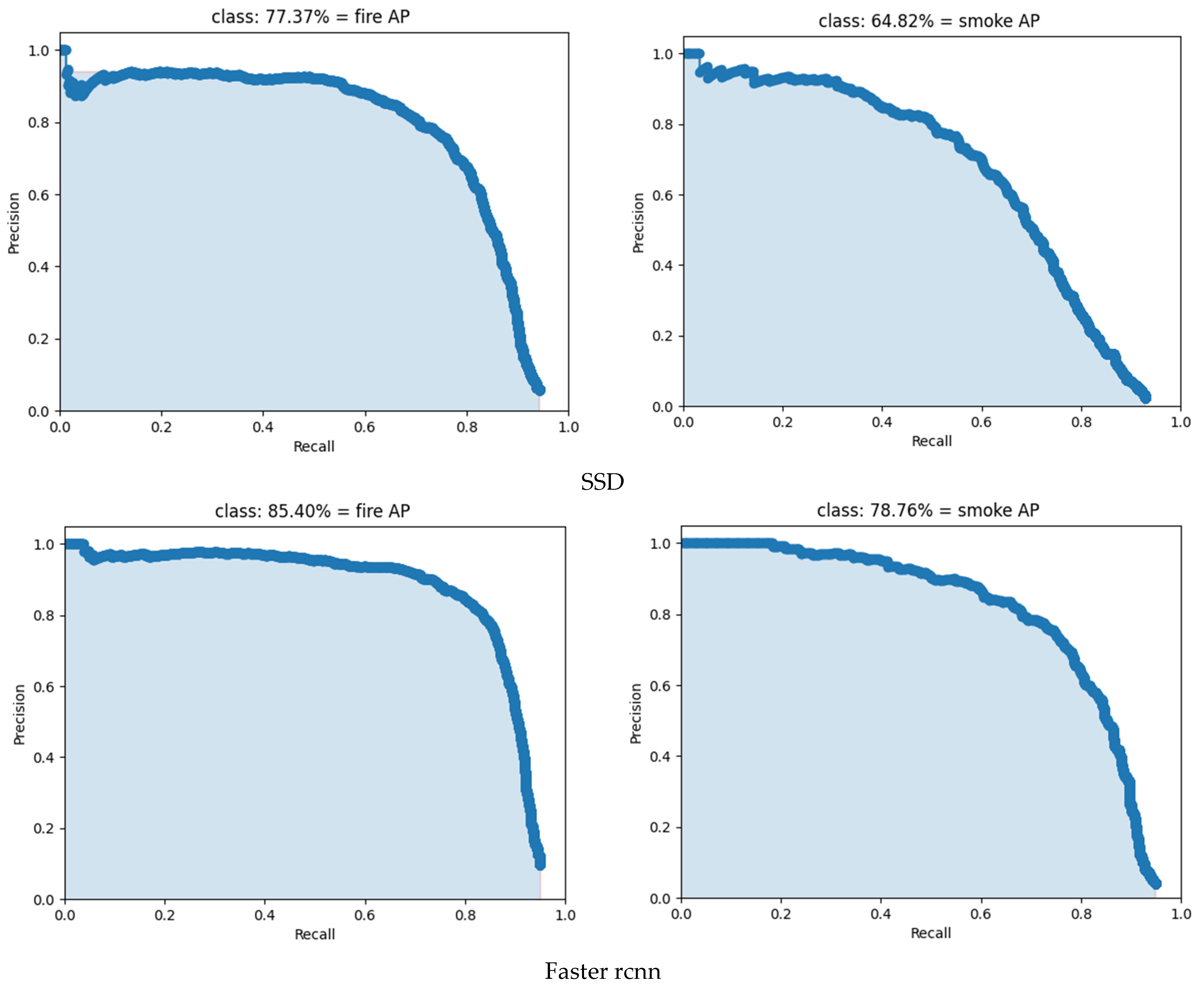
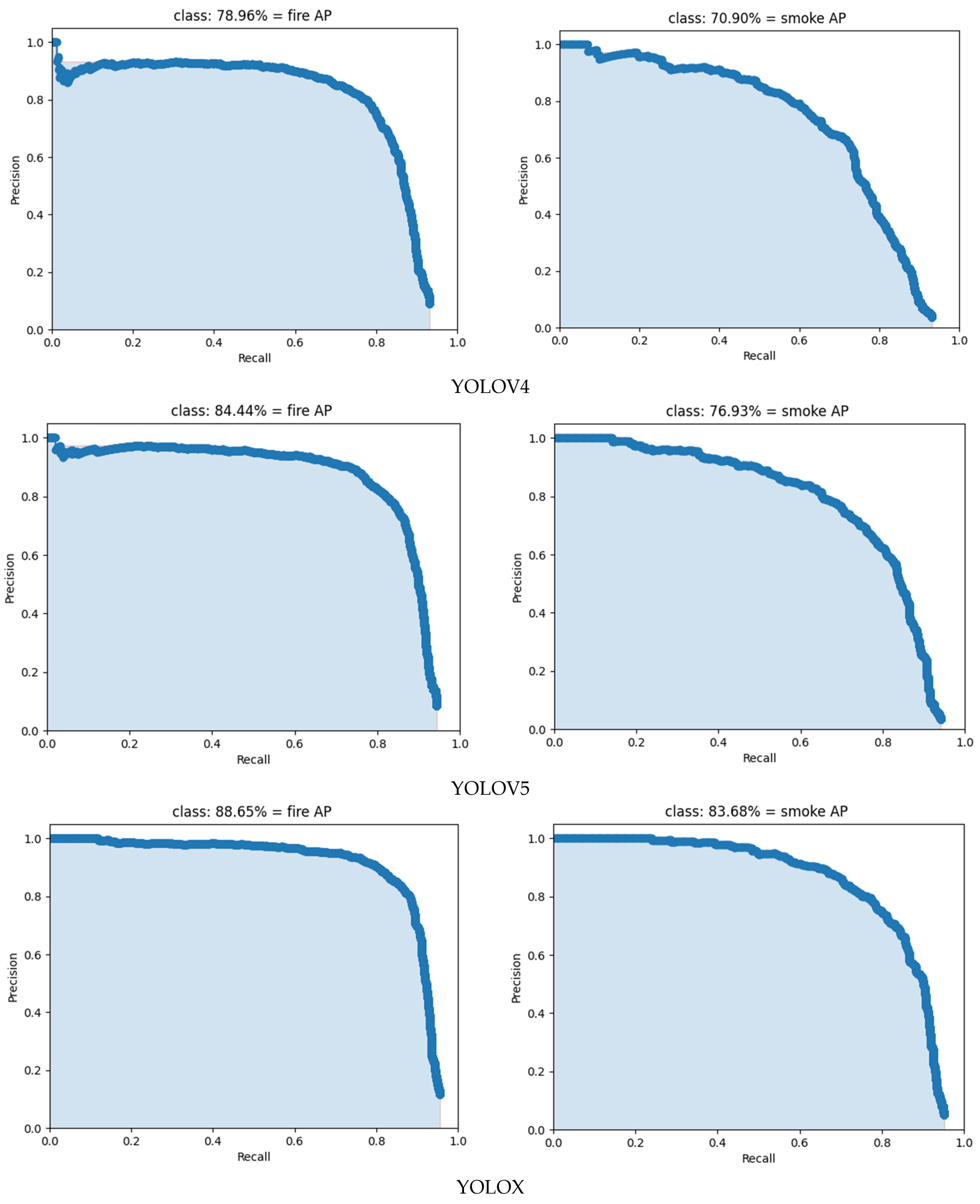
The improved YOLOX model was compared to five other models on the same dataset used in this paper to assess how well it performed at detecting flames and smoke. The evaluation indices of all the algorithms were totaled, and the results of the comparison experiments are shown in Table 4 and Figure 12 (PR curves for flame and smoke, respectively).
When compared to the original YOLOX model, SSD model, Faster R-CNN model, YOLOv4 model, and YOLOv5 model, the revised YOLOX model has varying degrees of performance improvement, according to the results in Table 3 and Figure 12. The upgraded YOLOX model exhibits mAP improvements of 21.17% compared to SSD, 10.08% compared to Faster R-CNN, 17.33% compared to YOLOv4, 11.58% compared to YOLOv5, and 6.09% compared to the original YOLOX, showing that the improved YOLOX utilizing three different techniques has superior performance. In terms of accuracy and recall, the F1 score can address the issue of a one-sided evaluation of the model and allow for a more thorough review. The flame F1 score of the enhanced YOLOX model is 89%, while the smoke F1 score is 87%, with the improved YOLOX model scoring 26%, 13%, and 20% higher than the other five models, respectively. It can be said that the upgraded YOLOX model performs better overall and recognizes flame and smoke images more accurately.

3.3. Model Detection Effect

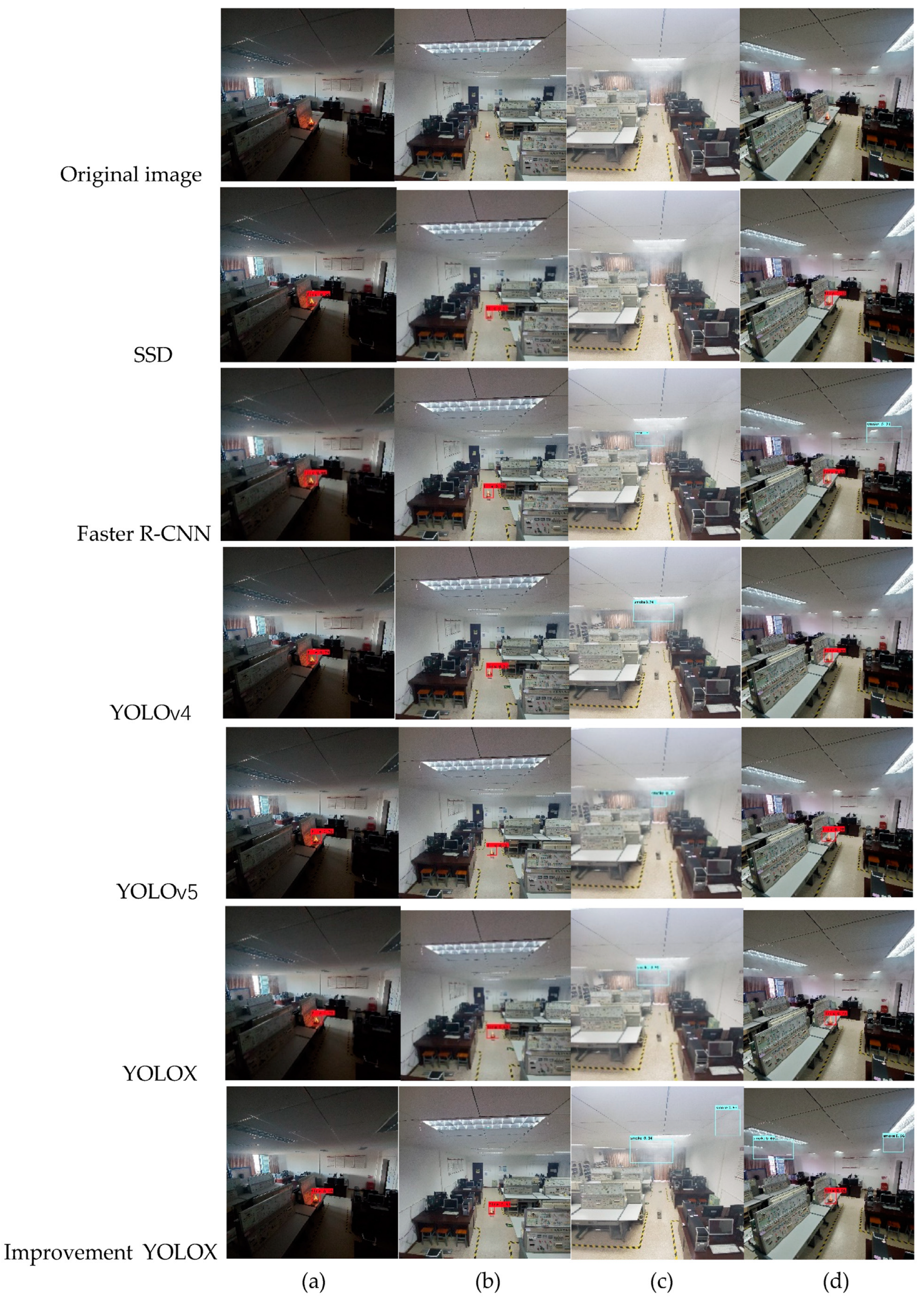
To further verify the advantages of the improved YOLOX algorithm over other algorithms in this paper, the detection results of several models for flame and smoke images in a fire are listed, as shown in Figure 13. Figure 13a shows the case where the flame is more obvious and smoke is not obvious in a darker environment; Figure 13b shows the case where the smoke is more obvious and the flame is not obvious in a brighter environment; Figure 13c shows the case where there is no flame and smoke is more obvious in a brighter environment; and Figure 13d shows the case where both flame and smoke are obvious in a brighter environment. The detection text box has the name of the predicted target and the confidence level above it, and the higher confidence level indicates the better performance of the algorithm. As can be seen from the figure, compared with the other five algorithms, the improved YOLOX algorithm has more accurate position detection and a higher confidence level for flame and smoke, which is more suitable for flame and smoke detection in laboratory fires.

4. Discussion

The enhanced YOLOX model is the most effective for recognizing flames and smoke among the trained and validated models. The size of the upgraded YOLOX model is greater than previous algorithm models, and it takes longer to train the model. Additionally, it is easy for memory overload to occur during training. So that the model may be trained smoothly, the values of BatchSize and free BatchSize should be appropriately adjusted in accordance with the amount of GPU memory. We can suitably expand the data set using flip, rotation, scale, and other techniques if we wish to further improve the mAP of flames and smoke detection.

5. Conclusions

For small fire targets and smoke targets in laboratory fire detection, the original YOLOX algorithm has low detection accuracy and imprecise detection location. The improved YOLOX model uses Swin Transformer as the YOLOX backbone network. The features of the Swin Transformer network are learned by moving the window; moving the window not only brings greater efficiency, since the self-attention is calculated within the window, but it also greatly reduces the length of the sequence. Shifting (moving) the operation makes the two adjacent windows interact with each other, so that there is a cross-window connection between the upper and lower layers, thus disguising the ability to achieve global modeling, enhancing its ability to extract information about the flame target features, making up for the lack of long-distance modeling of the original YOLOX network, which has no ability to obtain global information, and enhancing the model’s effectiveness in detecting small flames. The CBAM attention mechanism is also introduced to enable the model to focus on important features and suppress unnecessary features in the complex background of the laboratory, which helps to enhance the feature reinforcement of deep-level targets and enables the model to extract flame and smoke target features more accurately, thus enhancing the accuracy of target detection. The introduction of the Slim Neck method in the Neck part can reduce the complexity of the model and maintain accuracy and speed. After experimental validation, it was proved that the improved algorithm has more accurate position detection and higher confidence for flame and smoke, and the mAP is improved by 6.09%, 21.17%, 10.08%, 17.33%, and 11.58% compared with the original YOLOX, SSD, Faster R-CNN, YOLOv4, and YOLOv5 algorithms, respectively.
In the subsequent work, we will mostly focus on determining how to branch and lighten the model without sacrificing accuracy, deploy the model to mobile or embedded devices, and increase the study’s applicability within various kinds of laboratories.

Author Contributions

Conceptualization, M.L.; Methodology, M.L. and L.X.; Software, M.L. and M.C.; Supervision, Y.Y.; Visualization, J.Y.; Writing—review and editing, M.L. All authors have read and agreed to the published version of the manuscript.

Funding

This study was supported by the Qianjiaohe KY word [2021] 012 Major Research Project of Innovative Groups in Guizhou Provinceand the 2019 Guizhou Provincial Undergraduate Teaching Project (209010).

Institutional Review Board Statement

Not applicable.

Informed Consent Statement

Not applicable.

Data Availability Statement

Not applicable.

Conflicts of Interest

The authors declare no conflict of interest.

References

  1. Zhao, D.; Meng, K.; Jiang, N.; Li, T.; Liu, S. Analysis of the construction of laboratory safety management system in universities based on information platform. China Insp. Test. 2019, 27, 49–50. [Google Scholar]
  2. Wu, F. Research and Implementation of Fire Detection Algorithm Based on Deep Learning; Hangzhou University of Electronic Science and Technology: Hangzhou, China, 2020. [Google Scholar]
  3. Li, X.; Zhang, D.; Sun, L. A CNN-based lightweight flame detection method for complex scenes. Pattern Recognit. Artif. Intell. 2021, 34, 415–422. [Google Scholar]
  4. Luo, Z. UAV-Based Forest Fire Monitoring and Path Planning Research; Xi’an University of Technology: Xi’an, China, 2021. [Google Scholar]
  5. Tang, D. Research on Deep Learning Method for Forest Fire Detection; Xi’an University of Technology: Xi’an, China, 2021. [Google Scholar]
  6. Ma, S. Research on Video-Based Fire Detection Method for Cruise Ships; Jiangsu University of Science and Technology: Zhenjiang, China, 2021. [Google Scholar]
  7. Wang, L.; Zhao, H. Improving YOLOv3 for fire detection. Comput. Syst. Appl. 2022, 31, 143–153. [Google Scholar]
  8. Yu, L.; Liu, J. Flame image recognition algorithm based on improved Mask R-CNN. Comput. Eng. Appl. 2020, 56, 194–198. [Google Scholar]
  9. Ge, Z.; Liu, S.; Wang, F.; Sun, J. YOLOX: Exceeding YOLO series in 2021. arXiv 2021, arXiv:2107.08430. [Google Scholar]
  10. Ali, M.R.; Ma, W. New exact solutions of Bratu Gelfand model in two dimensions using Lie symmetry analysis. Chin. J. Phys. 2020, 65, 198–206. [Google Scholar] [CrossRef]
  11. Ayub, A.; Sabir, Z.; Altamirano, G.C.; Sadat, R.; Ali, M. RCharacteristics of melting heat transport of blood with time-dependent cross-nanofluid model using Keller–Box and BVP4C method. Eng. Comput. 2022, 38, 3705–3719. [Google Scholar] [CrossRef]
  12. Lin, T.Y.; Dollár, P.; Girshick, R.; He, K.; Hariharan, B.; Belongie, S. Feature pyramid networks for object detection. In Proceedings of the IEEE Conference on Computer Vision and Pattern Recognition, Honolulu, Hawaii, 21–26 July 2017; pp. 2117–2125. [Google Scholar]
  13. Singh, B.; Davis, L.S. An analysis of scale invariance in object detection-SNIP. In Proceedings of the IEEE Conference on Computer Vision and Pattern Recognition, Salt Lake City, UT, USA, 18–23 June 2018; pp. 3578–3587. [Google Scholar]
  14. Singh, B.; Najibi, M.; Davis, L.S. Sniper: Efficient multi-scale training. Adv. Neural Inf. Process. Syst. 2018. [Google Scholar] [CrossRef]
  15. Dosovitskiy, A.; Beyer, L.; Kolesnikov, A.; Weissenborn, D.; Zhai, X.; Unterthiner, T.; Dehghani, M.; Minderer, M.; Heigold, G.; Gelly, S.; et al. An Image is Worth 16x16 Words: Transformers for Image Recognition at Scale. arXiv 2020. [Google Scholar] [CrossRef]
  16. Carion, N.; Massa, F.; Synnaeve, G.; Usunier, N.; Kirillov, A.; Zagoruyko, S. End-to-end object detection with transformers. In European Conference on Computer Vision; Springer: Cham, Switzerland, 2020; pp. 213–229. [Google Scholar]
  17. Liu, Z.; Lin, Y.T.; Cao, Y.; Hu, H.; Wei, Y.; Zhang, Z.; Lin, S.; Guo, B. Swin transformer: Hierarchical vision transformer using shifted windows. In Proceedings of the IEEE/CVF International Conference on Computer Vision, Montreal, QC, Canada, 10–17 October 2021; pp. 10012–10022. [Google Scholar]
  18. He, K.M.; Zhang, X.Y.; Ren, S.Q.; Sun, J. Deep residual learning for image recognition. In Proceedings of the IEEE Conference on Computer Vision and Pattern Recognition, Las Vegas, NV, USA, 27–30 June 2016; pp. 770–778. [Google Scholar]
  19. Woo, S.; Park, L.; Lee, J.Y.; Kweon, I.S. CBAM: Convolutional block attention module. arXiv 2018, arXiv:1807.06521. [Google Scholar]
  20. Ali, M.R. The Method of Lines Analysis of Heat Transfer of Ostwald-de Waele Fluid Generated by a Non-uniform Rotating Disk with a Variable Thickness. J. Appl. Comput. Mech. 2021, 7, 432–441. [Google Scholar] [CrossRef]
  21. Mousa, M.M.; Ali, M.R.; Ma, W. A combined method for simulating MHD convection in square cavities through localized heating by method of line and penalty-artificial compressibility. J. Taibah Univ. Sci. 2021, 15, 208–217. [Google Scholar] [CrossRef]
  22. Li, H.; Li, J.; Wei, H.; Liu, Z.; Zhan, Z.; Ren, Q. Slim-neck by GSConv: A better design paradigm of detector architectures for autonomous vehicles. arXiv 2022, arXiv:2206.02424. [Google Scholar]
  23. Ren, S.; He, K.; Girshick, R.; Sun, J. Faster R-CNN: Towards real-time object detection with region proposal networks. IEEE Trans. Pattern Anal. Mach. Intell. 2017, 39, 1137–1149. [Google Scholar] [CrossRef] [PubMed] [Green Version]
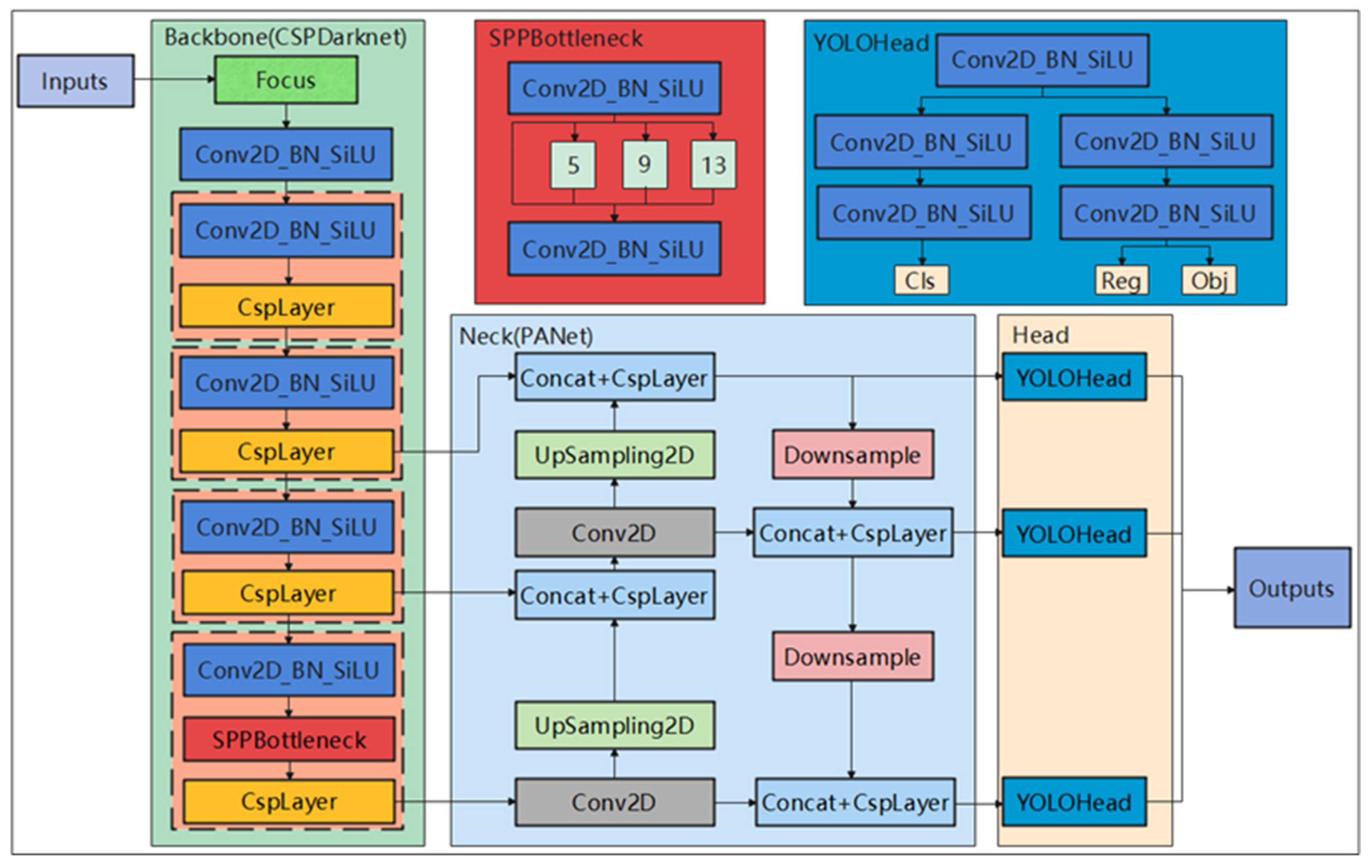
Figure 1. Overall structure of YOLOX algorithm.
Applsci 12 12876 g001
Figure 2. Improved YOLOX network structure.
Applsci 12 12876 g002
Figure 3. Backbone network of Swin Transformer.
Applsci 12 12876 g003
Figure 4. Swin Transformer network structure.
Applsci 12 12876 g004
Figure 5. CBAM network structure.
Applsci 12 12876 g005
Figure 6. Channel attention structure diagram.
Applsci 12 12876 g006
Figure 7. Spatial attention structure diagram.
Applsci 12 12876 g007
Figure 8. (a) Calculation process of SC; (b) Calculation process of DSC.
Applsci 12 12876 g008
Figure 9. GSConv structure diagram.
Applsci 12 12876 g009
Figure 10. (a) Structure of the Gsbottleneck module; (b) Structure of the VoV-GSCSP module.
Applsci 12 12876 g010
Figure 11. Loss values for training.
Applsci 12 12876 g011
Figure 12. PR curves of different models.
Applsci 12 12876 g012aApplsci 12 12876 g012bApplsci 12 12876 g012c
Figure 13. (a) Detection results of different algorithms in a darker environment with more visible flame and less visible smoke; (b) Detection results of different algorithms in a brighter environment with more visible smoke and less visible flame; (c) Detection results of different algorithms in a brighter environment with no flame and more visible smoke; (d) Detection results of different algorithms in a brighter environment with both flame and smoke visible.
Applsci 12 12876 g013
Table 1. Classification results of the dataset at training.
DatasetsTotal Number of Pictures
Training sets4000
Validation Sets500
Test Sets500
Total5000
Table 2. Final training loss function values for different improvement methods.
MethodsSwin-TransformerCBAMSlim NeckLoss Value
YOLOX×××3.66
Improvement1××3.05
Improvement2××3.60
Improvement3××3.49
Improvement4×2.94
Improvement5×2.88
Improvement6×2.91
Improvement72.72
Table 3. Comparison of mAP for ablation experiments.
MethodsSwin-TransformerCBAMSlim NeckmAPtest
YOLOX×××86.17%
Improvement1××90.52%
Improvement2××87.13%
Improvement3××86.30%
Improvement4×91.48%
Improvement5×90.72%
Improvement6×91.48%
Improvement792.26%
Table 4. Comparison of evaluation indexes of different models.
ModelsfireF1smokeF1firePsmokePfireRsmokeRfireAPsmokeAPmAP
SSD74%61%85.05%81.40%65.29%48.99%77.37%64.82%71.09%
Faster R-CNN82%74%86.28%81.32%77.85%67.89%85.40%78.76%82.08%
YOLOv476%67%87.20%80.99%67.80%57.06%78.96%70.90%74.93%
YOLOv581%71%87.13%83.83%76.50%61.83%84.44%76.93%80.68%
YOLOX85%77%87.52%81.80%82.42%73.39%88.65%83.68%86.17%
Improvement YOLOX89%87%90.99%87.78%87.89%86.97%92.78%92.46%92.26%
Publisher’s Note: MDPI stays neutral with regard to jurisdictional claims in published maps and institutional affiliations.