Article

A Denoising Method for Seismic Data Based on SVD and Deep Learning

1
State Key Laboratory of Ore Deposit Geochemistry, Institute of Geochemistry, Chinese Academy of Sciences, Guiyang 550081, China
2
College of Resources and Environment, University of Chinese Academy of Sciences, Beijing 100049, China
*
Author to whom correspondence should be addressed.
Appl. Sci. 2022, 12(24), 12840; https://doi.org/10.3390/app122412840
Submission received: 26 October 2022 / Revised: 1 December 2022 / Accepted: 9 December 2022 / Published: 14 December 2022
(This article belongs to the Topic Research on the Application of Digital Signal Processing)

Abstract

:
When reconstructing seismic data, the traditional singular value decomposition (SVD) denoising method has the challenge of difficult rank selection. Therefore, we propose a seismic data denoising method that combines SVD and deep learning. In this method, seismic data with different signal-to-noise ratios (SNRs) are processed by SVD. Data sets are created from the decomposed right singular vectors and data sets divided into two categories: effective signal and noise. The lightweight MobileNetV2 network was chosen for training because of its quick response speed and great accuracy. We forecasted and categorized the right singular vectors by SVD using the trained MobileNetV2 network. The right singular vector (RSV) corresponding to the noise in the seismic data was removed during reconstruction, but the effective signal was kept. The effective signal was projected to smooth the RSV. Finally, the goal of low SNR denoising of two-dimensional seismic data was accomplished. This approach addresses issues with deep learning in seismic data processing, including the challenge of gathering sample data and the weak generalizability of the training model. Compared with the traditional denoising method, the improved denoising method performs well at removing Gaussian and irregular noise with strong amplitudes.

1. Introduction

Suppressing noise to improve the quality of seismic signals has always been an essential task in seismic data processing. The denoising method for seismic data with a low signal-to-noise ratio (SNR) is a focus of attention at present [1,2]. The traditional methods for denoising seismic data include f-x deconvolution filtering [3,4], t-x prediction filtering [5,6], s-transformation filtering [7], wavelet transform filtering [8], median filtering [9,10], empirical mode decomposition [11], and singular value decomposition. The principle of the singular value decomposition (SVD) method assumes that the effective seismic information is mainly concentrated in the feature maps corresponding to large singular values. The effect of noise attenuation can be achieved by setting K = 1 or K = 2 when reconstructing. The traditional seismic data denoising methods are very effective when the SNR is high, but they are unsuitable for low SNR seismic signals. For example, SVD is used to remove seismic data noise. When the noise energy is too large, the large singular value may not represent the effective signal. At this time, it is difficult to choose the rank. When the rank is too large, too much noise will be retained, and the seismic signal becomes damaged when the rank is too small. So choosing the appropriate rank is a crucial step for the SVD method [12,13]. Therefore, exploring a method that can effectively attenuate the noise of seismic data with a low SNR is necessary.
Currently, the research on the denoising of seismic data using the SVD method is continuing, and there are some advances in the suppression of strong amplitude, random, coherent, and abnormal optical noise. For example, Ke Chen et al. [14] proposed a singular spectrum analysis method using low-rank approximation instead of truncated SVD to suppress intense interference noise. To compress and denoise seismic data, Milan Brankovic et al. [15] proposed a shift matrix decomposition (SMD) method that compresses seismic data by applying SVD and storing the seismic data into singular vector pairs coupled with shift vectors. These methods can suppress the noise but only partially remove it in areas without a seismic signal. However, the improved SVD method proposed by us can remove the noise in an area without a seismic signal. Qian Kun Feng et al. [16] proposed a multi-channel SVD denoising convolution neural network, which remarkably removes random, correlated, and optical abnormal noise. However, compared with the right singular vector, noise subspaces’ records are morphologically complex, which makes it more difficult to make data sets and identify seismic signals. Meanwhile, the training time of the network is longer, and the computer performance requirements are high. However, in our proposed method, the right singular vector is simple in form, easy to collect, fast in training time, and low in computer performance. Chao Qiang Xi et al. [17] used a Wiener filter based on SVD to attenuate coherent noise. In this paper, the SVD technique is improved for Gaussian noise and irregular intense amplitude noise in seismic data so that the new method effectively suppresses the noise.
Considering the vast and successful application of deep learning methods in various fields, many applications in seismic exploration include seismic data denoising, seismic fault detection, seismic signal reconstruction, and seismic signal classification. For example, Yu Shu Zhang et al. [18] improved the deep convolution neural network based on a patch and used it to denoise seismic images. This method dramatically affects seismic data with a low SNR and noise that changes randomly with time and space. Xin Ming Wu et al. [19] used a supervised full convolution neural network for 3D seismic image recognition, thus enabling accuracy and efficiency in predicting the location of faults. Jin Sheng Jiang et al. [20] developed a convolutional self-coding method that can remove random noise while reconstructing seismic signals and quickly process a large amount of seismic data. Bing Jun Li et al. [11] classified effective signals using ensemble empirical mode decomposition and deep convolution neural networks. Firstly, the empirical ensemble mode decomposed the seismic signals, and the modal function components obtained the three-dimensional Hilbert spectrum using the Hilbert transform. Then, the three-dimensional Hilbert spectrum was used as a training set for the deep convolutional neural network. The Hilbert spectra of natural earthquake and explosion signals were predicted after training, obtaining excellent results. Yun Zhi Shi et al. [21] classified seismic images into saline and non-saline datasets on a patch-by-patch method. They used the trained deep convolution neural network to automatically capture subtle salt features from 3D seismic images. Xinxin Yin et al. [22] proposed a lightweight unsupervised network that combines a convolutional neural network and an unsupervised classification method. The method improves computational efficiency and achieves excellent classification results by extracting signal features to classify seismic signals.
Seismic data denoising methods based on deep learning have achieved significant advancements and found widespread use compared with traditional seismic data denoising methods. However, it is difficult to gather sample seismic data because the deep learning denoising method requires a large amount of labeled seismic data to train the network. The trained model has weak generalization ability, which significantly limits the use of deep learning networks in denoising seismic data [19].
In this paper, two-dimensional seismic data were denoised using SVD combined with supervised deep learning techniques. The singular vectors after SVD also exhibited characteristics that discriminate between noise and effective signals, as demonstrated by Wang Chao et al. [12]. We used their study as a foundation, to develop a supervised deep learning technique that automatically determines the right singular vector (RSV) relating to noise and effective signal. Only the RSV corresponding to effective signals were used to reconstruct the seismic data.

2. Method

2.1. Singular Value Decomposition (SVD)

The SVD can perform principal component decomposition and is widely used in seismic data noise reduction. The complete singular value decomposition formula is:
D m × n = USV T = K = 1 R u k σ k v k T
The D matrix has m sampling points for each channel and n channels. R denotes the rank of the matrix D, U the orthogonal matrix of m × m , V the orthogonal matrix of n × n , S the diagonal matrix of m × n ; σ k is singular value and is arranged in order from highest to lowest in the S-matrix. The left singular vector (LSV) is designated by u k and, the RSV by v k . See Appendix A for details.
D m × n = USV T = K = 1 R u k σ k v k T = u 1 σ 1 v 1 T + u 2 σ 2 v 2 T + + u R σ R v R T
The matrix D decomposes into R submatrices. Since the seismic signal is continuous in space, the noise is randomly distributed. The higher singular value often reflects the effective signal. The lower singular value generally represents the noise. As a result, the singular value can be used to distinguish between the noise and the effective signal.
D m × n = USV T = K = 1 r u k σ k v k T   1 r R
K is frequently adjusted to 1 or 2 when reconstructing seismic data. The reconstruction error of seismic data is the sum of the matrix corresponding to the remaining singular values. By using SVD, it is discovered that the LSV and RSV of 2D seismic data indicate various physical meanings. The RSV indicates the lateral variation trend of the amplitude of the seismic lineups, whereas the LSV represents the seismic wavelet. The first left singular vector typically represents the normalized wavelet of the seismic signal to the seismic data after SVD. At the same time, the noise is represented by the following columns of LSV. Similarly, the first right singular vector indicates the amplitude variation of the effective signal, whereas the variations of the remaining RSV are more random and represent noise [12,16].
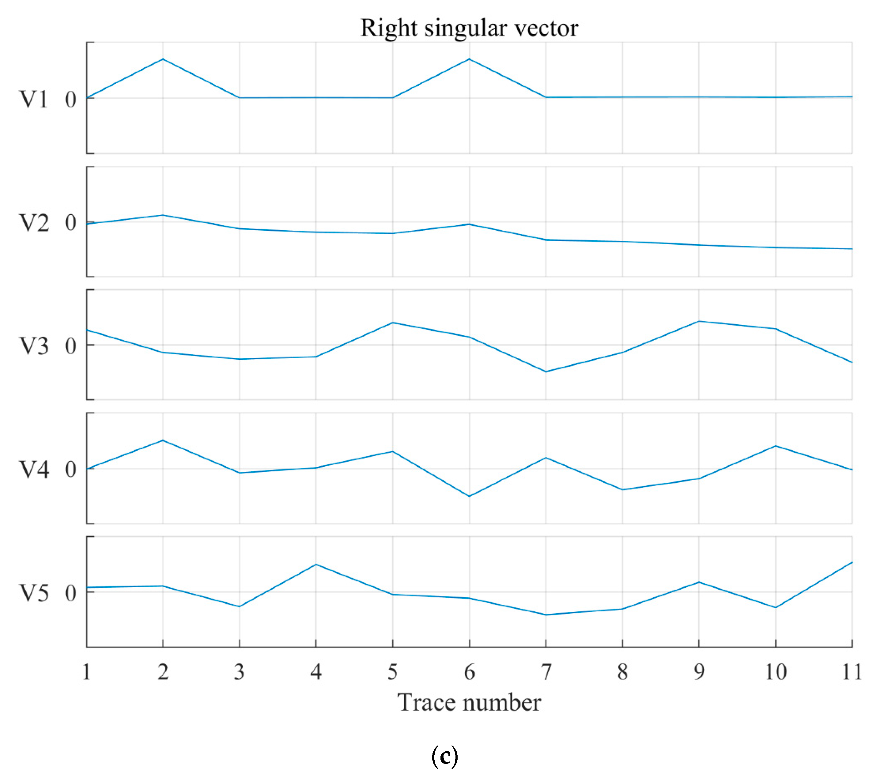
However, the seismic signal becomes significantly disturbed by intense noise. Figure 1a shows intense amplitude noise in the 2nd and 6th seismic data. The seismic data are decomposed by SVD, as shown in Figure 1b. The first LSV represents noise, and the second represents the effective signal. The traditional singular value method cannot denoise seismic data in this case. In Figure 1c, the first RSV correspondingly represents the amplitude change of seismic data, in which sizeable abrupt change represents intense amplitude noise. By contrast, the absolute value of the second RSV generally shows an increasing trend, which confirms that seismic signal amplitude gradually increases.
The RSV characteristics corresponding to noise and effective signal are very different. Therefore, we could distinguish the effective signal and noise based on the RSV characteristics in addition to the singular value. As a result, flexible control over the rank selection of seismic data reconstruction was possible. The goal of intelligent noise suppression was finally accomplished.

2.2. Denoising Method Based on SVD and Deep Learning

Since the decomposed LSV and RSV have clear physical significance related to seismic data, the effective seismic signal and noise can be well distinguished using the decomposed RSV characteristics [12]. It is easy to manually distinguish a seismic signal or noise according to the RSV characteristics. However, the conventional mathematical or signal processing methods proposed by Wang Chao et al. [12] cannot reach the high-accuracy judgment requirement. By contrast, deep learning has significant advantages in dealing with such problems. Deep learning has developed mature classification abilities. Therefore, this paper uses the MobileNetV2 classification network [23] to predict and classify the right singular vector after SVD. The basic idea is that two-dimensional seismic data with different SNR sizes are subjected to SVD, and the obtained RSVs are transformed into graphs. The images are classified to make a dataset training network model. The trained deep learning model distinguishes the effective signal and noise corresponding to the RSV of seismic data after SVD. Then, the singular value corresponding to the noise is rejected, and the effective signal is retained and smoothed. Finally, denoised two-dimensional seismic data are obtained by SVD reconstruction, and the purpose of denoising is finally achieved (Figure 2).

2.2.1. Selection of Deep Learning Networks

Deep learning has become increasingly sophisticated in image classification, and convolutional neural networks (CNNs) are widely used in image classification with good results. Many convolutional neural networks exist, including Alex Net [24], VGG Net [25], Res Net [26], Dense Net [27], and MobileNet [28]. Each type of neural network has unique advantages and is suitable for different environments. A suitable neural network can be selected according to the application environment and the neural network’s characteristics.
There are many types of deep learning networks, and two of the better-known classification networks, MobileNetV2 and restnet50 were selected for comparison here. The network was run on an NVIDIA GeForce GTX 750 Ti computer with a GPU of 2 GB. The restnet50 network had a maximum batch size of 8. The MobileNetV2 network had a maximum batch size of 16. The rest of the training parameters were the same as those used to train the MobileNetV2 network below (see Section 2.2.3).
Our results are shown in Table 1. The restnet50 network requires twice the time to train and has slightly lower accuracy than the MobilenetV2 network. Compared to standard convolutional operations, the MobileNetV2 network can reduce the amount of computation by a factor of several with the same weight parameters, thus achieving a speed-up of network operations. Therefore, the MobilenetV2 network was finally selected for its fast training speed, high accuracy, few training parameters, and low-performance requirements.

2.2.2. Deeply Separable Convolution in MobileNetV2 Networks

Deeply separable convolution is a crucial part of the MobileNet network and its ability to operate efficiently. Deeply separable convolution is divided into two parts, the depthwise and pointwise convolutions. Depthwise convolution is the process of extracting features from an image using a single convolution channel to produce an output feature map that maintains the same channel as the input feature map. Pointwise convolution refers to the up-and down-dimensioning of the feature map by 1 × 1 convolution. The network can achieve the same results as standard convolution with fewer parameters and operations by replacing standard convolution with these two components [23].
The number of parameters and operations in the deeply separable convolution is 1 N +   1 H i 2 times the number of parameters of the standard convolution, where the number of convolution kernels is N, and the size of the convolution kernel is H i . The H i in the MobileNetV2 network is 3, so the network has eight to nine times less computation than the standard convolution, reducing the number of operations to a large extent [23].
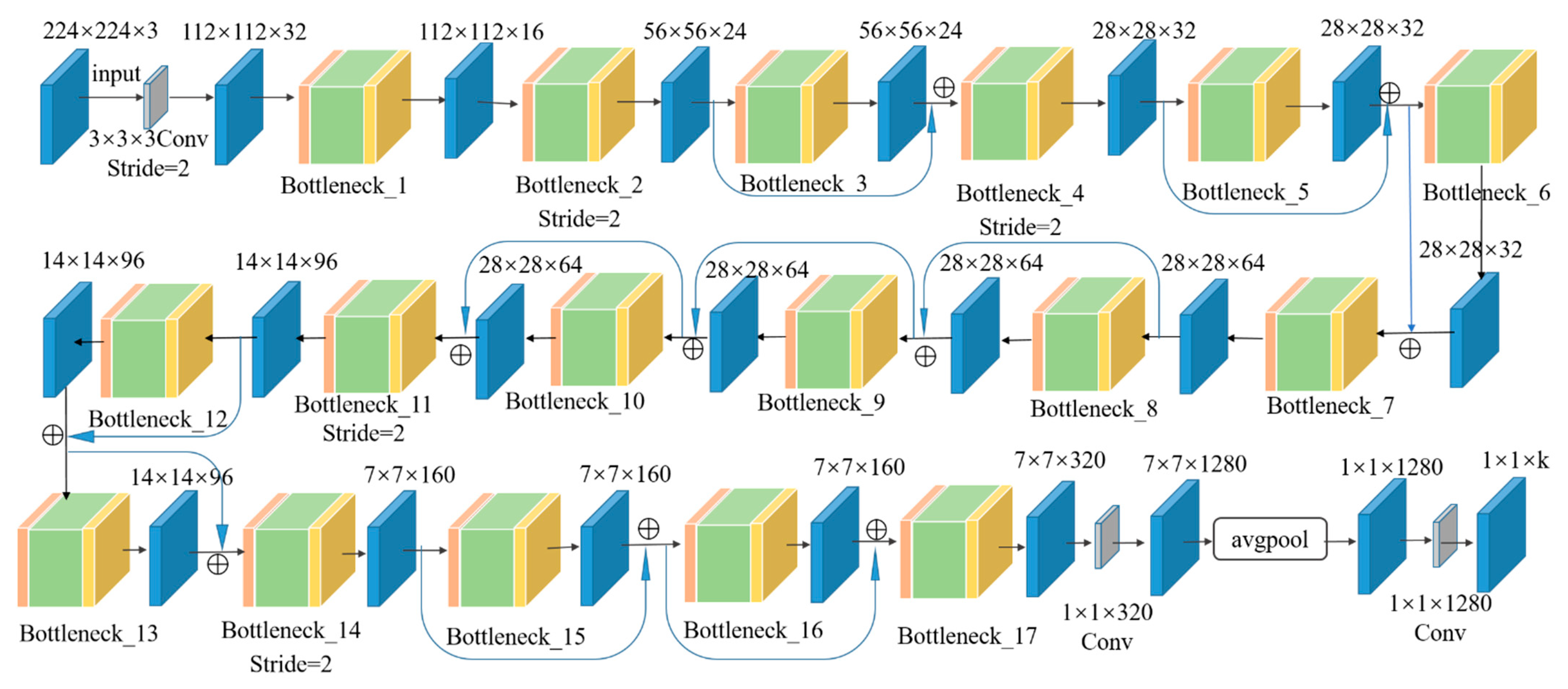
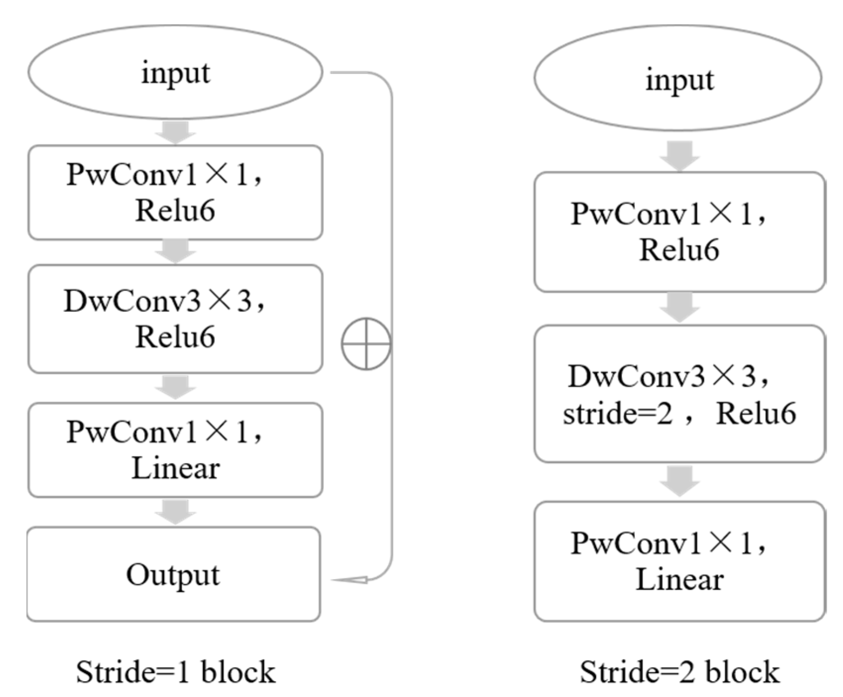
The MobileNetV2 network structure is shown in Table 2 and Figure 3, with 17 bottleneck layers, 1 standard convolutional layer (Conv), and 2 pointwise convolution layers (Pw Conv), for a total of 54 trainable parameter layers. Figure 4 shows a bottleneck layer containing two pointwise convolutional layers and one depthwise convolutional layer (Dw Conv). When the bottleneck layer step size is 1, the training images are first up-dimensioned by 1 × 1 convolution, and then depthwise convolution is performed to extract features. Finally, the input and output are summed up by linear pointwise convolution, forming the residual structure. When the bottleneck layer step size is 2, the shortcut structure is not added because the input size does not match the output, and the rest is consistency. The linear bottleneck and inverted residuals used in the MobileNetV2 structure optimize the network, resulting in deeper layers, smaller models, and faster runs [23].

2.2.3. MobileNetV2 Network Training

The data for the production dataset comprised three synthetic seismic data with 267 channels of 2048 sampling points per channel and 31 channels of 4200 sampling points per channel of field seismic data. SVD processed the seismic data, and then the right singular vector was transformed into a graph with a picture size of 224 × 224 pixels. Finally, the generated images were divided into two categories, effective signal and noise. It was built into a dataset of 10,468 training photos and 3416 validation images, representing approximately 75 and 25% of the training and validation sets, respectively.
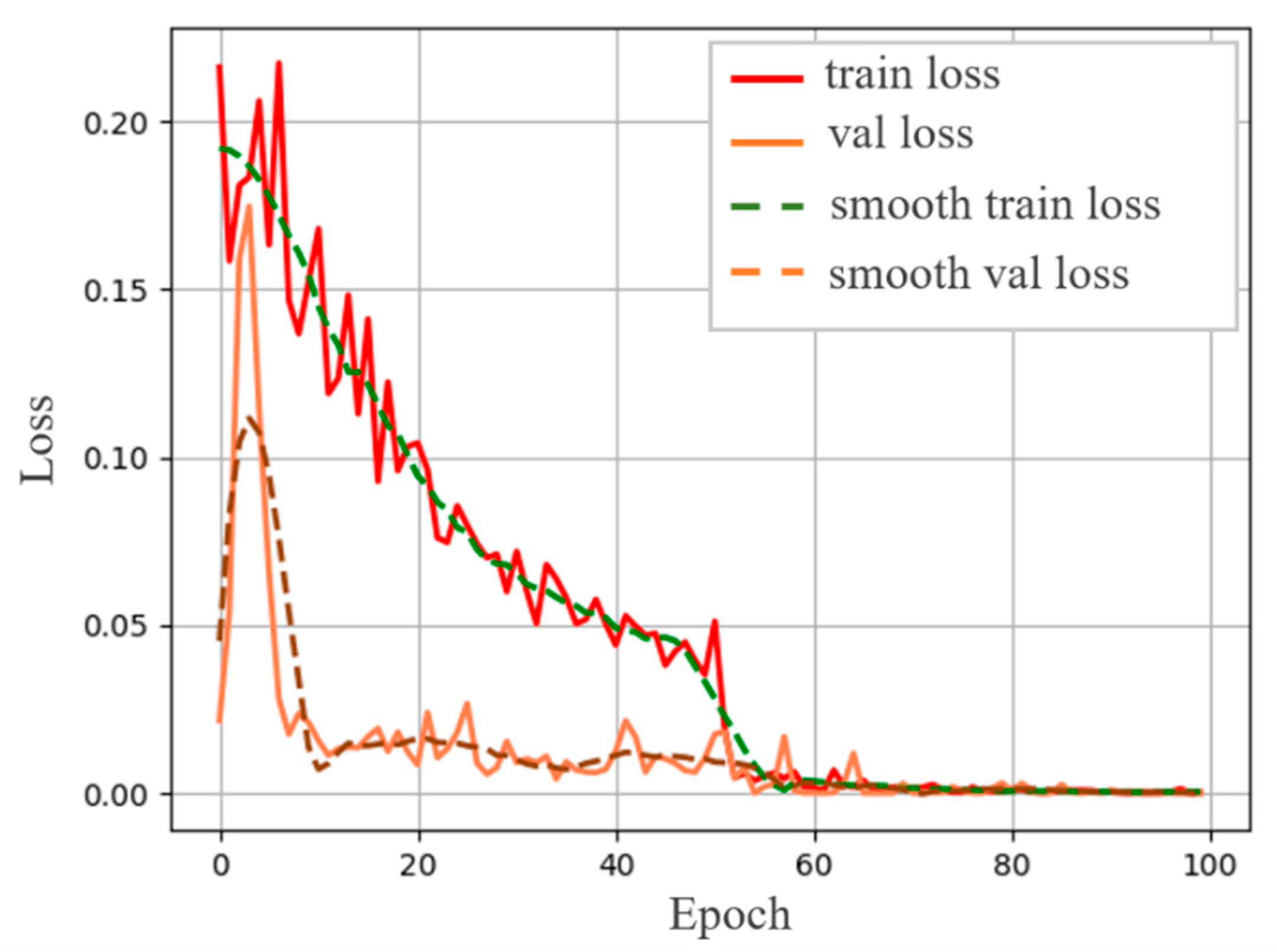
The network model was trained on the computer using the PyTorch deep learning framework and by setting the batch size to 16. The training network was divided into two phases: the freezing phase and the thawing phase, and the backbone part extracted the generic network features. Freeze training can speed up the training speed and prevent the weights from being destroyed early in training. We set the learning rate to 0.01, and the epoch to 50 in the freeze phase. The learning rate and epoch of the thawing phase were set to 0.0001 and 50, respectively. The accuracy of the training set did not significantly increase after epoch 70 over the 100-epoch training process, and the final accuracy of the validation set was 99.94%.
The rate of convergence of the MobileNetV2 network for image categorization is shown in Figure 5. The training set had large initial fluctuations and gradually decreased after 20 epochs. The loss of the training set curve after smoothing decreased and gradually smoothened out close to 0 at 70 epochs. According to the validation set’s loss curve, the training of the validation set was initially unstable, and the loss value increased for a while. The loss value gradually and steadily decreased after running for about 5 epochs. Finally, at 70 epochs, the loss value approached 0 gradually and smoothly.
After training the MobileNetV2 network, the network model was used to predict the input images. The input images’ prediction results are shown in Figure 6a–c, which are effective signals represented by the right singular vector. The test results are consistent with the manual prediction results. Figure 6d–f are the noise represented by the right singular vector, which presents a cluttered and random fold. The test results are consistent with the manual prediction results, and the network can accurately determine the effective signal and noise.

2.2.4. Algorithm Program Steps

The process of improving the SVD seismic denoising method is shown in detail in Algorithm 1. This pseudo-algorithm is performed in python.
Algorithm 1 Pseudocode of Seismic Denoising Algorithm
Input: D m , n : seismic data have m traces, n samples, window parameters were set to a traces, b samples, (a is an odd number and b is an even number), rank of matrix K = 4;
Output:  W m , n : denoised seismic data;
  1: W m , n = D m , n ;
  2: for ( a / 2 ) + 1 < i m − a/2 + 1, i + a do
  3:      for (b-1)/2 + 1 < j n − (b − 1)/2, j + 1 do
  4:        Set window = a * b (a < m, b < n), obtain d a , b = D i a 2 : i + a 2 1 , j b 1 2 : j + b 1 2 ;
  5:        Compute SVD function USV = svd(d), obtain U a , a : left singular matrix, S a , b : singular value matrix, V b , b : right singular matrix;
  6:        for 0 < k K do
  7:          Transform the kth RSV into 224*224 pictures;
  8:          Using a trained MobileNetV2 network to predict the kth RSV;
  9:          if V[:,k] = “effective” then
  10:             S[k,k] = S[k,k];
  11:             A five-point smoothing is applied to the kth RSV;
  12:          else V[:,k] = noise”
  13:            S[k,k] = 0;
  14:          end if
  15:       end for
  16:       w a , b = k = 1 K U k S k V K T ;
  17:       Extract the reconstruction matrix w[ : , b 1 2 + 1 ] and insert it into the M[ i a 2 : i + a 2 1 , j ] matrix data;
   18:    end for
   19: end for
   20: Return W m , n .

3. Results

3.1. Synthetic Data

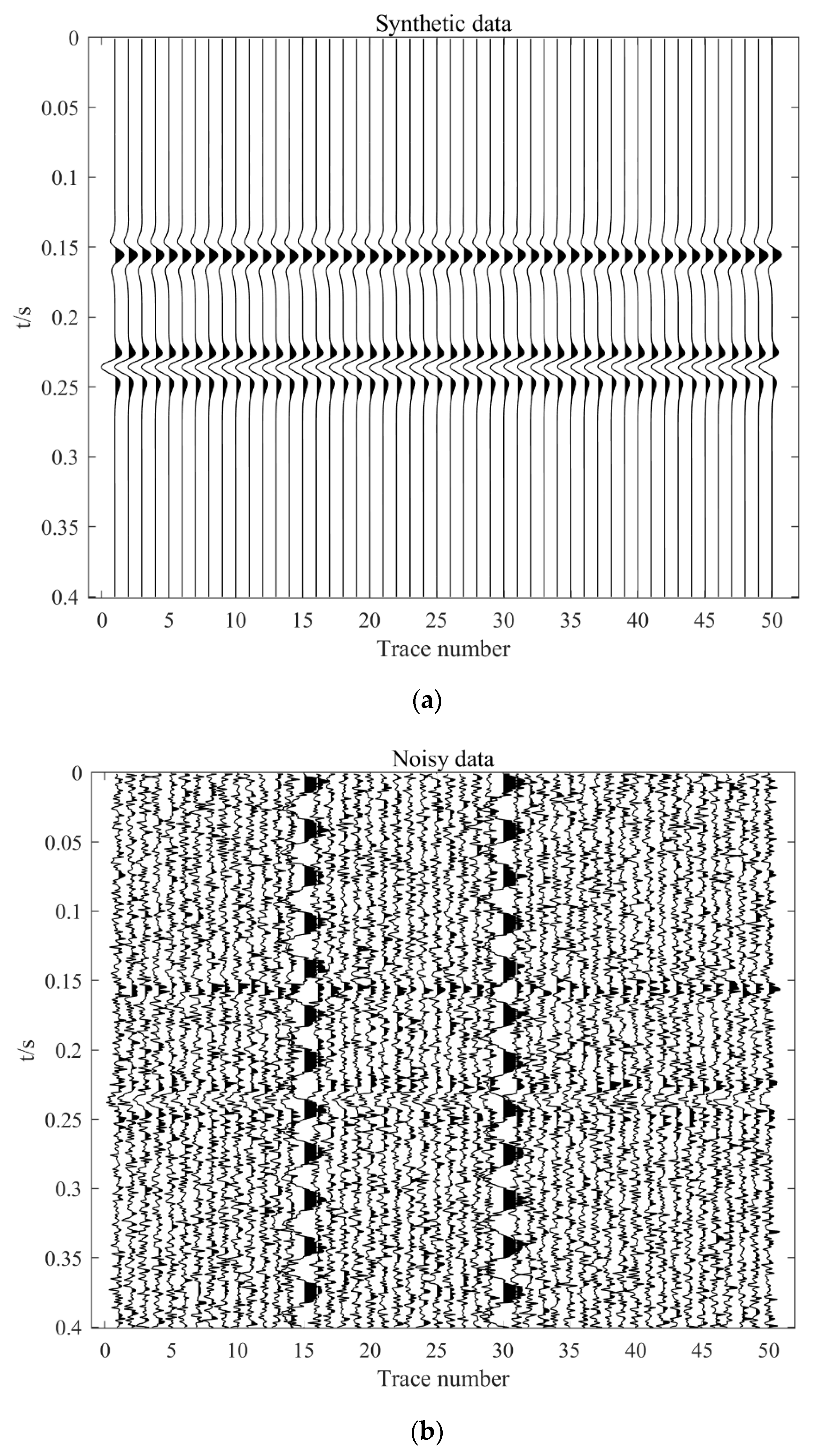
The synthetic 2D seismic data containing 50 traces and 400 sampling points are presented in Figure 7a. Gaussian noise with SNR = −4 was added to the synthetic seismic data, and intense amplitude noise was added to the seismic data of the 15th and 30th channels. The noise negatively impacted the seismic signal, where part of the seismic signal was completely drowned in the noise (see Figure 7b). To denoise the synthetic seismic signal, the seismic data were first reconstructed using the conventional SVD filtering (K = 1 and K = 2). When singular value decomposition filtering was performed to denoise seismic data, K = 1 and K = 2 were the most common because the seismic signal was mainly concentrated on the maximum singular value. Conventional singular value decomposition filtering uses window parameters of n = 15 channels and m = 100 sampling points.
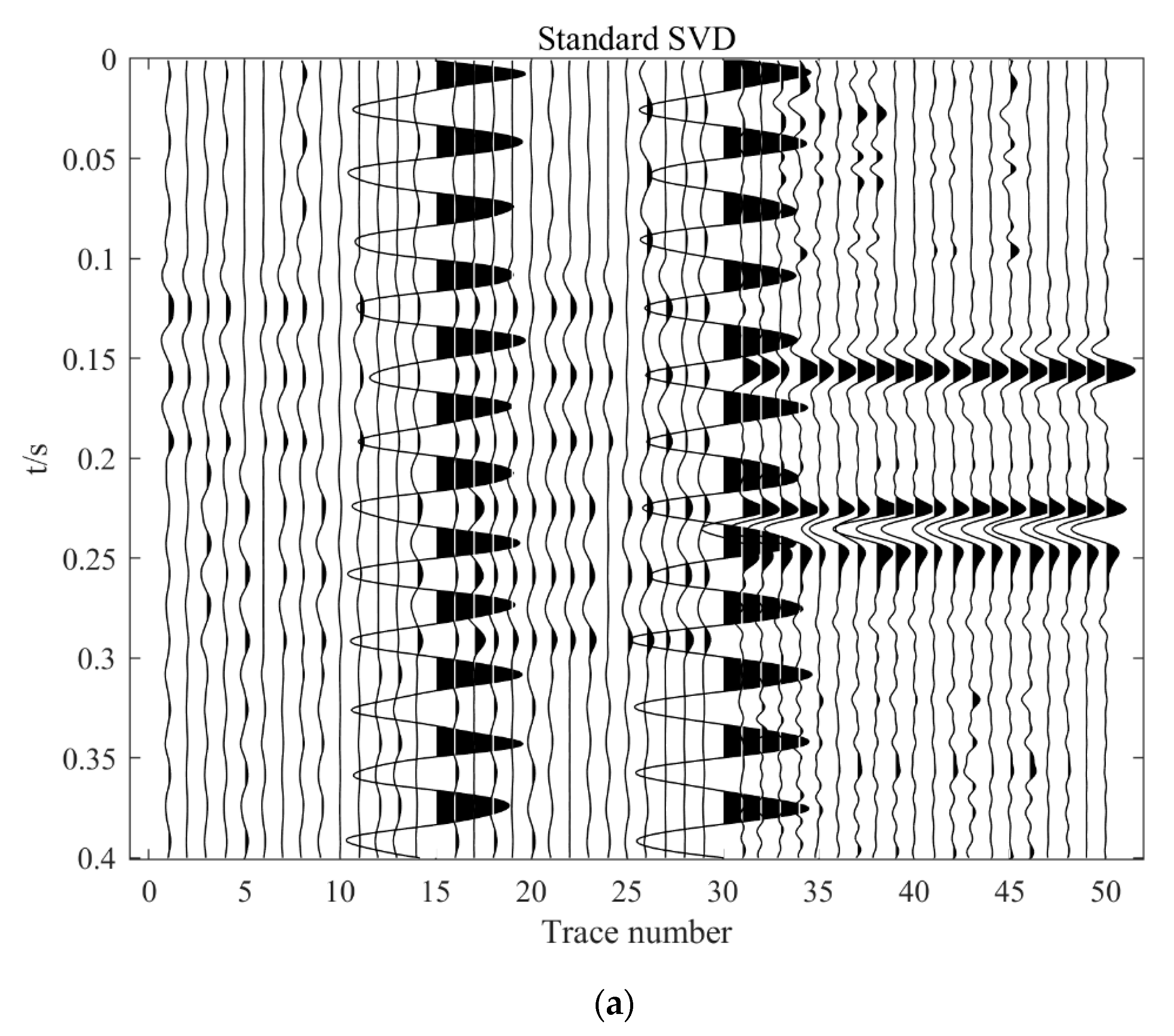
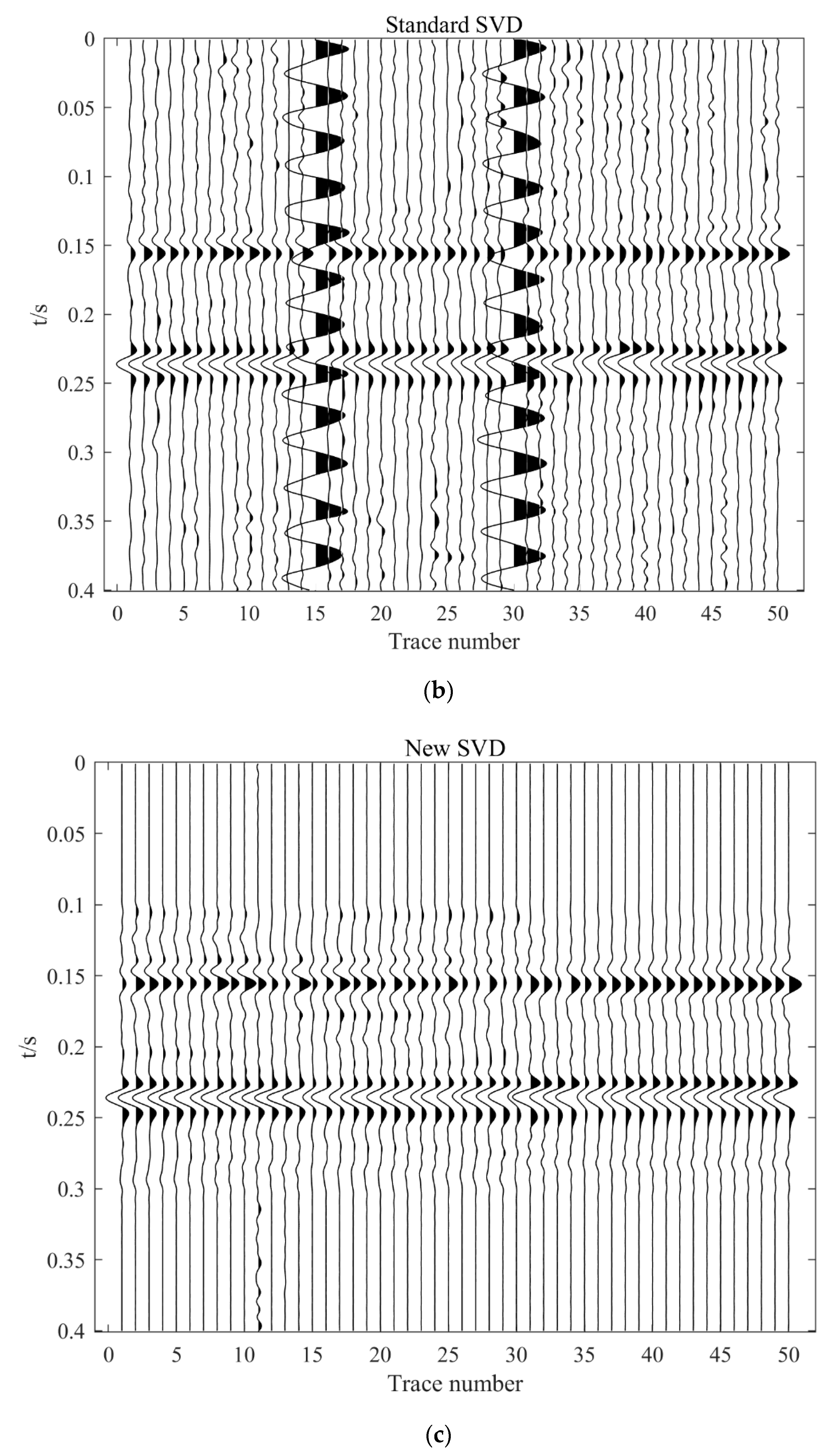
Only the first singular value (K = 1) was used to reconstruct the seismic data. The results are shown in Figure 8a, where the random noise is removed to a large extent. However, the seismic signal is lost on a large scale due to the interference of intense amplitude noise, which is not removed. The conventional SVD filtering results are shown in Figure 8b; the seismic signals are all preserved when K = 2, but it cannot effectively remove the intense amplitude noise. Since the SVD filter does not have low-pass filtering capabilities, the effective frequency band of the synthetic seismic data was between 0 and 100 Hz, and the synthetic seismic data were processed using low-pass filtering (0–100 Hz). The results in the later sections were also after adding low-pass filtering.
When processing seismic data with the modified SVD filter, the window chosen was the same as the conventional SVD filter. The rank range was expanded to select K = 4 for processing. After the improved SVD processed the seismic data, the seismic signals were kept intact, and the intense amplitude noise was removed successfully. In the region without a seismic signal, Gaussian noise was suppressed completely. This result was also discernible in the region with a seismic signal. The continuity of the lineups’ seismic signal was maintained (see Figure 8c).
The comparison of the SNR of different methods is shown in Table 3. The seismic data’s SNR was −10.2592 dB before processing the synthetic seismic data with filling noise. After noise attenuation, the SNR for K = 1 and K = 2 in a conventional SVD filter was −6.8822 dB and −6.5176 dB, respectively. However, the SNR was 8.1007 dB after the seismic data was processed using improved SVD filtering. As a result, we discovered that the improved SVD filter’s ability to suppress noise had improved.

3.2. Field Data

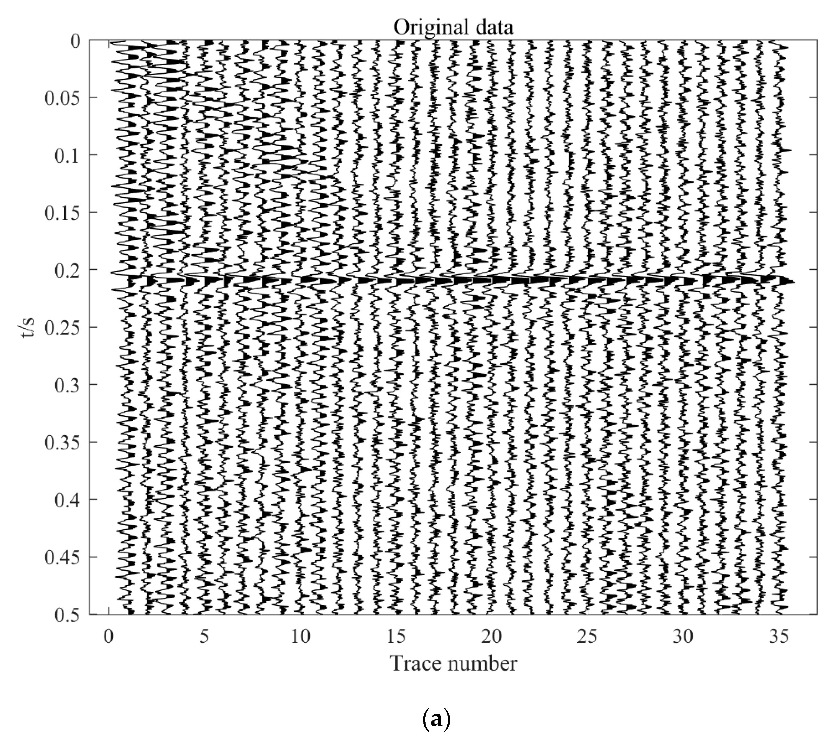
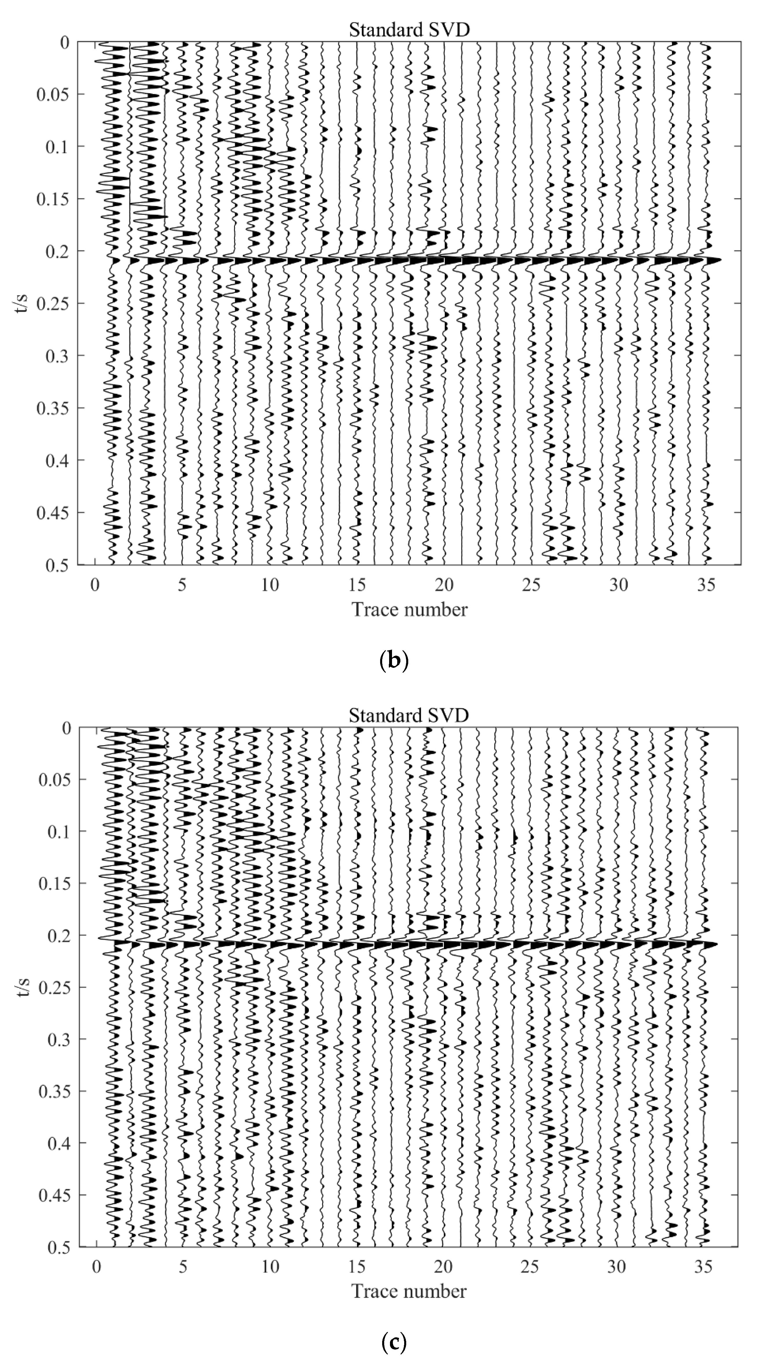
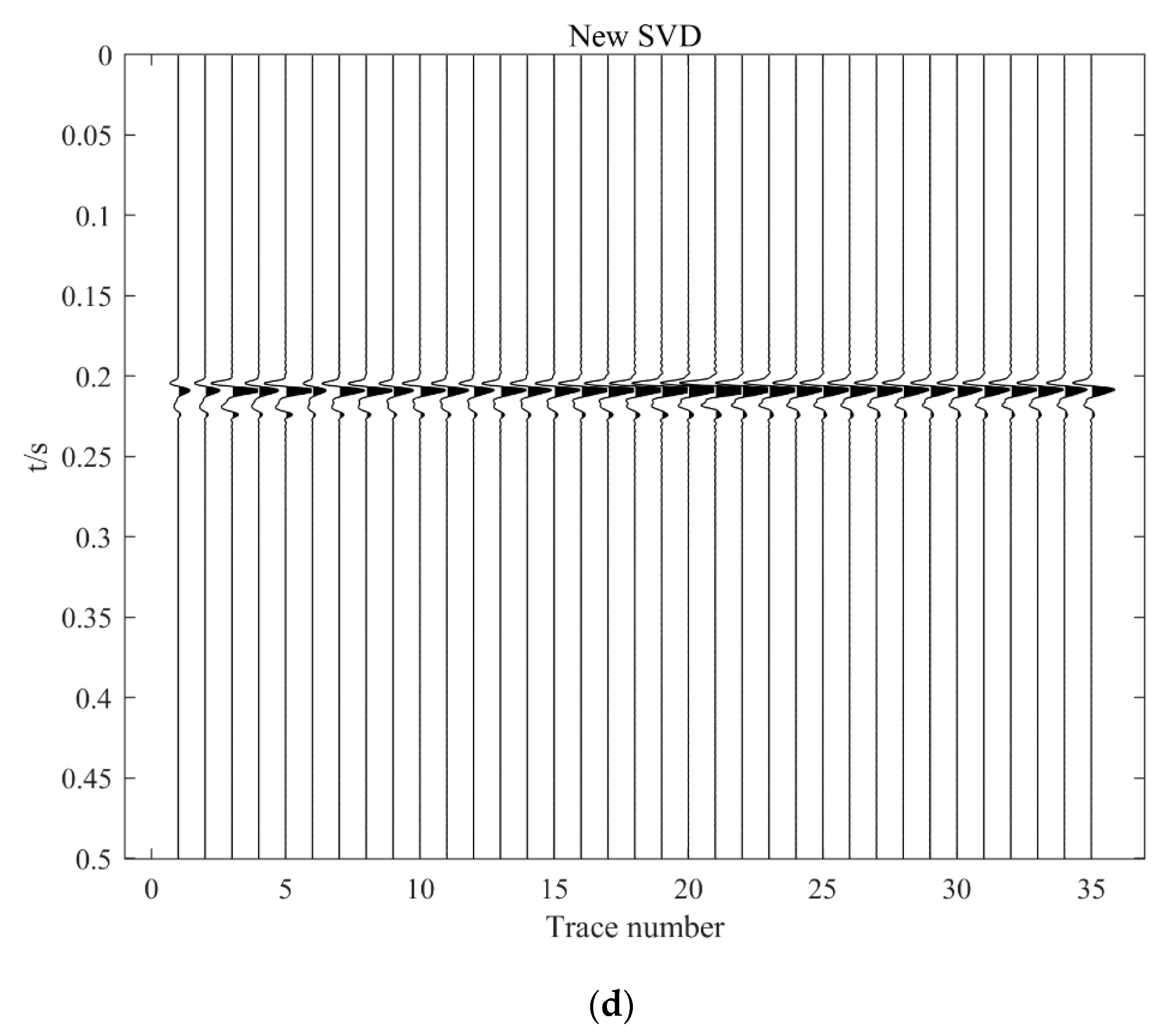
The first field seismic data were obtained by microseismic monitoring in a well with 35 magnitude geophone. The distance between the two geophones is 15 m, and the geophone depth was 1800–2310 m. The sampling rate was 0.5 ms. The downhole microseismic data has 35 traces and time length is 0.5 s. The field seismic data has robust random noise and apparent intense amplitude noise, as shown in Figure 9a. When denoising the field data, the parameters of the used window were set to n = 15 traces and m = 50 time samples, and the other parameters chosen for the improved SVD filtering were the same as those used for processing synthetic seismic data. As seen in Figure 9b, a large amount of random noise is removed when traditional SVD filtering (k = 1) is used. However, a significant amount of noise still exists near the non-effective signal. When performing SVD filtering denoising with K = 2, the retained noise is more relative to K = 1, as illustrated in Figure 9c. The conventional SVD filtering (K = 1 and K = 2) minimally suppresses intense amplitude noise. However, the noise was eliminated in the region without seismic signals when the data were denoised by the improved SVD filtering. When the noise was attenuated, the seismic events were well preserved in the vicinity of the seismic signal, and the intense amplitude noise was eliminated (see Figure 9d). In general, the improved SVD filtering significantly improves the denoising of seismic data compared with conventional SVD filtering. Here, the results of SVD filtering were processed using low-pass filtering from 0 to 240 Hz.
Since SNR cannot be calculated directly from field seismic data, the SNR of field seismic data and denoised seismic data were calculated by taking 0.2–0.225 s as seismic signal and 0.35–0.375 s as noise. The SNR of field seismic data is 11.3336 dB. After denoising the seismic data with the traditional SVD filter (K = 1, K = 2), the SNR of the seismic data is 18.5297 dB and 16.8173 dB, respectively. After the improved SVD filter was used to denoise the seismic data, the noise part was basically removed, so there was a numerical calculation error, and the SNR of the seismic data was 65.7588 dB. The comparison of SNR shows that the improved SVD filter has an obvious denoising effect (Table 4).
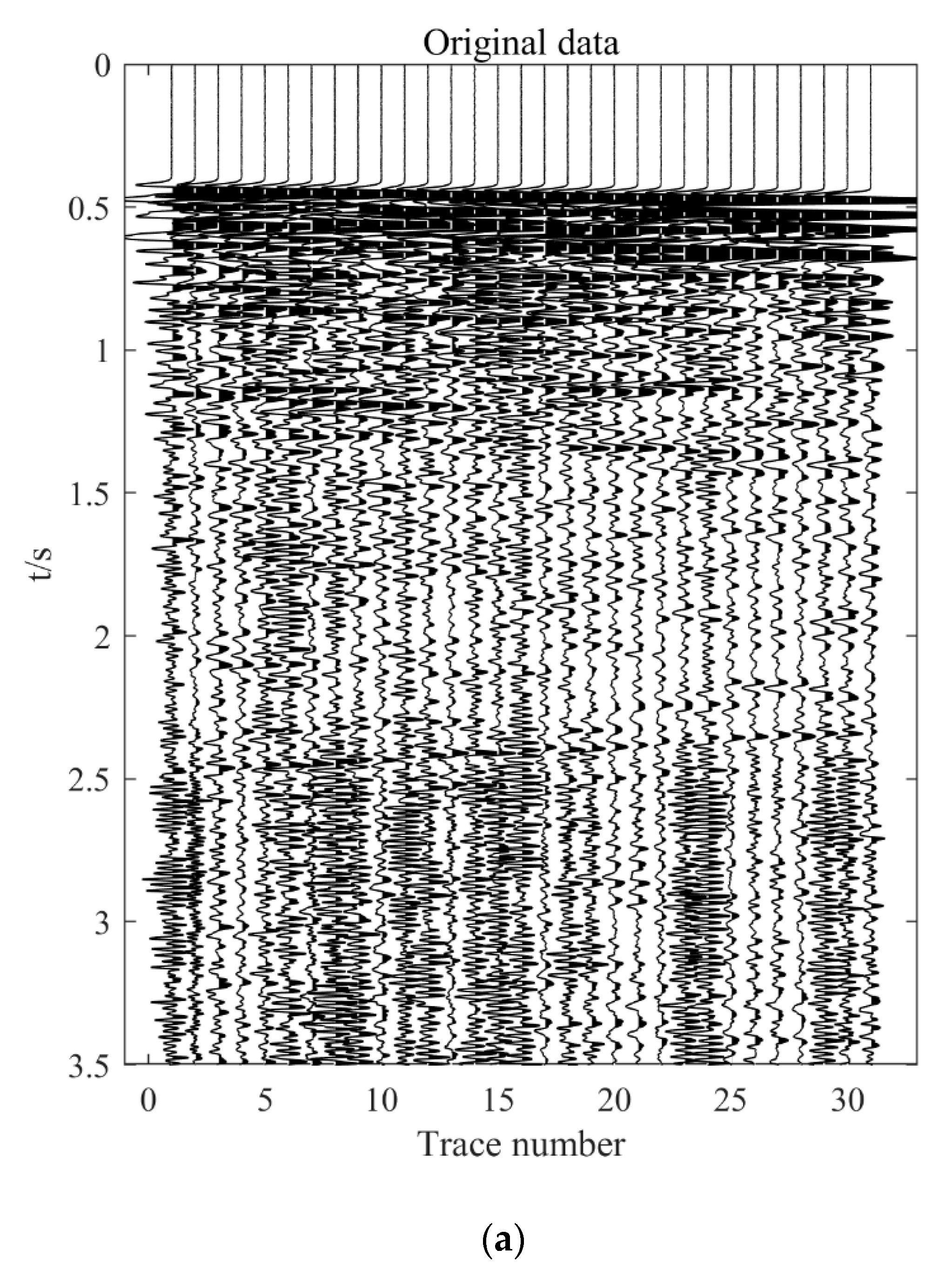
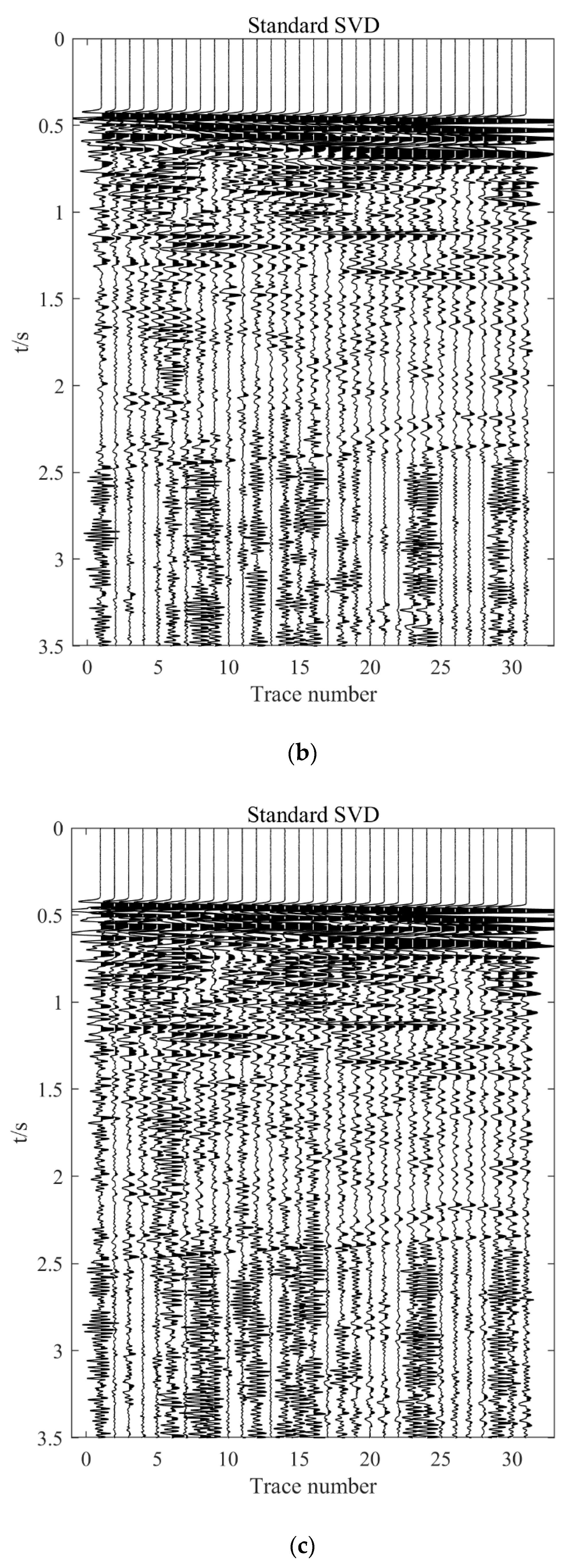
The second field seismic data were obtained by 31 magnitude geophones with a level spacing of 15 m and the depth of the geophone sinking was 1800–2250 m; the explosive source was placed in the adjacent well. The sampling rate was 1 ms. This downhole microseismic data comprised 31 traces and time length was 3.5 s. In Figure 10a, it can be seen that the 0.5 to 2 s contains a large amount of random noise, and there is erratic intense amplitude noise from 2.5 to 3.5 s. The parameters chosen for the improved SVD filtering were the same as those used to process the synthetic seismic data. The filtered results were compared to the conventional SVD filtering results. Figure 10b shows the denoised data obtained using conventional SVD filtering (K = 1). Most random noises were suppressed, but the erratic intense amplitude noise from 2.5 to 3.5 s could not be attenuated. At the same time, the seismic events near 2.5 s were also discontinuous and partially missing due to the interference of intense amplitude noise. After denoising the data with conventional SVD filtering (K = 2), the seismic signal was preserved, but the noise was also present. The conventional method did not achieve the effect of noise suppression (see Figure 10c). The noise was mainly removed from the seismic data by the improved SVD filtering rather than the original method. The irregular intense amplitude noise from 2.5 to 3.5 s was attenuated. The seismic events with complex characteristics were better preserved (Figure 10d).

4. Discussion

In this paper, we propose a two-dimensional seismic data denoising method combining SVD and deep learning. This method attenuates strong interference noise, which cannot be completely removed with traditional SVD filters, and resolves discontinuous weak seismic signals when the effective signal and noise are distinguished only according to the singular value. The improved SVD filtering technology can improve the low efficiency of artificial rank selection and the accuracy and effectiveness of noise suppression.
When SVD is applied to 2D seismic data, only the effective signal and noise are distinguished based on the RSV. The effective signal and noise patterns corresponding to the RSV are rather straightforward compared with field seismic data, reducing the challenge of obtaining sample data. The morphological complexity and number of RSV categories after SVD are significantly reduced compared with the complex and varied seismic data. The morphological characteristics of the RSV corresponding to different seismic data do not vary significantly. Improved SVD filtering effectively overcomes the weak generalization ability of the deep learning training model. Compared with traditional SVD filtering, the improved SVD filtering successfully eliminates Gaussian noise and strong amplitude noise in the synthetic seismic data. It maintains the integrity of seismic events in the field of seismic data. However, the disadvantage is that the seismic data targeted are single, mainly for horizontal lineups. Our future work will denoise seismic data containing cross and inclined lineups.

Author Contributions

Conceptualization, G.J. and C.W.; methodology, C.W.; software, G.J.; validation, G.J.; formal analysis, G.J.; resources, C.W.; data curation, G.J.; writing—original draft preparation, G.J.; writing—review and editing, C.W.; visualization, G.J.; project administration, C.W.; funding acquisition, C.W. All authors have read and agreed to the published version of the manuscript.

Funding

This research was funded by the National Natural Science Foundation of China, (41874166), and the Guizhou Science and Technology Cooperation Platform Talents Program ([2021]5629).

Institutional Review Board Statement

Not applicable.

Informed Consent Statement

Not applicable.

Data Availability Statement

The data of this study is available from the authors upon request.

Acknowledgments

We thank the support provided by the Guizhou Science and Technology Cooperation Platform Talents Program of China ([2021]5629) and the National Natural Science Foundation of China (41874166). At the same time, we also thank the reviewers for their valuable time. The results of this study and codes are available from the authors upon request.

Conflicts of Interest

The authors declare no conflict of interest.

Appendix A

The formula for SVD is as follows:
D = US V T
D is a matrix of m × n, and U is a matrix of m × m. S is a matrix of m × n, S is 0 except for the elements on the main diagonal, and each element on the main diagonal is called a singular value σ k . V is a matrix of n × n and U T U = I, V T V = I.
( D T D ) v k   =   λ k v k
From the above formula, we can get n eigenvalues and n eigenvectors of D T D . All eigenvectors of D T D form matrix V and each eigenvector of V is called the right singular vector.
( DD T ) μ k   =   λ k u k
From the above formula, m eigenvalues and m eigenvectors of DD T can be obtained. All eigenvectors of DD T form a matrix U, and each eigenvector of U is called the left singular vector.
D T = VS U T D T D = VS U T USV T = V S 2 V T σ k = λ k
Hereߣs an example of the definition matrix D is:
D = 1 2 2 1 1 1
D T D = 1 2 1 2 1 1 1 2 2 1 1 1 = 6 5 5 6
DD T = 1 2 2 1 1 1 1 2 1 2 1 1 = 5 4 3 4 5 3 3 3 2
The eigenvalues and eigenvectors of D T D can be found:
λ 1 = 11 ;   v 1 = 1 2 1 2 ;   λ 2 = 1 ;   v 1 = 1 2 1 2 ;
The eigenvalues and eigenvectors of DD T can be found:
λ 1 = 11 u 1 = 3 2 3 2 1 ;   λ 2 = 1 ,   u 2 = 1 1 0 ;   λ 3 = 0 ,   u 3 = 1 3 1 3 1 ;
From σ k = λ k , we know that the singular values are 11 and 1, so we get a singular value decomposition of D:
D   =   US V T   =   3 2 1 1 3 3 2 1 1 3 1 0 1 11 0 0 1 0 0 1 2 1 2 1 2 1 2

References

  1. Lin, H.; Wang, S.; Li, Y. A Branch Construction-Based CNN Denoiser for Desert Seismic Data. IEEE Geosci. Remote Sens. Lett. 2021, 18, 736–740. [Google Scholar] [CrossRef]
  2. Liu, D.; Wang, W.; Chen, W.; Wang, X.; Zhou, Y.; Shi, Z. Random-Noise Suppression in Seismic Data: What Can Deep Learning Do? In SEG Technical Program Expanded Abstracts 2018; Society of Exploration Geophysicists: Houston, TX, USA, 2018; pp. 2016–2020. [Google Scholar]
  3. Liu, W.; Duan, Z. Seismic Signal Denoising Using f-x Variational Mode Decomposition. IEEE Geosci. Remote Sens. Lett. 2020, 17, 1313–1317. [Google Scholar] [CrossRef]
  4. Liu, G.; Chen, X.; Du, J.; Wu, K. Random noise attenuation using f-x regularized nonstationary autoregression. Geophysics 2012, 77, V61–V69. [Google Scholar] [CrossRef]
  5. Gao, Z.; Zhang, S.; Cai, J.; Hong, L.; Zheng, J. Research on Deep Convolutional Neural Network Time-Frequency Domain Seismic Signal Denoising Combined with Residual Dense Blocks. Front. Earth Sci. 2021, 9, 571. [Google Scholar] [CrossRef]
  6. Liu, Y.; Li, B. Streaming orthogonal prediction filter in the t-x domain for random noise attenuation. Geophysics 2018, 83, F41–F48. [Google Scholar] [CrossRef]
  7. Xuehua, C.; Zhenhua, H.E. Improved S-Transform and Its Application in Seismic Signal Processing. J. Data Acquis. Process. 2005, 20, 449–453. [Google Scholar]
  8. Xu, M.J.; Gao, J.Y.; Hu, H.; Zhou, M.J. Wavelet transform based on GCV criterion and CUDA technology for ground roll attenuation. Prog. Geophys. 2018, 33, 760–768. [Google Scholar]
  9. Huo, S.; Luo, Y.; Kelamis, P.G. Simultaneous sources separation via multidirectional vector-median filtering. Geophysics 2012, 77, V123–V131. [Google Scholar] [CrossRef]
  10. Yang, Y.; Lu, J.; Wang, Y. Vertical Seismic Profile Wavefield Separation Using Median Filtering Constrained by the Linear Radon Transform. Appl. Sci. 2018, 8, 1494. [Google Scholar] [CrossRef] [Green Version]
  11. Li, B.; Huang, H.; Wang, T.; Wang, M.; Wang, P. Research on Seismic Signal Classification and Recognition Based on EEMD and CNN. In Proceedings of the 2020 IEEE 3rd International Conference on Electronics and Communication Engineering (ICECE), Xi’An, China, 14–16 December 2020; pp. 83–88. [Google Scholar]
  12. Wang, C.; Wang, Y. Robust singular value decomposition filtering for low signal-to-noise ratio seismic data. Geophysics 2021, 86, V233–V244. [Google Scholar] [CrossRef]
  13. Bekara, M.; van der Baan, M. Local singular value decomposition for signal enhancement of seismic data. Geophysics 2007, 72, V59–V65. [Google Scholar] [CrossRef]
  14. Chen, K.; Sacchi, M.D. Robust reduced-rank filtering for erratic seismic noise attenuation. Geophysics 2015, 80, V1–V11. [Google Scholar] [CrossRef]
  15. Brankovic, M.; Gildin, E.; Gibson, R.L.; Everett, M.E. A Machine Learning-Based Seismic Data Compression and Interpretation Using a Novel Shifted-Matrix Decomposition Algorithm. Appl. Sci. 2021, 11, 4874. [Google Scholar] [CrossRef]
  16. Feng, Q.; Li, Y. Denoising Deep Learning Network Based on Singular Spectrum Analysis—DAS Seismic Data Denoising with Multichannel SVDDCNN. IEEE Trans. Geosci. Remote Sens. 2022, 60, 1–11. [Google Scholar] [CrossRef]
  17. Xi, C.; Mi, B.; Dai, T.; Liu, Y.; Ning, L. Spurious signals attenuation using SVD-based Wiener filter for near-surface ambient noise surface wave imaging. J. Appl. Geophys. 2020, 183, 104220. [Google Scholar] [CrossRef]
  18. Zhang, Y.; Lin, H.; Li, Y.; Ma, H. A Patch Based Denoising Method Using Deep Convolutional Neural Network for Seismic Image. IEEE Access 2019, 7, 156883–156894. [Google Scholar] [CrossRef]
  19. Wu, X.; Liang, L.; Shi, Y.; Fomel, S. FaultSeg3D: Using synthetic data sets to train an end-to-end convolutional neural network for 3D seismic fault segmentation. Geophysics 2019, 84, IM35–IM45. [Google Scholar] [CrossRef]
  20. Jiang, J.; Ren, H.; Zhang, M. A Convolutional Autoencoder Method for Simultaneous Seismic Data Reconstruction and Denoising. IEEE Geosci. Remote Sens. Lett. 2022, 19, 1–5. [Google Scholar] [CrossRef]
  21. Shi, Y.; Wu, X.; Fomel, S. SaltSeg: Automatic 3D salt segmentation using a deep convolutional neural network. Interpretation 2019, 7, SE113–SE122. [Google Scholar] [CrossRef]
  22. Yin, X.; Liu, F.; Cai, R.; Yang, X.; Zhang, X.; Ning, M.; Shen, S. Research on Seismic Signal Analysis Based on Machine Learning. Appl. Sci. 2022, 12, 8389. [Google Scholar] [CrossRef]
  23. Sandler, M.; Howard, A.; Zhu, M.; Zhmoginov, A.; Chen, L.C. MobileNetV2: Inverted residuals and linear bottlenecks. In Proceedings of the Computer Vision and Pattern Recognition, Salt Lake City, UT, USA, 18–23 June 2018. [Google Scholar]
  24. Krizhevsky, A.; Sutskever, I.; Hinton, G.E. ImageNet classification with deep convolutional neural networks. Commun. ACM 2017, 60, 84–90. [Google Scholar] [CrossRef] [Green Version]
  25. Simonyan, K.; Zisserman, A. Very Deep Convolutional Networks for Large-Scale Image Recognition. arXiv 2014, arXiv:1409.1556. [Google Scholar]
  26. He, K.; Zhang, X.; Ren, S.; Sun, J. Deep residual learning for image recognition. In Proceedings of the 2016 IEEE Conference on Computer Vision and Pattern Recognition (CVPR), Las Vegas, NV, USA, 27–30 June 2016; pp. 770–778. [Google Scholar]
  27. Huang, G.; Liu, Z.; van der Maaten, L.; Weinberger, K.Q. Densely connected convolutional networks. In Proceedings of the 2017 IEEE Conference on Computer Vision and Pattern Recognition (CVPR), Honolulu, HI, USA, 21–26 July 2017; pp. 2261–2269. [Google Scholar]
  28. Howard, A.G.; Zhu, M.; Chen, B.; Kalenichenko, D.; Wang, W.; Weyand, T.; Andreetto, M.; Adam, H. MobileNets: Efficient Convolutional Neural Networks for Mobile Vision Applications. arXiv 2017, arXiv:1704.04861. [Google Scholar]
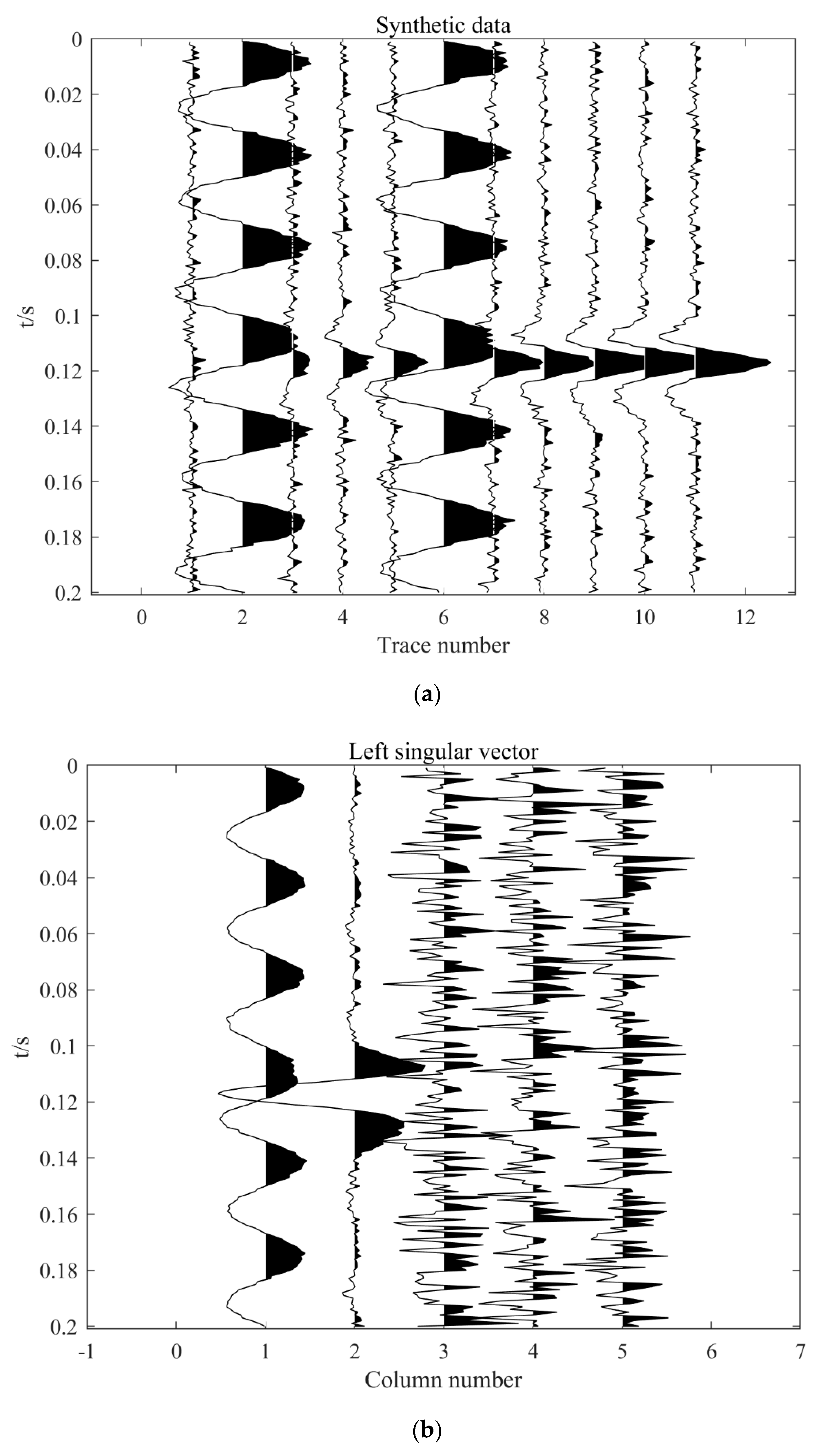
Figure 1. (a) Synthetic data; (b) the left singular vector diagram corresponding to the effective signal after SVD; (c) the right singular vector diagram corresponding to the effective signal.
Applsci 12 12840 g001aApplsci 12 12840 g001b
Figure 2. Improved SVD process for seismic data.
Applsci 12 12840 g002
Figure 3. MobileNetV2 network architecture.
Applsci 12 12840 g003
Figure 4. The general construction of the bottleneck layer of the MobileNetV2 network, referenced from [23].
Applsci 12 12840 g004
Figure 5. Convergence speed of MobileNetV2 during the training process.
Applsci 12 12840 g005
Figure 6. The trained MobilenetV2 network can predict the six right singular vectors as (af), respectively.
Applsci 12 12840 g006
Figure 7. (a) Synthetic seismic data without noise; (b) seismic data with noise added.
Applsci 12 12840 g007
Figure 8. Filtered results were achieved using conventional SVD filtering with (a) K = 1 and (b) K = 2; (c) improved SVD filtering.
Applsci 12 12840 g008aApplsci 12 12840 g008b
Figure 9. (a) Original field seismic data; filtered results achieved using conventional SVD filtering with (b) K = 1 and (c) K = 2; (d) improved SVD filtering.
Applsci 12 12840 g009aApplsci 12 12840 g009bApplsci 12 12840 g009c
Figure 10. (a) Original field seismic data; filtered results achieved using conventional SVD filtering with (b) K = 1 and (c) K = 2; (d) improved SVD filtering.
Applsci 12 12840 g010aApplsci 12 12840 g010bApplsci 12 12840 g010c
Table 1. MobileNet comparison to popular models.
ModelBatch SizeRun Time (h)ImageNet Accuracy (%)
restnet5088.7799.91
MobileNetV2163.2599.94
Table 2. MobileNetV2 network architecture.
InputNetwork LayerExpansion MultiplierOutput ChannelsNumber RepetitionsStride
224 2   ×   3 conv2d-3212
112 2   ×   32 bottleneck61611
112 2   ×   16 bottleneck62422
56 2   ×   24 bottleneck63232
28 2   ×   32 bottleneck66442
14 2   ×   64 bottleneck69631
14 2   ×   96 bottleneck616032
7 2   ×   160 bottleneck632011
7 2   ×   320 conv2d 1 × 1-128011
7 2   ×   1280 avgpool 7 × 7--1-
1   ×   1   ×   1280 conv2d 1 × 1-k-
Note: Table 2 is referenced from [23].
Table 3. SNR comparison of denoised results from different methods.
MethodSeismic Data with NoiseConventional SVD,K = 1Conventional SVD,K = 2Improved SVD
SNR (dB)−10.2592−6.8822−6.51768.1007
Table 4. SNR comparison of denoised results from different methods.
MethodOriginal DataConventional SVD, K = 1Conventional SVD, K = 2Improved SVD
SNR (dB)11.333618.529716.817365.7588
Publisher’s Note: MDPI stays neutral with regard to jurisdictional claims in published maps and institutional affiliations.