Article

Disaster Precursor Identification and Early Warning of the Lishanyuan Landslide Based on Association Rule Mining

1
Geophysical and Geochemical Survey Institute of Hunan Province, Changsha 410014, China
2
Key Laboratory of Metallogenic Prediction of Nonferrous Metals and Geological Environment Monitoring (Ministry of Education), School of Geosciences and Info-Physics, Central South University, Changsha 410083, China
3
Hunan Key Laboratory of Nonferrous Resources and Geological Hazards Exploration, Changsha 410083, China
*
Author to whom correspondence should be addressed.
Appl. Sci. 2022, 12(24), 12836; https://doi.org/10.3390/app122412836
Submission received: 9 November 2022 / Revised: 12 December 2022 / Accepted: 12 December 2022 / Published: 14 December 2022

Abstract

:
It is the core prerequisite of landslide warning to mine short-term deformation patterns and extract disaster precursors from real-time and multi-source monitoring data. This study used the sliding window method and gray relation analysis to obtain features from multi-source, real-time monitoring data of the Lishanyuan landslide in Hunan Province, China. Then, the k-means algorithm with particle swarm optimization was used for clustering. Finally, the Apriori algorithm is used to mine strong association rules between the high-speed deformation process and rainfall features of this landslide to obtain short-term deformation patterns and precursors of the disaster. The data mining results show that the landslide has a high-speed deformation probability of more than 80% when rainfall occurs within 24 h and the cumulative rainfall is greater than 130.60 mm within 7 days. It is of great significance to extract the short-term deformation pattern of landslides by data mining technology to improve the accuracy and reliability of early warning.

1. Introduction

Mountains and hills make up more than 60% of the total area of Hunan province in China, half of which have slopes greater than 25° [1]. This area has high rainfall, so landslide disasters are frequent. According to statistics, 2449 various geological disasters occurred in Hunan Province in 2020, causing economic losses of 262.49 million RMB, of which 2116 were landslide disasters, accounting for 86.4% [2]. Deploying multiple types of sensors on landslides to gather information on deformation, rainfall, stress, and other physical parameters, and providing timely warning, are low-cost and reliable prevention methods that can effectively reduce casualties [3,4,5]. With the development of sensor technology and Internet of Things technology, landslide monitoring is gradually developing towards the direction of automation and intelligence [6,7,8,9]. It is of great significance to fully mine extensive monitoring data and extract and identify warning precursors for studying the mechanisms of landslide disasters and improving the accuracy of warning.
Early and accurate identification of landslide precursors is a prerequisite for early warning. The traditional precursors that can be used for early warning are mainly macroscopic phenomena such as surface cracks, slope toe uplift and other macro phenomena [10,11,12]. With the development of monitoring technology, landslide precursors can be mined from abundant monitoring data, of which the most widely used type of data is surface deformation. The accelerated deformation process of landslides is the most intuitive and reliable precursor, so it is widely used in the study of landslide early warning. Xu et al. [5,13] proposed to use the normalized tangent angle as an indicator for early warning of landslides. Jeng et al. [14] proposed to use displacement-velocity ratio as an indicator for landslide warning. Valletta et al. [15] proposed a multicriteria approach to identify accelerated deformation processes in landslides. Bai et al. [16] proposed a hybrid warning algorithm that could identify the landslide acceleration process quickly, automatically, and accurately in an online monitoring and warning system, and achieved the balance of warning immediacy, accuracy, and computational resources through different strategies.
Although displacement, as a precursor of landslide disaster, can give early warning quickly and accurately, it also has many shortcomings. First, the current sensors for displacement monitoring are highly susceptible to environmental influences and often generate false alarms during the warning process [16,17,18]. Second, displacement is the result of a combination of multiple factors, both internal and external to the landslide. The acceleration of displacement foreshadows the initiation of the landslide process, and the warning window is very short [19,20,21]. Finally, the use of a single displacement characteristic for early warning does not take into account the impact of external trigger factors such as rainfall, earthquakes, and construction on the disaster, and is therefore necessarily incomplete.
The development of data mining technology in recent years has provided new research ideas for landslide precursor identification. Data mining technology can filter and analyze useful information and important events from massive data to reveal the internal relationships and hidden rules of data, which have been widely used in the commercial [22,23], industrial [24,25], engineering [26,27], medical [28,29,30] and educational [31,32] fields with remarkable effect. The application of data mining techniques in the field of landslides is mainly focused on susceptibility assessment [33,34,35], aiming to analyze landslide instability risk at the regional scale, while there are very few studies on application in specific landslide monitoring. Ma et al. [36,37] first used modern data mining techniques integrating two-step clustering, association rule mining, and decision trees to analyze data from the Majiagou landslide and the Zhujiadian landslide in the Three Gorges reservoir area. These studies not only identified landslide disaster factors but also realized the prediction of displacement evolution, which was the earliest research to carry out data mining for single landslide monitoring. Miao et al. [38] and Guo et al. [39] adopted the same data mining technology to analyze the trigger factors of the Baishuihe landslide and the Shuping landslide in the Three Gorges Reservoir area, and determined the warning threshold. All these studies have fully and comprehensively considered the correlation between multi-source monitoring data and provided causal relationships between different monitoring variables, which are very helpful for the analysis of landslide damage mechanisms and instability patterns. Most of these studies focused on reservoir landslides in the Three Gorges region of China, with monitoring data collected over several years and on a monthly scale. Therefore, these studies were more focused on the long-term deformation patterns of landslides. However, the daily-scale or even hourly-scale short-term deformation patterns of landslides are equally important in landslide early warning studies. Such short-term deformation patterns contain more reliable precursors of landslide disasters than deformation features, which are important for early warning decisions. In addition, these studies all adopted a two-step clustering algorithm, which is a kind of hierarchical clustering and divides clusters through the process of splitting or clustering, so there is no need to determine the number of clusters. However, for the clustering of daily or even hourly monitoring data, we prefer to flexibly adjust the number of clusters. This kind of data is very complex, and human subjective judgment is still needed. At this time, partition clustering represented by k-means is more appropriate.
The purpose of this paper was to mine the short-term deformation patterns of landslides, identify the precursors of landslides, and obtain more reliable early warnings. In this study, the Lishanyuan Landslide in Hunan Province was taken as the case study. First, the sliding window method was used to extract features from the original monitoring data, then the k-means algorithm optimized by particle swarm optimization (PSO) was used to cluster the features and construct the item set, and the Apriori algorithm was finally used to mine the association rules between different features and determine the short-term deformation pattern of landslides according to the given confidence levels to analyze the precursors of landslide disasters and provide early warnings.

2. Methodology

2.1. Overview

The association mining method as shown in Figure 1 was used to mine the association rules between the triggering factors and landslide displacement, which mainly includes three parts: feature engineering, clustering and association rule mining.
In the feature engineering part, for the original multi-source data obtained from landslide monitoring, the sliding window method is used to scan the monitoring data time series of each source. In the scanning process, the 3 σ criterion is first used to eliminate obvious outliers, and then the corresponding features are calculated according to the type of monitoring data, and finally the feature time series data set is formed.
In the clustering part, for the feature time series obtained in the previous part, the PSO-optimized k-means algorithm is first used for clustering, and then the time series are transformed into item sets, and finally the time series of all features are processed in the same way to build the transaction database.
In the association rule mining part, for the transaction database constructed in the previous section, the Apriori algorithm is used to mine the frequent item sets and association rules in the transaction database and analyze the disaster factors and destabilization precursors of landslides accordingly.

2.2. PSO-Optimized k-Means Algorithm

The original value-based monitoring dataset must be changed into a category-based transactional database since the Apriori algorithm for association rule mining is category-based. The k-means algorithm is the most well-known clustering algorithm, whose core objective is to classify the dataset into K clusters, with the elements in each cluster having a high degree of similarity. The k-means algorithm is simple to implement and fast to cluster, but it is very sensitive to the choice of initial cluster centers. Different initial values may lead to different clustering results, i.e., local optima rather than global optima. To solve this problem, we used the PSO algorithm for global optimization. The PSO algorithm is an evolutionary algorithm based on population intelligence that finds the optimal solution by simulating the process of a flock of birds searching for food. The specific steps of the k-means clustering algorithm optimized by PSO are as follows:
Step 1: Particle swarm initialization. Suppose there is a particle swarm composed of m particles in a given D-dimensional search space, and each particle has only two attributes: position and velocity, where position is the code of the solution to be solved and the velocity is the iteration step size.
For the i t h particle, its coordinate position can be expressed as:
X i   =   x i 1 , x i 2 , , x i D
The velocity of the i t h particle can be expressed as:
V i   =   υ i 1 , υ i 2 , , υ i D
When performing k-means clustering on the dataset D   =   x 1 , x 2 , , x n , the initial cluster centers C   =   μ 1 , μ 2 , , μ k need to be specified. In order to avoid the problem of local optimal clustering caused by the sensitivity of C , we coded C as X i in Equation (1) for global optimization.
Step 2: Particle clustering and fitness calculation. Perform k-means clustering after decoding each particle in the particle swarm. The specific steps are as follows:
Sub-step 2.1: For each element x i in the dataset D , the Euclidean distance d i j   =   i = 1 n x i μ j 2 between x i and the center μ j of each cluster is calculated and the current element x i is assigned to the cluster C j represented by the center with the smallest distance.
Sub-step 2.2: For each cluster C j obtained in Sub-step 2.1, the central μ j   =   1 C j x C j x of that cluster is recalculated and the C   =   μ 1 , μ 2 , , μ k is updated.
Sub-step 2.3: Repeat the sub-step 2.1 and 2.2 until the center μ j and element x i of each cluster C j no longer change. Then, the final clustering result can be obtained.
Sub-step 2.4: To evaluate the clustering effect of the current position of each particle, the following equation is used to calculate the fitness F ( i ) of each particle.
F ( i )   =   i = 1 n j = 1 k x i μ j 2
where x i denotes the i t h element in the dataset, and μ j is the center of the i t h cluster. The fitness function represents the sum of the squares of the distances between each element and the center of the cluster to which the element belongs, and the smaller the fitness, the better the clustering effect. The individual optimal solution P i and the group optimal solution g b e s t can be obtained through fitness.
The optimal position searched by the i t h particle is denoted as:
P i   =   p i 1 , p i 2 , , p i D
The optimal position searched by the particle swarm is denoted as:
g b e s t   =   g 1 , g 2 , , g D
Step 3: Position update. Update the position and velocity of each particle with the following equation:
V i k + 1   =   ω V i k   +   c 1 r 1 P i k X i k   +   c 2 r 2 g b e s t k X i k
X i k + 1   =   X i k   +   V i k + 1
where V i k denotes the velocity of the i t h particle at the k t h iteration. X i k denotes the position of the i t h particle at the k t h iteration. P i k denotes the individual optimal solution of the i t h particle up to the k t h iteration. g b e s t k denotes the population optimal solution of the particle swarm as of the k t h iteration. c 1 and c 2 denote the acceleration constants to adjust the step size. r 1 and r 2 denote the random numbers between 0 and 1, respectively, to enhance the randomness of the search process.
Step 4: After the velocity and position of each particle are updated, the particles that are out of the solution range are initialized randomly again. If the current fitness function value is better than the historical optimal P i , then update P i . Similarly, if the population fitness function value of the updated particle population is better than the historical optimal g b e s t , then update g b e s t .
Step 5: Repeat Step 2 to 4, and constantly update and iterate for all particles until the maximum number of solutions is reached or the aggregation degree σ 2 of the group optimal solution g b e s t is less than the given threshold.
σ 2   =   1 n i = 1 n F ( i ) F ¯ 2
where F ¯ is the average fitness of the particle swarm, and σ 2 represents the aggregation degree of the particles in the particle swarm. The smaller its value, the higher the convergence degree of the PSO algorithm. When σ 2 is less than the given threshold, this means that the particles are all clustered near the global solution. At this time, the particle with the best fitness is the initial center of the global optimal clustering, and the clustering result can be obtained using k-means for clustering.

2.3. Association Rule Mining and Apriori Algorithm

Association rule mining refers to the discovery of valuable correlation information and knowledge rules from data sets. The Apriori algorithm is the most classic algorithm for mining association rules. Suppose I   =   i 1 , i 2 , , i m is an item set, each element i m of which is called an item, and the item set of length k is called k i t e m s e t . A subset of item set I can form a transaction, and multiple transactions can form a transaction database T   =   t 1 , t 2 , , t n . Suppose X and Y are two item sets in the transaction database whose intersection is empty, that is, X T , Y T and X Y = . These two item sets can be denoted by X Y and if there is an association rule the former item X denotes the condition of the association rule and the latter item Y denotes the conclusion of the association rule. To better measure the performance of the mined association rules, three indicators need to be used: support, confidence and lift. Their definitions are as follows:
Support is the probability that X and Y occur together in the transaction database T . Support indicates the importance of association rule X Y in the total data:
S X Y   =   T X Y T
Confidence is the probability that Y will occur if X is included. Confidence expresses the validity of the association rule X Y :
C X Y   =   T X Y T X
Lift is the ratio of the confidence to the occurrence probability of the later term Y in the transaction database T . Lift indicates the strength of the correlation, and the larger the lift, the stronger the correlation:
L X Y   =   T X Y T X / T Y T
where T X Y represents the number of item sets X and Y appearing in the transaction database T at the same time. T represents the number of transactions in the transaction database T . T X and T Y represent the number of item sets X or Y appearing in the transaction database T , respectively.
The minimum support m i n _ s u p p and minimum confidence m i n _ c o n f need to be specified as thresholds in association rule mining. If the support of an item set is greater than m i n _ s u p p , then this item set is called frequent item set. If the support and confidence of an association rule are greater than the m i n _ s u p p and m i n _ c o n f , then this rule is called a strong association rule. The specific flow of the Apriori algorithm is shown in Figure 1 and described in detail as follows:
Step 1: Iterate through all the transactions in the transaction database T and count the number of each item and calculate the support. The items with the support greater than m i n _ s u p p are deleted to generate the frequent 1-item set L 1 .
Step 2: Generate candidate 2-item set for L 1 by joining and pruning operations, calculate the support of each item in the candidate 2-item set and also filter according to the m i n _ s u p p to get the frequent 2-item set L 2 . Repeat this process until the candidate k i t e m s e t is empty, thus obtaining the frequent k i t e m s e t .
Step 3: Calculate the confidence of each L k separately, and output the association rules with confidence greater than m i n _ c o n f .

3. Study Area

3.1. Landslide Overview

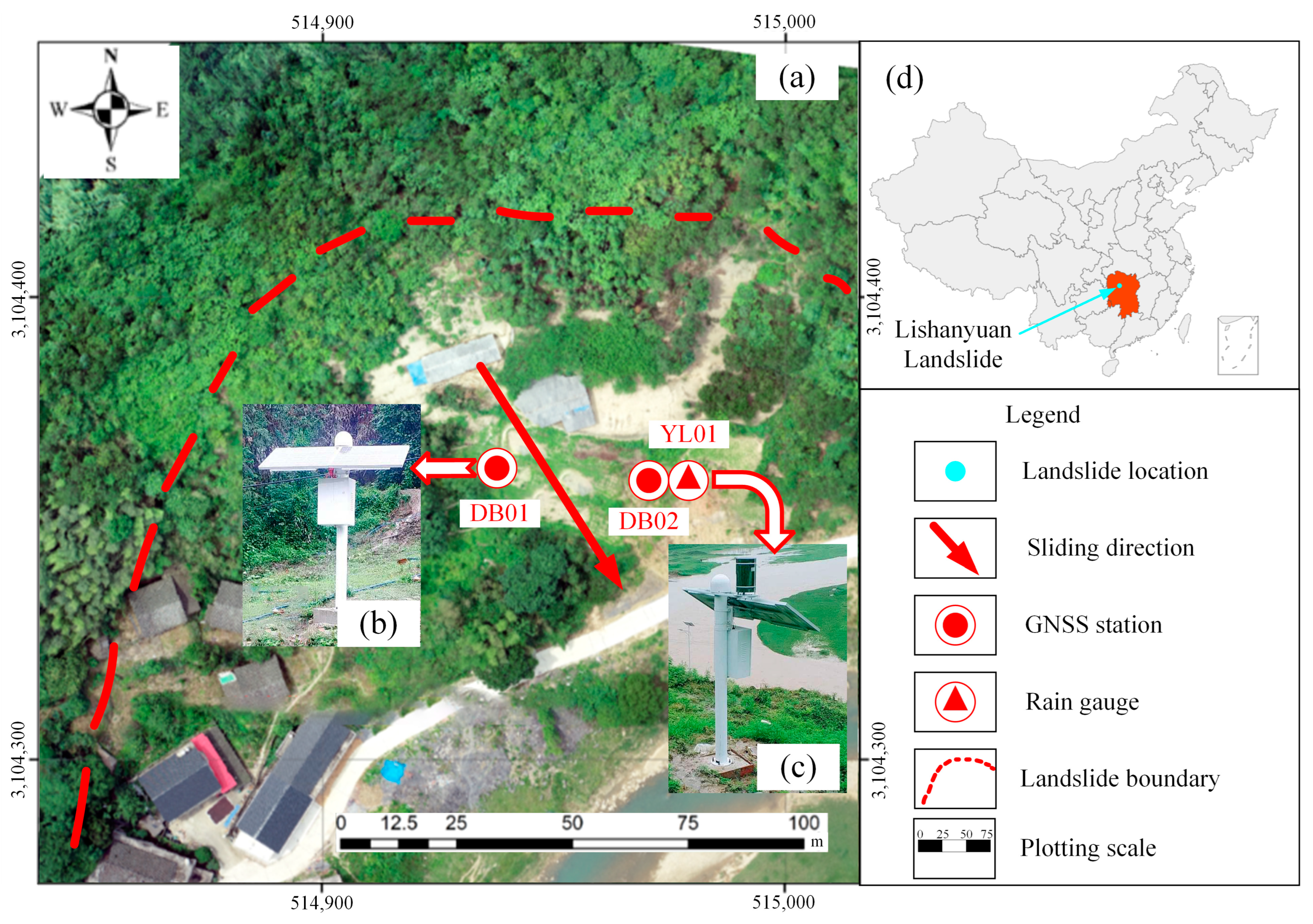
The Lishanyuan landslide is located in Xinhua County, Hunan Province, China (Figure 2). The longitudinal length of the landslide is 120 m, the horizontal width is 300 m, the average thickness is about 3 m, and the total volume is about 1.08 × 10⁵ m3. The landslide is a shallow landslide with a main slide direction of 210°. The middle and back edges of the slope are well covered with vegetation. There are several residential houses at the left foot of the slope. The area on the right side of the slope is poorly covered with vegetation. There is a village-level road and a small stream at the front edge of the landslide, and the foot of the slope has been washed by the river for a long time. Due to long-term river scouring at the foot of the slope, the landslide initially showed accelerated deformation characteristics in 1996. From then until 2012, it underwent a slow deformation trend. In 2013, the landslide accelerated again, with multiple cracks on the slope and subsidence of the village-level road. In April 2018, affected by heavy rainfall, the landslide had a local slip of about 600 m3, and the sliding soil fell to the walls and windows of residential houses on the lower side of the slope, causing a direct loss of about 600,000 RMB. According to the on-site investigation, the landslide is a small and shallow traction landslide, which is very common and representative in Hunan Province, China.

3.2. Deformation Characteristics

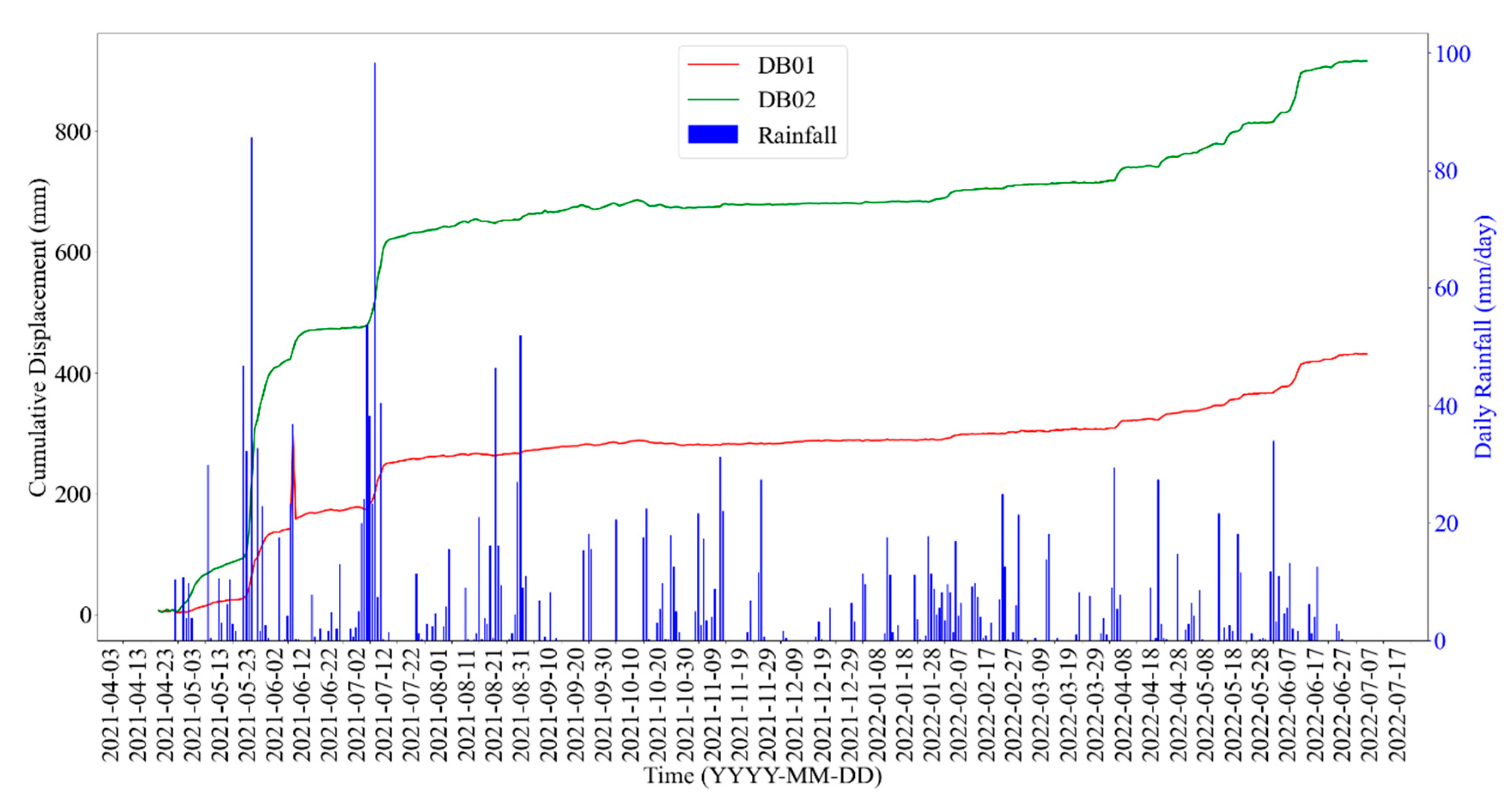
To protect the safety of the residents below the landslide, we completed the deployment and commissioning of monitoring equipment to establish a monitoring and early warning system on 15 April 2021. The location and photos of the monitoring stations are shown in Figure 2. Two GNSS monitoring stations, named DB01 and DB02, were deployed on the main slide profile of the landslide, and the GNSS base stations are located on the roadside of the lower side of the landslide. In addition, a rain gauge named YL01 was deployed at DB02. The automated monitoring system received the first monitoring data at 17:00 on 15 April, and the default acquisition interval of the GNSS monitoring stations was 1 h. As the landslide appeared to accelerate significantly on 17 May, the GNSS monitoring stations adjusted the collection interval to 30 min, and the collection interval of the rain gauge was adjusted to 20 min. As of 15:00 p.m. on 1 July 2022, a total of 57,597 monitoring data were collected by the monitoring system, including 30,396 GNSS monitoring data and 27,201 rainfall monitoring data. The monitoring data are shown in Figure 3.
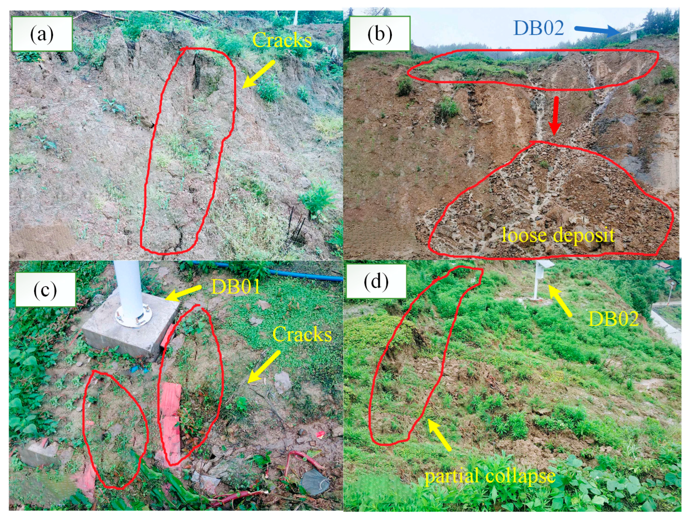
From Figure 3, it can be seen that the deformation patterns of the two GNSS monitoring stations are basically the same, but the deformation amplitude of DB02 is significantly larger than that of DB01, which indicates that the deformation of the leading edge of this landslide is larger than that of the trailing edge of the landslide, which is consistent with the deformation characteristics of the traction landslide. The threshold design and warning process of this landslide are described in Bai et al. [16] The deployed monitoring and warning system is able to accurately and quickly identify the accelerated deformation process of the landslide and report timely warnings. To verify the reliability of the monitoring data, we inspected the landslide site on 19 May 2021. At this time, the landslide area had just experienced a strong rainfall, and the monitoring data from two GNSS monitoring stations showed that the landslide had been violently deformed. We found multiple cracks in the landslide body during a site inspection (Figure 4), obvious slippage, soil accumulation at the foot of the slope, and small mudslides in the local area. These macroscopic phenomena are consistent with the monitoring and early warning results, proving the effectiveness and reliability of the monitoring and early warning system.
The deformation process of Lishanyuan landslide shows obvious correlation with the rainfall process. Taking the DB02 monitoring station with the most obvious deformation as an example, the displacement of the two GNSS monitoring stations first showed a fluctuation of 10 mm for about a week after the monitoring started, indicating that the measurement accuracy of GNSS was of centimeter level. Affected by the rainfall event on 22 April 2021, the acceleration process began with the synchronization of the displacements of the two GNSS monitoring stations starting at 4:00 a.m. on 23 April. After that, the displacements of the two monitoring stations showed a step-like growth, and each severe deformation process was accompanied by concentrated high-intensity rainfall. After mid-October, the rainfall decreased, and the deformation began to slow down, showing creep characteristics. After April of the following year, the landslides started a process of obvious deformation and acceleration again.

3.3. Feature Engineering

From the deformation characteristics reflected by the Lishanyuan landslide monitoring data, we found that the deformation process of the landslide showed an obvious correlation with the rainfall process. To further mine the association rules of this correlation, we needed to carry out further data mining on the monitoring data, for which feature engineering was first needed. Feature engineering refers to extracting more representative features from raw monitoring data to improve the effectiveness of mining tasks. For the monitoring data and deformation characteristics of the Lishanyuan landslide, we constructed features for both deformation and velocity. In terms of deformation, we focused more on the accelerated deformation process, so the deformation velocity was the most important feature. The deformation velocity ( υ D B 01 , υ D B 02 ) of two GNSS monitoring stations was chosen as the main feature. In terms of rainfall, we paid attention not only to the short-term rainfall features, but also to the long-term rainfall features. We chose the cumulative rainfall of three hours q 3 h , six hours q 6 h , twelve hours q 12 h , 24 h q 24 h , three days q 3 d , and seven days q 7 d as the characteristics reflecting rainfall.
According to Bai et al. [40] and Liu et al. [41], the strength of correlation between features can be quantitatively determined by gray relation analysis. Therefore, we used the gray relation analysis algorithm to calculate the gray relation degree between various types of rainfall features and deformation velocity; the calculation results are shown in Table 1. From Table 1, we can see that the gray relation degree of all rainfall features and deformation velocity is greater than 0.9, which is much higher than the empirical threshold of 0.6. So, all of these rainfall features can be adopted.

4. Results

4.1. Clustering Results

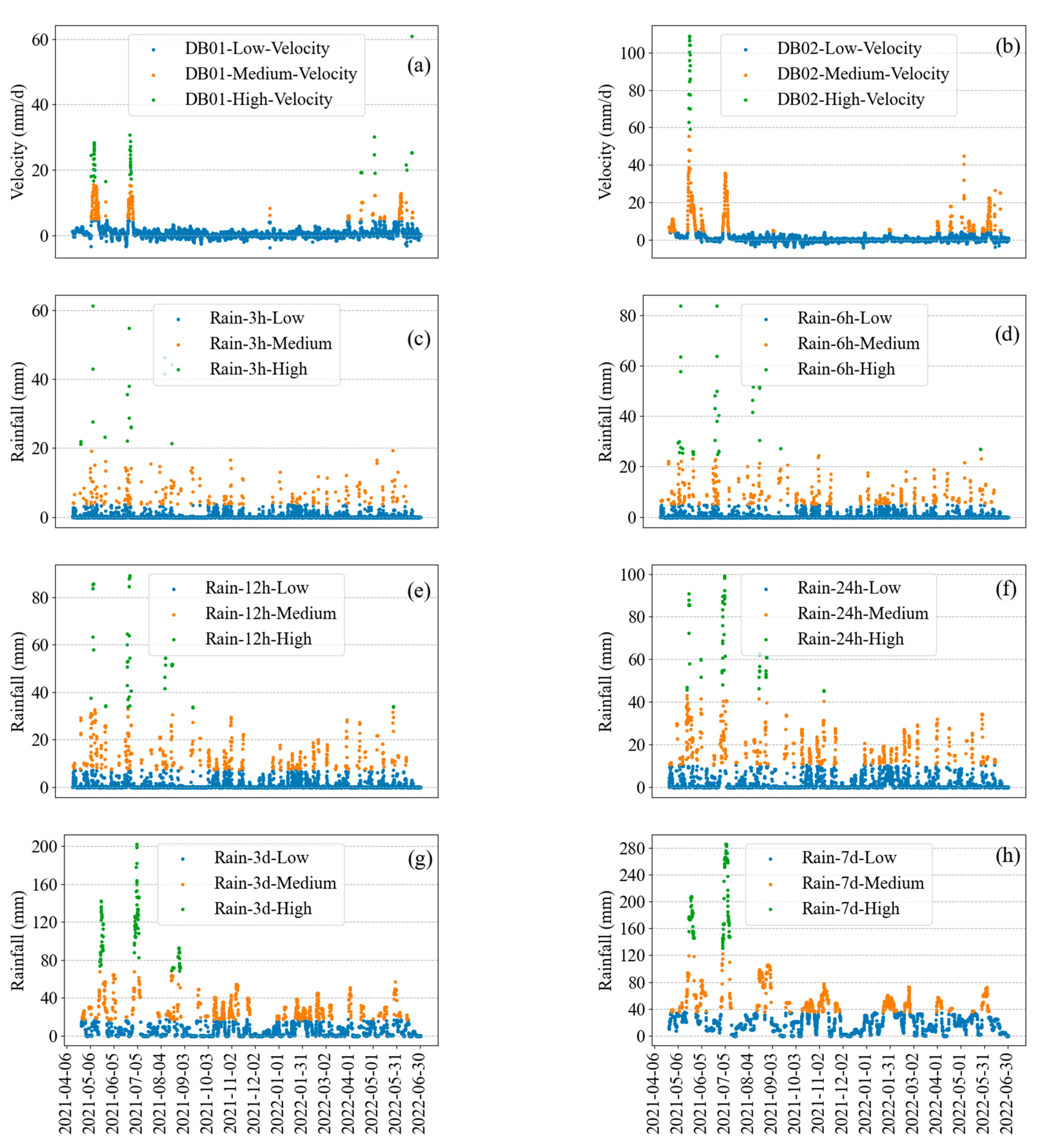
For the various types of feature sequences obtained from feature engineering, we used the PSO-optimized k-means algorithm to cluster each feature. The number of cluster centers for each type of feature was set to 3, thereby clustering the feature into low, medium, and high clusters. The clustering results of all features are shown in Figure 5, and the interval ranges and sample sizes of different clusters are shown in Table 2.
Combining Figure 5 and Table 2, it can be seen that the number of samples in different clusters differs by an order of magnitude. The number of samples of low-rank clusters is much higher than that of middle-rank and high-rank clusters, and the number of samples of middle-rank clusters is also much higher than that of high-rank clusters. Combining Figure 5 and Table 2, it can be seen that the number of samples in different clusters differs by an order of magnitude. The number of samples of low-rank clusters is much higher than that of middle-rank and high-rank clusters, and the number of samples of middle-rank clusters is also much higher than that of high-rank clusters. Taking υ D B 01 as an example, the speed of samples in the DB01-Low-Velocity cluster is between −3.64 and 4.70, which has a total of 4887 samples. The speed of samples in the DB01-Medium-Velocity cluster is between 4.78 and 15.54 with a total of 253 samples, which is an order of magnitude less than the DB01-Low-Velocity cluster. The speed of samples in the DB01-High-Velocity cluster is between 16.49 and 60.96, and the number of samples is only 56, which is an order of magnitude less than the DB01-Medium-Velocity cluster. The clustering results of other features have similar characteristics to υ D B 01 , differing only in the range of intervals. The boundaries between the different clusters are very clear, and the characterized velocities or intensities of rainfall are largely consistent with the actual situation.

4.2. Association Rule Mining Results

After clustering, each cluster is named, and then the values in the features converted into category names. The category names of different features at each moment form an item set, thereby transforming the entire feature dataset into a transaction database. The Apriori algorithm was used to carry out the association rule mining study on this transaction database to mine strong association rules between rainfall features and the velocities of two GNSS monitoring stations separately. We took the velocity of GNSS monitoring stations as the latter term and the rainfall characteristics as the former term, and obtained the corresponding strong association rules based on both different m i n _ c o n f and m i n _ s u p p . For the velocity of the DB01 monitoring station, we set the m i n _ s u p p as 0.3% and the m i n _ c o n f as 80%. For landslide warning, we focused more on the high-speed deformation process, which is the DB01-High-Velocity cluster, so we filtered the eligible association rules as shown in Table 3.
For the velocity of DB02 monitoring station, we set the m i n _ s u p p as 0.1% and the m i n _ c o n f as 80%. We also filtered the association rules with DB01-High-Velocity as the latter term in the same way (see Table 3).
A lot of interesting information can be obtained from the association rules in Table 3. First, the lift of all these association rules is much greater than 1, indicating that the presence of rainfall former terms in these association rules has a significant positive effect on the high-speed deformation of landslides. Second, if the rainfall characteristics are classified into the current moment (3 h, 6 h), short-term (12 h, 24 h), and long-term (3 days, 7 days), then the recent rainfall characteristics are not significant in the association rules. For example, in Rules 3–8 and 11–16, these association rules with recent rainfall characteristics can be considered as subordinate rules of the four main rules: Rule 1, Rule 2, Rule 9, and Rule 10. Third, from the four main rules of Rule 1, Rule 2, Rule 9, and Rule 10, the high-speed deformation of landslides requires not only the occurrence of short-term rainfall characteristics, but also long-term rainfall characteristics, and the occurrence of only one of them does not induce the high-speed deformation process of landslides. Fourth, for the DB01 monitoring station, the long-term heavy rainfall characteristics are more important for high-speed deformation of the landslide, because the three-day or seven-day rainfall characteristics in Rule 1–8 are heavy rainfall, and the 12- and 24-h rainfall characteristics can be low-intensity rainfall. Fifth, for the DB02 monitoring station, not only the long-term heavy rainfall characteristics of 3–7 days but also the short-term heavy rainfall characteristics of 24 h are required.
In conclusion, by analyzing the monitoring data of the Lishanyuan landslide, it can be initially concluded that the landslide is caused by rainfall. Through association rule mining, the disaster factors can be more accurately identified as the combination of short-term rainfall and long-term heavy rainfall. When making early warning decisions, a rainfall within 24 h and a heavy rainfall with a cumulative rainfall greater than 130.60 mm within 7 days can be used as a precursor to identify the high-speed deformation of the landslide.

5. Discussion

To analyze the disaster factors of the Lishanyuan landslide and determine the precursors of high-speed deformation of the landslide, we used a combination of PSO-optimized k-means clustering algorithm and the Apriori algorithm to mine the association rules of the monitoring data. The analysis results of the mined strong association rules show that the high-speed deformation process of the Lishanyuan landslide is mainly affected by the combination of short-term rainfall of about 1 day, and long-term heavy rainfall of about 3–7 days. A rainfall within 24 h and a heavy rainfall with a cumulative rainfall greater than 130.60 mm within 7 days can be used as a precursor to identify the high-speed deformation of the landslide. Such a precursor can improve the ability of warning.
The association rule mining algorithm used in this study has the following main advantage. First, we used the sliding window method to extract features in the feature engineering part. This method improves the data utilization by considering continuous data over a period of time comprehensively, compared to considering only the features at the current moment, thus improving the reliability and representativeness of the obtained features. Second, the original k-means clustering algorithm is optimized by using the PSO algorithm, which effectively prevents the clustering results from falling into a local optimal. Third, the k-means algorithm is simple to implement and only requires a given number of clusters, which is easy to quantify. Other clustering methods that do not require specifying the number of clusters often require specifying other hyperparameters that are difficult to quantify. It is more convenient to directly specify the number of clusters for the control of clustering results. Finally, this study is based on real-time monitoring data, whose sampling intervals are hourly or even on the minute scale. Compared with ultra-long-term monitoring data at the monthly scale, it is richer and pays more attention to short-term deformation patterns of landslides, which is of great significance for early warning.
Additionally, it should be noted that our improvement of the association rule mining method results in an increase in algorithm complexity. On the one hand, we use the PSO algorithm to optimize the k-means clustering process, which is an evolutionary algorithm that requires uninterrupted iterative computation of many potential solutions, which is very complex and time-consuming. On the other hand, the Apriori algorithm for mining association rules needs to scan the entire transaction database when processing frequent candidate sets, which has high algorithm complexity, a huge amount of calculation, and is very time-consuming. With the improvement of technology and the passage of monitoring time, the number of monitored landslides and the volume of data will also increase sharply in the future. It is an inevitable trend to explore simple and fast data mining algorithms.
In this study, the Apriori algorithm was used to mine association rules. Therefore, the numerical dataset was converted into a category-type transaction database. This method cannot further quantify association rules and is easily affected by clustering results. Meanwhile, the Apriori algorithm does not consider the time series characteristics of item sets in the mining process of association rules, which results in ignoring the influence of sequence pattern in the mining process. Future research needs to explore a data mining method that uses numerical datasets and considers sequential patterns in order to mine more valuable information.

6. Conclusions

For the monitoring data of the Lishanyuan landslide, the sliding window method was used to extract the features, and gray relation analysis was used to screen the features. Then the PSO-optimized k-means algorithm was used to cluster. Finally, the Apriori algorithm was used to mine the strong association rules between deformation speed and rainfall characteristics to analyze the disaster factors of the Lishanyuan landslide and propose the precursors that can be used for early warning. The following conclusions were obtained from this study:
The sliding window method was adopted to achieve feature extraction of high-frequency monitoring data, which can make full use of the data and be more representative. Using PSO-optimized k-means algorithm to cluster feature engineering can effectively avoid the clustering results falling into local optimal. By clustering, the numerical dataset is transformed into transaction database, and the strong association rules can be mined using the Apriori algorithm. This research developed mining of association rules of monitoring data at hourly or even minute scale. Compared with ultra-long-term monitoring data at monthly scale, we should pay more attention to short-term deformation patterns, which are more conducive to short-term real-time early warning.
The results of association rules mining show that the high-speed deformation process of the Lishanyuan landslide is mainly affected by the combination of short-term rainfall of about 1 day and long-term heavy rainfall of about 3–7 days. A rainfall within 24 h and heavy rainfall with a cumulative rainfall greater than 130.60 mm within 7 days can be used as a precursor to identify the high-speed deformation of the landslide.
The association rule mining algorithm used in this paper is highly complex, computationally intensive, and very time-consuming, and simpler and faster algorithms need to be explored in the future to cope with monitoring and early warning of more and more landslides. In addition, this mining process does not consider the time-series characteristics of item sets, and future research should explore sequence pattern mining, which has uncovered more and more valuable information.

Author Contributions

Conceptualization, J.X., D.B.; methodology, J.X., D.B.; software, J.X., D.B.; validation, J.X. and J.L.; formal analysis, J.X.; investigation, J.X.; resources, J.X. and H.H.; data curation, J.X.; writing—original draft preparation, J.X.; writing—review and editing, J.X., H.H., J.L., D.B., G.L.; visualization, D.B. and J.X.; supervision, J.X.; project administration, J.X.; funding acquisition, G.L. All authors have read and agreed to the published version of the manuscript.

Funding

This research was funded by Key research and development program of Hunan Province of China, grant number: 2020SK2135. Natural Resources Research Project in Hunan Province of China, grant number: 2021-15.

Institutional Review Board Statement

Not applicable.

Informed Consent Statement

Not applicable.

Data Availability Statement

Not applicable.

Acknowledgments

We would like to thank the editor and the reviewers for helping us improve the quality of the manuscript.

Conflicts of Interest

The authors declare no conflict of interest.

References

  1. Yu, D.; Hu, S.; Tong, L.; Xia, C. Spatiotemporal Dynamics of Cultivated Land and Its Influences on Grain Production Potential in Hunan Province, China. Land 2020, 9, 510. [Google Scholar] [CrossRef]
  2. National Bureau of Statistics of the People’s Republic of China. China Statistical Yearbook-2021; China Statistics Press: Beijing, China, 2021.
  3. Bai, D.; Tang, J.; Lu, G.; Zhu, Z.; Liu, T.; Fang, J. The Design and Application of Landslide Monitoring and Early Warning System Based on Microservice Architecture. Geomat. Nat. Hazards Risk 2020, 11, 928–948. [Google Scholar] [CrossRef]
  4. Chen, M.; Jiang, Q. An Early Warning System Integrating Time-of-Failure Analysis and Alert Procedure for Slope Failures. Eng. Geol. 2020, 272, 105629. [Google Scholar] [CrossRef]
  5. Xu, Q.; Peng, D.; Zhang, S.; Zhu, X.; He, C.; Qi, X.; Zhao, K.; Xiu, D.; Ju, N. Successful Implementations of a Real-Time and Intelligent Early Warning System for Loess Landslides on the Heifangtai Terrace, China. Eng. Geol. 2020, 278, 105817. [Google Scholar] [CrossRef]
  6. Liu, Y.; Tang, G.; Zou, W. Video Monitoring of Landslide Based on Background Subtraction with Gaussian Mixture Model Algorithm. In Proceedings of the 2021 IEEE International Geoscience and Remote Sensing Symposium IGARSS, Brussels, Belgium, 11–16 July 2021; pp. 8432–8435. [Google Scholar]
  7. Lau, Y.M.; Wang, K.L.; Wang, Y.H.; Yiu, W.H.; Ooi, G.H.; Tan, P.S.; Wu, J.; Leung, M.L.; Lui, H.L.; Chen, C.W. Monitoring of Rainfall-Induced Landslides at Songmao and Lushan, Taiwan, Using IoT and Big Data-Based Monitoring System. Landslides 2022, 1–26. [Google Scholar] [CrossRef]
  8. Sheikh, M.R.; Nakata, Y.; Shitano, M.; Kaneko, M. Rainfall-Induced Unstable Slope Monitoring and Early Warning through Tilt Sensors. Soils Found. 2021, 61, 1033–1053. [Google Scholar] [CrossRef]
  9. Liu, C.; Shao, X.; Li, W. Multi-Sensor Observation Fusion Scheme Based on 3D Variational Assimilation for Landslide Monitoring. Geomat. Nat. Hazards Risk 2019, 10, 151–167. [Google Scholar] [CrossRef]
  10. Fan, X.; Xu, Q.; Liu, J.; Subramanian, S.S.; He, C.; Zhu, X.; Zhou, L. Successful Early Warning and Emergency Response of a Disastrous Rockslide in Guizhou Province, China. Landslides 2019, 16, 2445–2457. [Google Scholar] [CrossRef]
  11. Zhu, L.; Deng, Y.; He, S. Characteristics and Failure Mechanism of the 2018 Yanyuan Landslide in Sichuan, China. Landslides 2019, 16, 2433–2444. [Google Scholar] [CrossRef]
  12. Ma, S.; Xu, C.; Xu, X.; He, X.; Qian, H.; Jiao, Q.; Gao, W.; Yang, H.; Cui, Y.; Zhang, P.; et al. Characteristics and Causes of the Landslide on July 23, 2019 in Shuicheng, Guizhou Province, China. Landslides 2020, 17, 1441–1452. [Google Scholar] [CrossRef]
  13. Xu, Q.; Yuan, Y.; Zeng, Y.; Hack, R. Some New Pre-Warning Criteria for Creep Slope Failure. Sci. China Technol. Sci. 2011, 54, 210–220. [Google Scholar] [CrossRef]
  14. Jeng, C.J.; Chen, S.S.; Tseng, C.H. A Case Study on the Slope Displacement Criterion at the Critical Accelerated Stage Triggered by Rainfall and Long-Term Creep Behavior. Nat. Hazards 2022, 112, 2277–2312. [Google Scholar] [CrossRef]
  15. Valletta, A.; Carri, A.; Segalini, A. Definition and Application of a Multi-Criteria Algorithm to Identify Landslide Acceleration Phases. Georisk Assess. Manag. Risk Eng. Syst. Geohazards 2021, 16, 555–569. [Google Scholar] [CrossRef]
  16. Bai, D.; Lu, G.; Zhu, Z.; Zhu, X.; Tao, C.; Fang, J. A Hybrid Early Warning Method for the Landslide Acceleration Process Based on Automated Monitoring Data. Appl. Sci. 2022, 12, 6478. [Google Scholar] [CrossRef]
  17. Tan, Q.; Wang, P.; Hu, J.; Zhou, P.; Bai, M.; Hu, J. The Application of Multi-Sensor Target Tracking and Fusion Technology to the Comprehensive Early Warning Information Extraction of Landslide Multi-Point Monitoring Data. Measurement 2020, 166, 108044. [Google Scholar] [CrossRef]
  18. Li, W.; Tsung, F.; Song, Z.; Zhang, K.; Xiang, D. Multi-Sensor Based Landslide Monitoring via Transfer Learning. J. Qual. Technol. 2021, 53, 474–487. [Google Scholar] [CrossRef]
  19. Bai, D.; Lu, G.; Zhu, Z.; Zhu, X.; Tao, C.; Fang, J. Using Electrical Resistivity Tomography to Monitor the Evolution of Landslides’ Safety Factors under Rainfall: A Feasibility Study Based on Numerical Simulation. Remote Sens. 2022, 14, 3592. [Google Scholar] [CrossRef]
  20. Denchik, N.; Gautier, S.; Dupuy, M.; Batiot-Guilhe, C.; Lopez, M.; Léonardi, V.; Geeraert, M.; Henry, G.; Neyens, D.; Coudray, P.; et al. In-Situ Geophysical and Hydro-Geochemical Monitoring to Infer Landslide Dynamics (Pégairolles-de-l’Escalette Landslide, France). Eng. Geol. 2019, 254, 102–112. [Google Scholar] [CrossRef]
  21. Jiang, Y.; Xu, Q.; Lu, Z.; Luo, H.; Liao, L.; Dong, X. Modelling and Predicting Landslide Displacements and Uncertainties by Multiple Machine-Learning Algorithms: Application to Baishuihe Landslide in Three Gorges Reservoir, China. Geomat. Nat. Hazards Risk 2021, 12, 741–762. [Google Scholar] [CrossRef]
  22. Qing, H.; Zheng, G.; Fu, D. Risk Data Analysis of Cross Border E-Commerce Transactions Based on Data Mining. J. Phys. Conf. Ser. 2021, 1744, 032014. [Google Scholar] [CrossRef]
  23. Tornero-Velez, R.; Isaacs, K.; Dionisio, K.; Prince, S.; Laws, H.; Nye, M.; Price, P.S.; Buckley, T.J. Data Mining Approaches for Assessing Chemical Coexposures Using Consumer Product Purchase Data. Risk Anal. 2021, 41, 1716–1735. [Google Scholar] [CrossRef]
  24. Espadinha-Cruz, P.; Godina, R.; Rodrigues, E.M.G. A Review of Data Mining Applications in Semiconductor Manufacturing. Processes 2021, 9, 305. [Google Scholar] [CrossRef]
  25. Dogan, A.; Birant, D. Machine Learning and Data Mining in Manufacturing. Expert Syst. Appl. 2021, 166, 114060. [Google Scholar] [CrossRef]
  26. Liu, W.; Wang, H.; Xi, Z.; Zhang, R.; Huang, X. Physics-Driven Deep Learning Inversion with Application to Magnetotelluric. Remote Sens. 2022, 14, 3218. [Google Scholar] [CrossRef]
  27. Guo, Y.; Cui, Y.; Xie, J.; Luo, Y.; Zhang, P.; Liu, H.; Liu, J. Seepage Detection in Earth-Filled Dam from Self-Potential and Electrical Resistivity Tomography. Eng. Geol. 2022, 306, 106750. [Google Scholar] [CrossRef]
  28. Hua, S.; Liu, Q.; Yin, G.; Guan, X.; Jiang, N.; Zhang, Y. Research on 3D Medical Image Surface Reconstruction Based on Data Mining and Machine Learning. Int. J. Intell. Syst. 2022, 37, 4654–4669. [Google Scholar] [CrossRef]
  29. Ishaq, A.; Sadiq, S.; Umer, M.; Ullah, S.; Mirjalili, S.; Rupapara, V.; Nappi, M. Improving the Prediction of Heart Failure Patients’ Survival Using SMOTE and Effective Data Mining Techniques. IEEE Access 2021, 9, 39707–39716. [Google Scholar] [CrossRef]
  30. Wu, W.-T.; Li, Y.-J.; Feng, A.-Z.; Li, L.; Huang, T.; Xu, A.-D.; Lyu, J. Data Mining in Clinical Big Data: The Frequently Used Databases, Steps, and Methodological Models. Mil. Med. Res. 2021, 8, 44. [Google Scholar] [CrossRef]
  31. Palacios, C.A.; Reyes-Suárez, J.A.; Bearzotti, L.A.; Leiva, V.; Marchant, C. Knowledge Discovery for Higher Education Student Retention Based on Data Mining: Machine Learning Algorithms and Case Study in Chile. Entropy 2021, 23, 485. [Google Scholar] [CrossRef]
  32. Xin, Y. Analyzing the Quality of Business English Teaching Using Multimedia Data Mining. Mob. Inf. Syst. 2021, 2021, e9912460. [Google Scholar] [CrossRef]
  33. Yong, C.; Jinlong, D.; Fei, G.; Bin, T.; Tao, Z.; Hao, F.; Li, W.; Qinghua, Z. Review of Landslide Susceptibility Assessment Based on Knowledge Mapping. Stoch Environ. Res Risk Assess 2022, 36, 2399–2417. [Google Scholar] [CrossRef]
  34. Rafiei Sardooi, E.; Azareh, A.; Mesbahzadeh, T.; Soleimani Sardoo, F.; Parteli, E.J.R.; Pradhan, B. A Hybrid Model Using Data Mining and Multi-Criteria Decision-Making Methods for Landslide Risk Mapping at Golestan Province, Iran. Environ. Earth Sci. 2021, 80, 487. [Google Scholar] [CrossRef]
  35. Vakhshoori, V.; Pourghasemi, H.R.; Zare, M.; Blaschke, T. Landslide Susceptibility Mapping Using GIS-Based Data Mining Algorithms. Water 2019, 11, 2292. [Google Scholar] [CrossRef] [Green Version]
  36. Ma, J.; Tang, H.; Liu, X.; Hu, X.; Sun, M.; Song, Y. Establishment of a Deformation Forecasting Model for a Step-like Landslide Based on Decision Tree C5.0 and Two-Step Cluster Algorithms: A Case Study in the Three Gorges Reservoir Area, China. Landslides 2017, 14, 1275–1281. [Google Scholar] [CrossRef]
  37. Ma, J.; Tang, H.; Hu, X.; Bobet, A.; Zhang, M.; Zhu, T.; Song, Y.; Ez Eldin, M.A.M. Identification of Causal Factors for the Majiagou Landslide Using Modern Data Mining Methods. Landslides 2017, 14, 311–322. [Google Scholar] [CrossRef]
  38. Miao, F.; Wu, Y.; Li, L.; Liao, K.; Xue, Y. Triggering Factors and Threshold Analysis of Baishuihe Landslide Based on the Data Mining Methods. Nat. Hazards 2021, 105, 2677–2696. [Google Scholar] [CrossRef]
  39. Guo, L.; Miao, F.; Zhao, F.; Wu, Y. Data Mining Technology for the Identification and Threshold of Governing Factors of Landslide in the Three Gorges Reservoir Area. Stoch. Environ. Res. Risk Assess 2022, 36, 3997–4012. [Google Scholar] [CrossRef]
  40. Bai, D.; Lu, G.; Zhu, Z.; Tang, J.; Fang, J.; Wen, A. Using Time Series Analysis and Dual-Stage Attention-Based Recurrent Neural Network to Predict Landslide Displacement. Environ. Earth Sci. 2022, 81, 509. [Google Scholar] [CrossRef]
  41. Liu, Q.; Lu, G.; Dong, J. Prediction of Landslide Displacement with Step-like Curve Using Variational Mode Decomposition and Periodic Neural Network. Bull. Eng. Geol. Environ. 2021, 80, 3783–3799. [Google Scholar] [CrossRef]
Figure 1. Flowchart of association rule mining for the Lishanyuan landslide.
Applsci 12 12836 g001
Figure 2. Geographical location and monitoring scheme of Lishanyuan landslide. (a) Site photograph of the Lishanyuan landslide. (b) Geographical location of the Lishanyuan landslide. (c) Photographs of monitoring stations DB02 and YL01. (d) Photograph of the DB01 monitoring station.
Applsci 12 12836 g002
Figure 3. Daily rainfall data and displacement data from two GNSS monitoring stations for the Lishanyuan landslide.
Applsci 12 12836 g003
Figure 4. On-site inspection photos on 19 May 2021. (a) Long cracks on the surface of the landslide. (b) Loose deposit near the DB02 station. (c) Multiple cracks near DB01 station. (d) partial collapse near DB02 station.
Applsci 12 12836 g004
Figure 5. Visualization of all feature clustering results. (a) The velocity of DB01. (b) The velocity of DB02. (c) 3-h cumulative rainfall. (d) 6-h cumulative rainfall. (e) 12-h cumulative rainfall. (f) 24-h cumulative rainfall. (g) 3-day cumulative rainfall. (h) 7-day cumulative rainfall.
Applsci 12 12836 g005
Table 1. Gray relation degree between rainfall characteristics and displacement characteristics.
q3hq6hq12hq24hq3dq7d
υ D B 01 0.9707350.9710450.9719620.9738570.9784780.979868
υ D B 02 0.9646330.9647420.965820.9680610.9735370.975926
Table 2. Interval range and sample size of all feature clustering results.
Feature NameCluster NameLower Bound Upper BoundCountMeanStandard Deviation
υ D B 01 DB01-Low-Velocity−3.644.7048870.46 1.02
DB01-Medium-Velocity4.7815.542539.09 2.83
DB01-High-Velocity16.4960.965623.58 6.25
υ D B 02 DB02-Low-Velocity−3.844.7746690.60 1.23
DB02-Medium-Velocity4.7955.3750713.39 8.55
DB02-High-Velocity59.24108.842090.67 15.85
q 3 h Rain-3 h-Low0.003.6049620.18 0.56
Rain-3 h-Medium3.8019.402177.33 3.43
Rain-3 h-High21.2061.401734.34 12.17
q 6 h Rain-6 h-Low0.005.0048300.32 0.88
Rain-6 h-Medium5.2024.403339.95 4.57
Rain-6 h-High24.8083.803339.42 16.47
q 12 h Rain-12 h-Low0.007.2046560.64 1.48
Rain-12 h-Medium7.4032.8049413.93 6.12
Rain-12 h-High33.4089.204652.80 17.83
q 24 h Rain-24 h-Low0.0010.4044291.39 2.55
Rain-24 h-Medium10.6043.0069819.64 7.76
Rain-24 h-High45.0099.406968.48 17.00
q 3 d Rain-3 d-Low0.0017.2037364.31 5.12
Rain-3 d-Medium17.4068.20128430.46 11.61
Rain-3 d-High68.60202.20176106.48 28.89
q 7 d Rain-7 d-Low0.0035.20355415.46 10.88
Rain-7 d-Medium35.40122.20145055.17 17.47
Rain-7 d-High130.60285.80192197.53 46.03
Table 3. Association rules related to Lishanyuan landslide deformation.
Rule IDMined Association RulesConfidenceSupportLift
1Rain-24 h-Low & Rain-3 d-High & Rain-7 d-High => DB01-High-Velocity 86.36%0.37%80.13
2Rain-12 h-Low & Rain-24 h-Low & Rain-3 d-High & Rain-7 d-High => DB01-High-Velocity 86.36%0.37%80.13
3Rain-24 h-Low & Rain-3 d-High & Rain-3 h-Low & Rain-7 d-High => DB01-High-Velocity 90.48%0.37%83.95
4Rain-24 h-Low & Rain-3 d-High & Rain-6 h-Low & Rain-7 d-High => DB01-High-Velocity 86.36%0.37%80.13
5Rain-12 h-Low & Rain-24 h-Low & Rain-3 d-High & Rain-3 h-Low & Rain-7 d-High => DB01-High-Velocity 90.48%0.37%83.95
6Rain-12 h-Low & Rain-24 h-Low & Rain-3 d-High & Rain-6 h-Low & Rain-7 d-High => DB01-High-Velocity 86.36%0.37%80.13
7Rain-24 h-Low & Rain-3 d-High & Rain-3 h-Low & Rain-6 h-Low & Rain-7 d-High => DB01-High-Velocity 90.48%0.37%83.95
8Rain-12 h-Low & Rain-24 h-Low & Rain-3 d-High & Rain-3 h-Low & Rain-6 h-Low & Rain-7 d-High =>DB01-High-Velocity 90.48%0.37%83.95
9Rain-12 h-Low & Rain-24 h-High & Rain-7 d-High => DB02-High-Velocity 83.33%0.10%216.50
10Rain-12 h-Low & Rain-24 h-High & Rain-3 d-High & Rain-7 d-High => DB02-High-Velocity 83.33%0.10%216.50
11Rain-12 h-Low & Rain-24 h-High & Rain-3 h-Low & Rain-7 d-High => DB02-High-Velocity 83.33%0.10%216.50
12Rain-12 h-Low & Rain-24 h-High & Rain-6 h-Low & Rain-7 d-High => DB02-High-Velocity 83.33%0.10%216.50
13Rain-12 h-Low & Rain-24 h-High & Rain-3 d-High & Rain-3 h-Low & Rain-7 d-High => DB02-High-Velocity 83.33%0.10%216.50
14Rain-12 h-Low & Rain-24 h-High & Rain-3 d-High & Rain-6 h-Low & Rain-7 d-High => DB02-High-Velocity 83.33%0.10%216.50
15Rain-12 h-Low & Rain-24 h-High & Rain-3 h-Low & Rain-6 h-Low & Rain-7 d-High => DB02-High-Velocity 83.33%0.10%216.50
16Rain-12 h-Low & Rain-24 h-High & Rain-3 d-High & Rain-3 h-Low & Rain-6 h-Low & Rain-7 d-High => DB02-High-Velocity 83.33%0.10%216.50
Publisher’s Note: MDPI stays neutral with regard to jurisdictional claims in published maps and institutional affiliations.