A Simple Portable Magnetometer Based on Magnets and Hall-Effect Sensors Capable of Measuring Magnetic Properties

Abstract

A magnetometer based on Hall effect sensors was developed using a 1020 steel base, two magnets (K&J Magnetics, Pipersville, PA, USA), and two Hall effect sensors: MLX-90215 (Melexis Inc., San Jose, CA, USA) and AD-AD22151 (Analog Devices, Inc., Wilmington, MA, USA). Both sensors were assembled on an acrylic support and powered with a 5-volt battery. The readings can be taken using bench multimeters (HP 34401A or Iminipa ET-2042D). The magnetometer records magnetic hysteresis loop and saturation by applying a field of up to 0.33 T at room temperature. The device was tested using magnetic hysteresis data from samples of 99% pure nickel sphere and magnetite microparticles. A dipole magnetic model was used to obtain the moment of the samples. The sensor used for reading the induced magnetic field of the sample AD-AD22151 has a sensitivity can be adjusted from to 110 mV/mT. This device is cheap, versatile, and easy to build, and despite its low accuracy, when compared to commercial equipment, it can be useful in low-budget teaching and research laboratories.

1. Introduction

Currently, research on the magnetic properties of bulk magnetic materials, micro and nanostructures, is an important tool for students in the fields of physics and engineering [1,2,3,4,5]. The hysteresis curves of a magnetic material can contribute to determining its basic fields of applications. In addition, different magnetic properties, such as remanence magnetization, coercivity, saturation magnetization, hysteresis, Curie temperature, magnetic anisotropy, and susceptibility, can be determined from magnetic hysteresis curves, obtained at room temperature (about 297 K) [3,6]. Magnetic materials can also be classified according to their magnetic curves, and, in the case of nanoparticles, the average diameter can also be estimated [7]. The use of devices called magnetometers is the most common technique used to obtain hysteresis curves of magnetic materials. It is responsible for detecting the induced magnetic fields of the material in the presence or absence of an applied magnetic field [1,2,8,9]. Several magnetometers have been developed over the years for different applications and different types of reading systems of sample-induced field, such as the vibrating sample (VSM), perhaps the oldest one [2], the system based on the superconducting quantum interference device (SQUID) [10], magneto-optical Kerr effect (MOKE) [11], and the Hall effect [1,8,9], with different sensitivities and costs. However, most parts of these devices (magnetometers) are high-cost systems, making them unfeasible for low-budget laboratories, academic studies, or teaching laboratories in many universities.

This study presents a very different approach to measuring magnetic samples using low-cost equipment (magnetometer) developed with items normally accessible to most research and teaching laboratories, such as two magnets (K&J Magnetics, model BX8C8), a 5-volt battery or a power system directly from mains, one MLX-90215 sensor (Melexis Inc.), one AD-AD22151 sensor (Analog Devices, Inc.), and bench multimeters (HP 34401A or Iminipa ET-2042D). The first version of this device (magnetometer) was developed and published by Araujo and his collaborators [12]. This magnetometer has the advantage of being quickly assembled and transported, in addition to the possibility of becoming operational and thus accessible to most research laboratories, being ideal for low-budget basic physics teaching laboratories. The core of this equipment is composed of two magnets, a small circuit board, and an acrylic plate, which serves as a support for the sensors and the sample holder. We use a simple theoretical magnetic dipole model to estimate the magnetic moment. Most commercial magnetometers are not accessible to a teaching laboratory other than the proposed equipment. Thinking about it, we use a simple model to characterize the results obtained in the measurements. The magnetometer was tested using commercially purchased bulk and microparticle samples.

2. Magnetometer Design

We developed equipment using only available and inexpensive components. This was an important issue in the design of this system. Figure 1a shows a schematic drawing of the designed magnetometer: (1) We used an acrylic plate of 65 × 55 mm with 10.5 mm of thickness, two Hall effect sensors were attached to them, (2) two neodymium magnets of the same configuration containing 12.78 mm thick and 19 mm in diameter, (3) all these were on an iron base containing two screws of the same configuration, with approximately 30 mm in diameter and 109 in length, (4) a printed circuit board used to operate the sensor plate details can be seen in Figure 1b, (5) an alignment system consisting of a screw and a spring system, necessary to align the probe Hall to improve the detection of the sample induced field, (6) an aluminum base, (7) a battery set or a power supply system that can supply the sensors with 5 V DC—the output readings are taken by a multimeter. The probe is precisely centered between two neodymium magnets (K&J Magnetics), 19 mm diameter and 12.9 mm length. A magnetic field of up to 0.4 T can be detected.

In addition, the homogeneity of the magnetic field applied by the magnets was verified. In this study, we used a 9640 commercial magnetometer (F. W. Bell Inc., Orlando - US). The probe was built using two Hall effect sensors: One MLX-90215 sensor (Melexis Inc.) with an active sensitivity area of 0.20 × 0.20 mm, which has a gain from programming 4.1 to 140 mV/mT, and a voltage that can be adjusted from 0.03 to 4.97 V (this sensor needs to be programmed and calibrated before use), and one AD-AD22151 sensor (Analog Devices, Inc.), which has an active diameter of 300 µm, with sensitivity ranging from 10 to 110 mV/mT. Differently from the first one, this sensor was designed to vary its sensitivity during operation [12,13].

First, we analyzed the behavior of the sensors in the laboratory environment, using a thermocouple connected to one of the magnets. At the position of the Melexis sensor, no temperature change was detected during the measurement period, even when the magnet got closer to the sensor. For better performance, we used a circuit board developed by Araujo and his collaborators (See Figure 1b) [13]. Figure 1b shows the circuit board specifications: R1 is an 18 kΩ resistor, R2 is a 1 kΩ resistor, R3 is a variable resistor from 0 to 10 kΩ (trimmer), C1 and C2 are capacitors, C1 is a 1 µF power filter and C2 has 0.1 µF, 1 to 8 refers to the connection pins of the AD22151 sensor (sensor input and output connections). Furthermore, in the space between the magnets, where there is an acrylic plate, the magnetic field applied nearby the probe has high homogeneity and is suitable for the sample holder sizes. The noise of both sensors was analyzed, and we measured noise of approximately 40 µV, using equipment to analyze the spectrum (SR760 Stanford Research Systems Inc., Culver City, CA, USA).

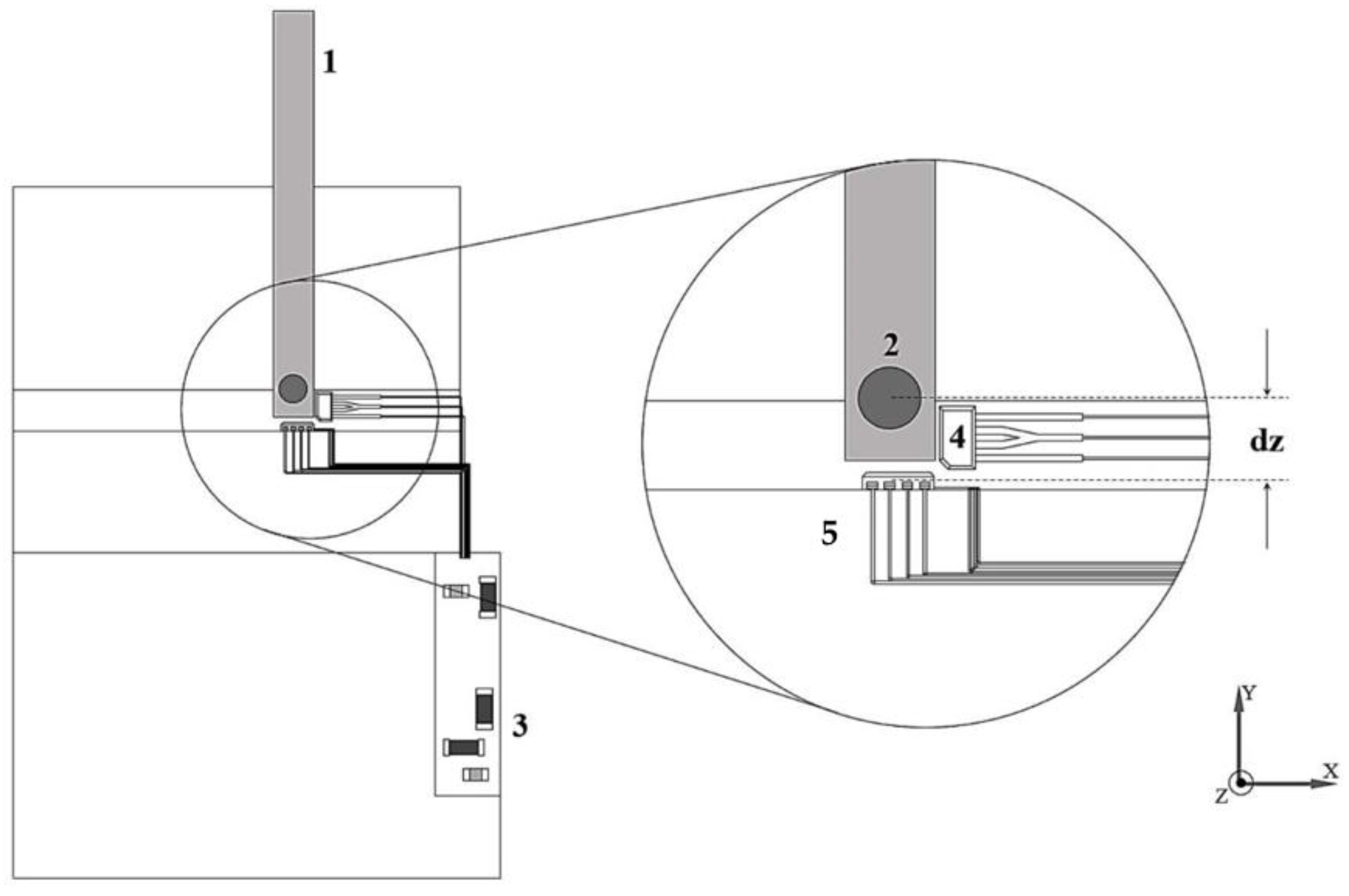
In Figure 2, we can see the probe Hall built on an acrylic structure, with two bands of 56 × 56 mm and 6.4 mm thickness. One of the bands is used to assemble the sensors, and the other for the sample holder. The probe components are: (1) Acrylic sample holder, (2) containing a cylindrical cavity of 3.0 mm diameter and 3.0 mm deep, located near one of the ends–in addition to analyzing fine particles, the sample holder can analyze bulk materials, particles and liquid samples (such as magnetic nanoparticles in oil), (3) S1 sensor circuit board (See Figure 2, No. (5)), AD-AD22151 Hall effect sensor (Analog Devices, Inc.), with variable sensitivity, responsible for detecting the sample induced magnetic field on the y-axis, we can select the sensitivity using a switch attached to the multimeter, (4) S2 MLX-90215 Hall effect sensor (Melexis Inc.), calibrated with a fixed sensitivity of 2.8 mV/mT and an offset of 0.4 V. This sensor is responsible for detecting the magnetic field of magnets in the z-axis. In this assembly, we used two bench multimeters to detect the two sensors: HP 34401A and Iminipa ET-2042D. To power the Hall effect sensors with 5 V, we can use a battery or a power system connected to the mains.

The developed magnetometer can be seen in Figure 3a and all components used can be seen in Figure 3b, as follow: (1) Magnet support base (cylindrical shape) of 30 mm diameter and approximately 109 mm long, (2) aluminum base of 45 × 45 mm and 22 cm length, used as a linear rail, (3) two iron threaded nuts to keep the magnets fixed, bring them closer or move them away from the sample, varying thus the applied magnetic field, (4) fixed iron structure to fix the probe Hall, nuts and alignment screw, (5) device built to activate sensors S1 and S2, this device was connected to a multimeter, (6) probe Hall, (7) cylindrical neodymium magnet of 19 mm diameter and 12.9 mm length, (8) and (9) sample holder, acrylic plates of 5.2 × 3.1 × 32 mm, which is a sample holder that can analyze samples within a cylindrical cavity of 3.0 mm diameter and 3.0 mm length, (10) screw used to align the probe Hall with the magnetic field that can be applied by the magnets, (11) multimeter used for reading Hall sensors.

The AD-AD22151 Hall effect sensor was calibrated to maximum sensitivity (110 mV/mT) Figure 3a. The calibration curve is shown in Figure 4a. In this curve, we can observe that the Hall sensor has a linear relationship with the induced field voltage and the applied magnetic field. We can also observe that there was no hysteresis in the sensor, which is a result typical of the Hall effect sensor. In addition, we analyzed the signal/noise ratio of the AD22151 sensor at the minimum and maximum sensitivities. The curves are shown in Figure 4b. In this figure, we can see that when AD22151 has a noise of approximately 40 µV. These results identify the noise of the magnetometer reading system, the peak of the graph is related to an AC magnetic field applied at 4.0 Hz. Figure 4c represents a theoretical and experimental graph of the behavior of the magnetic field of the magnet in relation to spatial distance in the z axis starting from the center of one of the magnet’s surfaces, the theoretical curve was obtained using the cylindrical model used by Camacho and Sosa [14]. In Figure 4c, we can verify that the experimental results are in agreement with the theoretical curve based on Equation (1) taken from the paper published by Camacho and Sosa [14]. Already in

Table 1. Magnetic field applied by the magnet Bz in Gauss in relation to the distance from the z axis in mm.

Bz (T)	0.46	0.40	0.29	0.19	0.14	0.10	0.08	0.06	0.045	0.041	0.035
z(mm)	0.0	2.0	4.0	6.0	8.0	10	12	14	16	18	20

, we can verify the relationship between the magnetic field applied by the magnet and the distance in the z axis in mm.

$$\mathrm{B}\left(z\right)=\frac{{\mu }_0{m}_z}{2}\left[\frac{z}{\sqrt{z^2+R^2}}-\frac{z-L}{\sqrt{{\left(z-L\right)}^2+R^2}}\right]$$

(1)

3. Calibration and Results

To estimate the magnetization of the material, we need a mathematical model. The simplest is the single magnetic dipole located at the center of the sample. In this case, we should assume that the sample is homogeneous and neglect the fact that we are measuring too close to it. However, this is a first-order estimate [12,13]. The magnetic field induced by a dipole depends on the magnetic moment $\overrightarrow{m}$ and the position in which it is measured $\overrightarrow{r}$ [15]. When locating the origin of the coordinate system in the magnetic dipole, the field generated by it is given by

$$\overrightarrow{B}\left(\overrightarrow{r},\overrightarrow{m}\right)=\frac{{\mu }_0}{4\pi }\left[\frac{3\left(\overrightarrow{m}·\overrightarrow{r}\right)}{r^5}-\frac{\overrightarrow{m}}{r^3}\right]$$

(2)

where μ₀ is the free space permeability. Our configuration applies the magnetic field in the z direction, the detects the x-axis and y-axis components of the response (x₁, y₁, z₁) and m_z represents the magnetic moment only from the z direction, so we are measuring,

$$B_y\left(x_1,y_1,z_1\right)=\frac{{\mu }_0}{4\pi }{m}_z\left[\frac{\left(y_1{z}_1\right)}{{\left(x_1^2+y_1^2+z_1^2\right)}^{5/2}}\right]$$

(3)

Magnetization is the magnetic dipole moment normalized by the mass or volume of the sample. In our case, M_z = $\frac{m_z}{2\pi a^3}$ defined where a is the sample radius.

Therefore, with the help of a handheld microscope (Peak, Inc.) and using the sensor data sheet, we could estimate the relative distances between the center of the sample holder and the active area that lies within the sensor like y₁ = 0.63 ± 0.06 mm and z₁ = 2.30 ± 0.06 mm. We assume that the center of the sphere (3.00 mm diameter) is located in the center of the sample holder, which is the origin of the coordinate system used. Unfortunately, due to the system geometry, we were unable to use the microscope to estimate the position on the x-axis, x₁. Thus, finally, using m_z = 55.25 Am²/kg as the mass magnetization of Ni at 0.4 T [1,8,12,13], we found x₁ = 1.94 mm.

Figure 5 shows the measurements of the sphere in the magnetometer we developed. From this curve, we can estimate some magnetization values for the nickel sphere, close to zero field, as can be seen in Figure 5. These values were compared with the measurements obtained by a commercial magnetometer (MPMS SQUID, Quantum Design Inc., San Diego, CA, USA) in the same sphere. Comparing the two devices (SQUID and PUC-Rio), the average relative error from the farthest point, in relation to the same magnetic field applied, was approximately 38%, whereas in the saturation region, the largest error was only 17% (See

Table 2. Magnetization values in Am²/kg for each applied magnetic field.

Applied Field (T)	0.33	0.32	0.30	0.29
PUC-Rio (Am2/kg)	45.7	44.6	49.2	49.9
SQUID (Am2/kg)	53.9	53.8	53.5	53.58

).

After calibrating the magnetometer, we measured the 99% pure magnetite microparticles, which had been previously purchased. This sample was previously measured using a scanning magnetic microscope, which has a magnetic moment sensitivity of 1.3 × 10⁻¹¹ Am² [16]. To obtain a magnetization curve using this equipment, scanning magnetic maps for each applied magnetic field are necessary. Figure 6 represents magnetic maps of induced magnetic field, we can obtain the magnetic moment, using the point technique developed by Gutierrez and his collaborators [17].

This method consists of obtaining two points in each scanning magnetic map: One with the minimum intensity of the sample-induced magnetic field and another with the maximum intensity. Using a moment that considers the cylindrical cavity of the sample holder, we can obtain the magnetic moment. Afterward, by dividing by the sample mass, we can obtain the magnetization curve (See Figure 6). The scanning magnetic microscope is expensive and has a high cost to be built in most research laboratories because it requires some commercial equipment [16]. In Figure 7a, we can observe the comparison curve between the measurement obtained by our homemade instrument and that obtained in a scanning magnetic microscope. Comparing the two devices (Scanning Magnetic Microscope and PUC-Rio), the average relative error of the most distant point, in relation to the same magnetic field applied, was approximately 39%, whereas in the saturation region, the largest error was only 29%. We believe that these values could be improved if an Arduino board or an acquisition board had been used, such as a National Instruments Board, model NI USB-6008 (See Figure 7b). Thus, more points could be acquired.

The existence of high-resolution magnetometers, which are often expensive equipment, prevents the application of this study in basic physics laboratories. The constituted magnetometer, as well as the theoretical model of a simple dipole, can be a fundamental step for the application of this type of equipment in the teaching of Physics, mainly in the teaching laboratory, since most of the components that make up this equipment are accessible. Feeding in this way, the study of magnetism of materials such as magnetic nanoparticles, microparticles, and even bulk material.

4. Conclusions

We present a magnetometer based on Hall effect sensors of varying sensitivity, which was successfully built and calibrated. This new simple design, using inexpensive components, can be used in low-budget physics and engineering teaching laboratories and is capable of measuring magnetic hysteresis of up to 3.2 kG (0.32 T) at room temperature. The system was tested using a nickel sphere, comparing the measurements with the values obtained in a high-cost commercial magnetometer (SQUID). Although our magnetometer has low sensitivity compared to commercial equipment and no commercial components, it had a measurement error of 17% in the saturation region of the samples. This is a positive result when compared to commercial equipment and advanced magnetic measurement techniques. Thus, this device is economically and physically viable for didactic use in the study of magnetic characterization of materials.

References

1. Araujo, J.F.D.F.; Costa, M.C.; Louro, S.R.W.; Bruno, A.C. A portable Hall magnetometer probe for characterization of magnetic iron oxide nanoparticles. J. Magn. Magn. Mater. 2017, 426, 159–162. [Google Scholar] [CrossRef]
2. Foner, S. Versatile and Sensitive Vibrating-Sample Magnetometer. Rev. Sci. Instrum. 1959, 30, 548–557. [Google Scholar] [CrossRef] [Green Version]
3. Wang, R.; Nie, S.; Zhao, J.; Ji, Y. Measuring magnetic anisotropy with a rotatable ac electromagnet. Measurement 2016, 79, 15–19. [Google Scholar] [CrossRef]
4. Actis, D.G.; Bruvera, I.J.; Pasquevicha, G.A.; Zélisa, P.M. Fixed magnetic nanoparticles: Obtaining anisotropy energy density from high field magnetization. J. Magn. Magn. Mater. 2022, 563, 169962. [Google Scholar] [CrossRef]
5. Pyshnyi, M.P.; Kuznetsov, O.A.; Pyshnaya, S.V.; Nechitailo, G.S.; Kuznetsov, A.A. Synchronous ultrasonic Doppler imaging of magnetic microparticles in biological tissues. J. Magn. Magn. Mater. 2009, 321, 1552–1556. [Google Scholar] [CrossRef]
6. Yeh, Y.; Jin, J.; Li, C.; Lue, J.T. The electric and magnetic properties of Co and Fe films percept from the coexistence of ferromagnetic and microstrip resonance for a T-type microstrip. Measurement 2009, 42, 290–297. [Google Scholar] [CrossRef]
7. Chen, D.X.; Sanchez, A.; Taboada, E.; Roig, A.; Sun, N.; Gu, H.C. Size determination of superparamagnetic nanoparticles from magnetization curve. J. Appl. Phys. 2009, 105, 083924. [Google Scholar] [CrossRef]
8. Araujo, J.F.D.F.; Bruno, A.C.; Carvalho, H.R. Characterization of magnetic nanoparticles by a modular Hall magnetometer. J. Magn. Magn. Mater. 2010, 322, 2806–2809. [Google Scholar] [CrossRef]
9. Araujo, J.F.D.F.; Bruno, A.C.; Louro, S.R.W. Versatile magnetometer assembly for characterizing magnetic properties of nanoparticles. Rev. Sci. Instrum. 2015, 86, 105103. [Google Scholar] [CrossRef] [PubMed]
10. Zahran, S.; Mahmoudzadeh, M.; Wallois, F.; Betrouni, N.; Derambure, P.; le Prado, M.; Palacios-Laloy, A.; Labyt, E. Performance Analysis of Optically Pumped 4He Magnetometers vs. Conventional SQUIDs: From Adult to Infant Head Models. Sensors 2022, 22, 3093. [Google Scholar] [CrossRef] [PubMed]
11. Soldatov, I.V.; Zehner, J.; Leistner, K.; Kang, T.; Schäfer, D.K.R. Advanced, Kerr-microscopy-based MOKE magnetometry for the anisotropy characterisation of magnetic films. J. Magn. Magn. Mater. 2021, 529, 167889. [Google Scholar] [CrossRef]
12. Araujo, J.F.D.F.; Pereira, J.M.B.; Bruno, A.C. Assembling a magnetometer for measuring the magnetic properties of iron oxide microparticles in the classroom laboratory. Am. J. Phys. 2019, 87, 471–475. [Google Scholar] [CrossRef]
13. Araujo, J.F.D.F.; Vieira, D.R.P.; Osório, F.; Pöttker, W.E.; la Porta, F.A.; la Presa, P.; Perez, G.; Bruno, A.C. Versatile Hall magnetometer with variable sensitivity assembly for characterization of the magnetic properties of nanoparticles. Magn. J. Magn. Mater. 2019, 489, 165431. [Google Scholar] [CrossRef] [Green Version]
14. Camacho, J.M.; Sosa, V. Alternative method to calculate the magnetic field of permanent magnets with azimuthal symmetry. Rev. Mex. Fis. E. 2013, 59, 8–17. Available online: https://www.scielo.org.mx/pdf/rmfe/v59n1/v59n1a2.pdf (accessed on 1 January 2020).
15. Griffiths, D.J. Introduction to Electrodynamics, 3rd ed.; Prentice-Hall: Hoboken, NJ, USA, 1999; p. 155. [Google Scholar]
16. Araujo, J.F.D.F.; Reis, A.L.A.; Oliveira, V.C.; Santos, A.F.; Luz-Lima, C.; Yokoyama, E.; Mendoza, L.A.F.; Pereira, J.M.B.; Bruno, A.C. Characterizing Complex Mineral Structures in Thin Sections of Geological Samples with a Scanning Hall Effect Microscope. Sensors 2019, 19, 1636. [Google Scholar] [CrossRef] [PubMed] [Green Version]
17. Gutierrez, F.V.; de Falco, A.; Yokoyama, É.; Mendoza, L.A.F.; Luz-Lima, C.; Pérez, G.; Loreto, R.P.; Pottker, W.E.; la Porta, F.A.; Solorzano, G.; et al. Magnetic Characterization by Scanning Microscopy of Functionalized Iron Oxide Nanoparticles. Nanomaterials 2021, 11, 2197. [Google Scholar] [CrossRef] [PubMed]
Figure 1. (a) Schematic figure of the magnetometer built with all components, two magnets, and an acrylic plate (probe Hall) in the center with two Hall effect sensors assembled on an iron base. The sensors are powered by a source of DC current, and the reading of the output voltage is taken by a multimeter. (1) We used an acrylic plate of 65 × 55 mm with 10.5 mm of thickness, (2) two neodymium magnets of the same configuration containing 12.78 mm thick and 19 mm in diameter, (3) all these are on an iron base containing two screws of the same configuration, (4) a printed circuit board used to operate the sensors plate, (5) an alignment system consisting of a screw and a spring system, (6) an aluminum base, (7) a battery set or a power supply system that can supply the sensors with 5 V DC. (b) Circuit board used to use the Hall sensor.
Applsci 12 12565 g001
Figure 2. Acrylic plate (probe Hall) in the center with two Hall effect sensors, which have a maximum sensitivity of 110 mV/mT, due to the AD-AD22151 Hall effect sensor.
Applsci 12 12565 g002
Figure 3. (a) The developed magnetometer. (b) Components of the magnetometer: 1 base for holding the magnets in a cylindrical shape, 30 mm diameter and approximately 109 mm long, 2 aluminum base of 45 × 45 mm and 22 cm length, 3 two iron threaded nuts, 4 fixed iron structure to fix the probe Hall, 5 device built to activate sensors S1 and S2, 6 probe Hall, 7 cylindrical neodymium magnet of 32 mm diameter and 25 mm length, 8 and 9 sample holder, acrylic plates of 5.2 × 3.1 × 32, 10 screw used to align the probe Hall with the magnetic field applied by the magnets, 11 multimeter.
Applsci 12 12565 g003
Figure 4. (a) Calibration curve of the AD-AD22151 Hall effect sensor obtained from the magnetometer built at PUC-Rio. (b) Noise graph of the AD-AD22151 Hall effect sensor, at the highest sensitivity S1 and the lowest sensitivity S2. (c) Graph that represents the dependence, theoretical and experimental, of the magnetic field of the magnet with the displacement in space in the z axis.
Applsci 12 12565 g004
Figure 5. Continuous curve in the red color of a 99% pure nickel sphere, obtained by a magnetometer built at PUC-Rio. Continuous curve in the blue color of a 99% pure nickel sphere, obtained by a commercial magnetometer (MPMS SQUID, Quantum Design Inc.). In the inset of the figure, the sample holder with a 99% pure nickel sphere is highlighted.
Applsci 12 12565 g005
Figure 6. Magnetic maps obtained through a scanning magnetic microscope, field from 231 mT to 1 mT, and back to 274 mT.
Applsci 12 12565 g006
Figure 7. (a) Continuous curve in the red color of the sample of magnetite microparticles, obtained in the magnetometer built at PUC-Rio, and continuous curve in the blue color of the sample of magnetite obtained in the scanning magnetic microscope. (b) Figure representing a model of a magnetometer using a data acquisition board.
Applsci 12 12565 g007