1. Introduction
Chaotic systems are complex nonlinear dynamic systems with special properties, including initial condition sensitivity, aperiodicity, pseudo-randomness and non-predictability [
1,
2]. In 1963, Lorenz proposed the chaotic system [
3], which has been widely applied ever since. At the same time, as many properties are well suited to the design philosophy of cryptographic algorithms, numerous scholars have applied chaotic maps in the field of cryptography [
4,
5,
6,
7,
8] and secure communication [
9,
10,
11]. However, while chaotic systems are implemented in computers or other digital systems, their state space becomes finite, which causes the output sequence to exhibit short periods, strong correlations and local linearity drawbacks. This phenomenon is called dynamical degeneration [
12,
13,
14], reducing the security of digital chaotic cryptosystems. Many schemes have been proposed to solve this problem, and these schemes can be divided into three categories: implementing digital chaotic maps on higher precision devices [
15], cascading multiple chaotic maps [
16,
17] and introducing the perturbation [
18]. Li et al. [
12] provided the following analysis of these three schemes. Firstly, by increasing precision, we only extend the mean period length of all pseudo-orbits instead of the period length of each of them, so this is not a suitable solution for addressing numerically chaotic systems’ dynamic degradation. Secondly, when multiple chaotic maps are cascaded together, the orbital period becomes longer, but the dynamical properties of the system become more anomalous as a result Finally, the perturbation-based algorithm is more effective in mitigating the dynamic degradation than the first two methods. Furthermore, in the perturbation scheme, perturbation output is more effective than perturbing the input or control parameters [
19,
20,
21].
The irreversibility, good diffusivity and initial value sensitivity of the spatiotemporal chaotic (SC) system [
22,
23,
24] make it a hot research topic in the area of chaotic cryptography. In the spatiotemporal chaotic system, the mutual perturbation between different lattices enables the system to have a more complex dynamical behavior, which effectively alleviates the dynamical degradation. Since Kaneko initially proposed the coupled map lattices (CMLs) in 1985 [
25], an increasing number of scholars have studied them and designed CML-based spatiotemporal chaotic systems. In general, SC systems can be classified into two categories according to their dimensionality: one-dimensional (1D) [
4,
26,
27] and high-dimensional [
7,
28,
29]. In one-dimensional SC systems, the lattices have only one direction, so their processing capacity is limited. In high-dimensional SC systems, two-dimensional (2D) SC systems are the most common. They not only possess a larger lattice space, but also possess better chaotic properties which are more suitable for image encryption [
30]. Compared to 1D CML, 2D CML possesses faster energy transfer rates. At the same time, the increased dimensionality can enhance the system’s complexity and make it more difficult to be cracked by inverse operations. Refs. [
29,
30] developed a 2D nonlinear coupling scheme. In their scheme, the coupled approach is on the basis of the chaotic Arnold cat map, and this coupling approach reinforces the chaotic behavior of the system. However, although coupling is performed using the nonlinear function, the choice of the coupling lattices in each iteration is fixed because the parameters of the nonlinear function are fixed and iterate only once. Moreover, the periodic window is still present in its bifurcation diagram. Ref. [
7] designed 2D mixed pseudo-random coupled map lattices based on the piecewise linear chaotic maps and Sin (PWLCM-Sin) map, which possesses excellent aperiodicity. In this coupling scheme, the choice of coupling lattice changes continuously with iteration, which significantly enhances the performance of the chaotic system. However, in the performance analysis of this system, its return map is easily recognizable, and the uniformity of its output sequences is not very good, indicating that it is sensitive to attacks based on the return map technique or statistics.
Although the above schemes effectively alleviate dynamic degradation, with the development of computer technology, chaotic systems are increasingly vulnerable to attacks by phase space reconstruction or return map methods. Zhang et al. [
31] utilized a conceptual network based on phase space reconstruction to forecast the time series produced by chaotic systems. In their scheme, the prediction accuracy is significantly improved. Moreover, Peng et al. [
32] proposed a modified return maps technique for estimating the parameters of chaotic systems. The modified approach can even estimate the parameters in the fractional-order chaotic system effectively. To sum up, there is no doubt that the improvement of these schemes has brought security threats to chaotic encryption.
In order to remedy the drawbacks mentioned above, a novel two-dimensional dynamic pseudo-random CML (2D-DPRCML) system is developed, and a new perturbation scheme is applied to this system. The computation of the index of the coupled lattice in this system is dynamic and pseudo-random, and it is based on the output of chaotic partitioned elementary cellular automata (PECA). Furthermore, the output of PECA is also employed to calculate perturbations. The approach in this paper is an extension and improvement of our previous work [
33]. The two-dimensional coupling scheme proposed in this paper attempts to select coupling lattices at different orientations and positions pseudo-randomly, and a new perturbation algorithm is devised. The PECA designed in the proposed system can increase the perturbation period further compared to the elementary cellular automata used in the previous system. Additionally, in the previous system, the perturbation value of each lattice must be calculated separately in each iteration. However, in the proposed system, only one perturbation is computed per iteration, and the variation in the perturbation for different lattices is achieved by adding different symbols, which reduces the computational effort and speeds up the operation of the proposed system in comparison to the previous method. The points of innovation in this paper are as follows:
- –
A partitioned elementary cellular automata (PECA) is designed for the coupling scheme and perturbation algorithm. The elementary cellular automata (ECA) [
34] is only one-dimensional, and its data volume is insufficient for a two-dimensional SC system. Therefore, in this article, a special PECA with two different chaos rules is devised. This chaotic PECA can generate two-dimensional iterative results with pseudo-randomness.
- –
A new PECA-based dynamic pseudo-random coupling scheme is devised. Instead of employing fixed lattices for coupling, the lattices selected for coupling by the 2D-DPRCML system are determined by the iterative outputs of PECA. The PECA is iterated when calculating each lattice, so the process of selecting the coupling lattice by the system becomes dynamic and pseudo-random. Moreover, the 2D-DPRCML system can be reproduced as long as the initial values and local transition rules of PECA are known, which means that this system is applicable to cryptography.
- –
A novel PECA-based perturbation algorithm is proposed. The iterative results of PECA are used to add different perturbations to each lattice in the DPRCML system. Such an approach brings several advantages. Firstly, the period window in the bifurcation graph vanishes, indicating the better aperiodicity of the proposed system. Secondly, according to certain analysis [
12], the dynamical degradation is further alleviated. On the one hand, PECA is essentially a discrete dynamical system whose iterations are not affected by the precision of digital systems, so there is no degradation in PECA. On the other hand, some special local transition rules of the ECA lead to chaos [
34], which is pseudo-random and unpredictable. Thirdly, the correlation among different lattices is considerably reduced due to the addition of different perturbations to individual lattices. Fourthly, the fixed shape in the return map is broken. In addition, a remarkable enhancement of uniformity and randomness is achieved by this system. In conclusion, the PECA-based perturbation improves the unpredictability and complexity of the 2D-DPRCML system, which can effectively resist the attack of phase space reconstruction or the return maps method.
The following contents of this paper are as follows:
Section 2 presents the preliminary knowledge of 2D CML and PECA a complete description of the 2D-DPRCML system is presented in
Section 3,
Section 4 analyzes the performance of the 2D-DPRCML system and
Section 5 summarizes the full article.
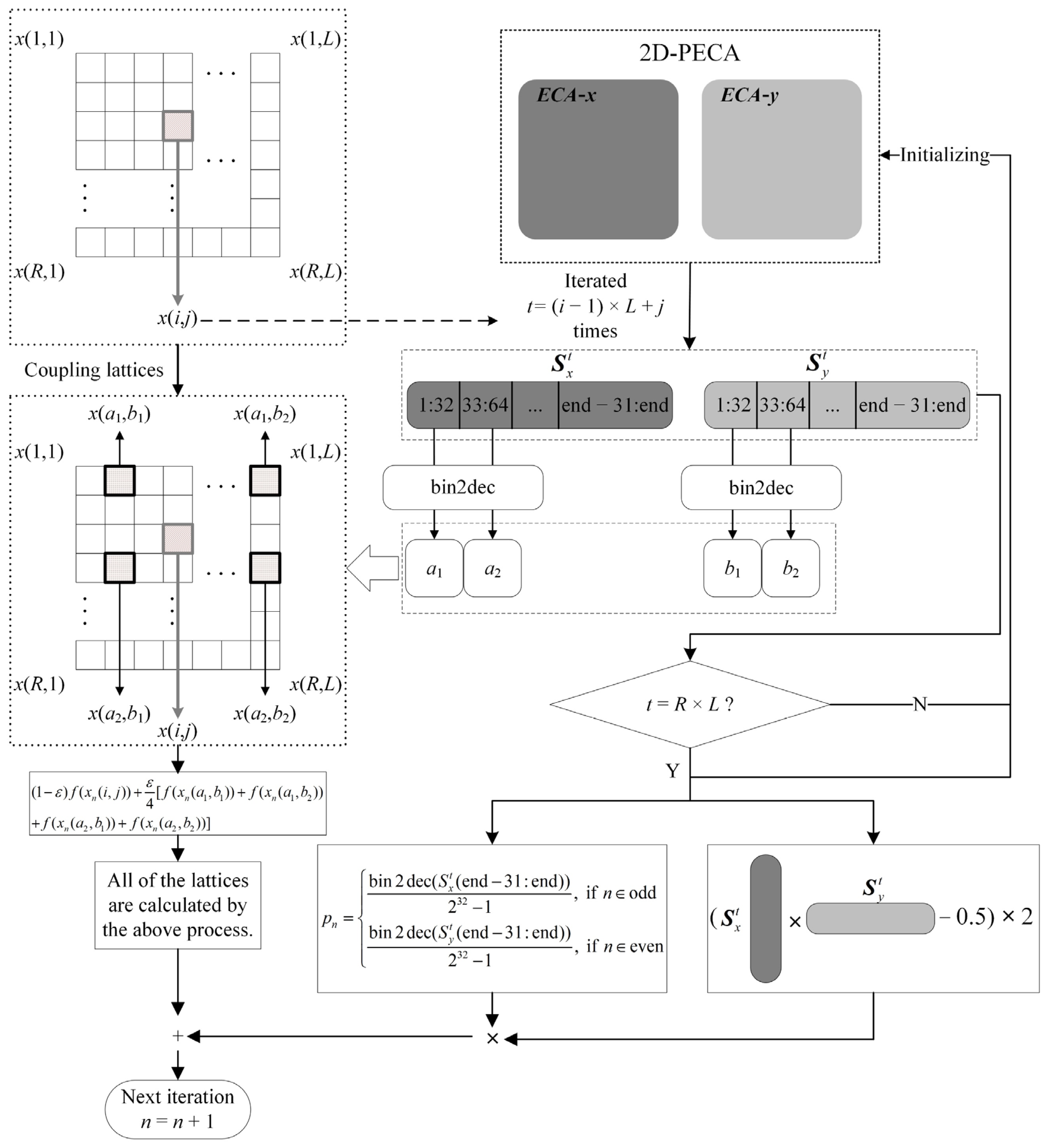
3. Introduction of 2D-DPRCML
The 2D-PECA is employed for dynamic pseudo-random coupling and perturbing the proposed 2D-DPRCML system. We assign two ECAs in 2D-PECA as
x and
y, respectively. A single ECA contains
M cells. The 2D-DPRCML system contains
lattices. The proposed system is described as follows:
In Equation (8),
i = 1, 2, 3, …,
R and
j = 1, 2, 3, …,
L denote the system’s row and column indexes, respectively. Both
n and
t stand for time series. In addition,
n =
n + 1 when all the lattices are iterated once.
t =
t + 1 when 2D-PECA is iterated once. From Equation (8), we can find that the updated value of each lattice is influenced by itself and the four coupling lattices during the iteration of the system. Such a process occurs in all lattices in each iteration. In other words, the coupling process enables the influence of each lattice to gradually spread to the other lattices as the system iterates, which can be regarded as the mutual perturbation between the individual lattices. This perturbation enables the system to have a more complex dynamical behavior. The relationship between
n and
t is shown in Equation (9), where the floor (
x) corresponds to the largest integer less than or equal to
x.
ε (
ε ∈ (0, 1)) stands for the coupling coefficient. A modulo operation is denoted by mod and returns the remainder of a division.
x mod 1 is associated with obtaining the decimal component of
x, and keeps the outcome of Equation (8) in the interval (0, 1). Moreover,
a1,
a2,
b1 and
b2 are pseudo-randomness coordinates of coupled lattices calculated in Equation (10), whereby
a and
b represent the row and column indexes, respectively.
and
are iterative results of
x and
y in the 2D-PECA separately at
t times.
ci is the
ith cell in an ECA, and its value is in {0,1}, thus the iterative result
c1c2c3…
cM can be expressed as a binary number as in Equations (10) and (12), or as a vector in GF(2) as in Equation (13). bin2dec(•) is the conversion from binary to decimal. In addition, the purpose of Equation (11) is to handle the conflict.
Equation (12) is the formula for calculating the perturbation
pn, in which the operation is determined by the time
n. The result of
pn is also in the interval (0, 1). There are two reasons for designing different expressions for the perturbation coefficient for even and odd clock cycles: the first is to improve data utilization. Since there are two dimensions of 2D-PECA, the different odd and even clock cycles allow the iterative results of both dimensions to be utilized. The second is to extend the perturbation period further. Although the ECA is long-periodic, its period is always limited by the number of cells to less than 2
M, so the added perturbation cannot exceed this period. If different perturbations are added by odd-even transformation, and the perturbations are obtained from different ECAs in the 2D-PECA, the perturbation period can be significantly extended, theoretically reaching a maximum period of 2
2M. The introduction of perturbation enhances the complexity and effectively alleviates the degradation in the chaotic system [
12]. It should be noted that the number of cells
M in
x or
y is larger than the largest of 64,
R and
L.
is a sign matrix calculated as Equation (13), in which
and
are row vectors in GF. (2), and its result is an
matrix containing the elements ‘−1’ and ‘1’. In Equation (13), we intercept the first
R and the first
L cells in ECA
x and ECA
y, respectively, to generate the sign matrix, ensuring that every lattice in the system can correspond to a sign in the sign matrix. In addition to reducing dynamical degradation, another purpose of adding perturbations is to reduce the correlation between different lattices [
12]. If we simply add the same perturbation to all lattices in each iteration without the sign matrix, the lattices will still be strongly correlated due to the coupling. The purpose of designing the sign matrix is to add perturbations with different and varying signs to each lattice during the iterations of the system, which successfully diminish the correlation between different lattices. The process of
nth iteration in the 2D-DPRCML system is portrayed in
Figure 2.
As shown in
Figure 2, the choice of coupled lattices is determined by the iterative results of 2D-PECA. 2D-PECA is iterated once to update the value of
a1,
a2,
b1 and
b2 before calculating the value of one lattice. Consequently, when 2D-PECA is in chaos,
a1,
a2,
b1 and
b2 are pseudo-random and dynamic rather than fixed as in Refs. [
29,
30].
4. Analysis on the Features of 2D-DPRCML
For comparison purposes, we separately set the control parameters to
μ ∈ (3, 4) and set the coupling coefficients to
ε ∈ (0, 1). The number of lattices
is
. In the 2D-DPRCML system,
x1(1,1) is set to 0.05, and the logistic map’s initial value is also set to 0.05. Then, we let the logistic map iterate 99 times to fill the rest lattices (
x1(1,2),
x1(1,3), …,
x1(10,10)). As for the 2D-PECA, the number of cells in both ECAs (
x and
y) is 100. Two random numbers of size 100 bits are utilized for initializing
x and
y, respectively, which are set as follows:
where
and
are represented as two hexadecimal numbers. As the rules for
x and
y, 102 and 105 are chosen, respectively, which ensures that the 2D-PECA is in chaos.
In the subsequent comparative analysis, we compare the proposed system with the conventional two-dimensional coupled map lattices (2D-CML) system based on adjacent coupling. In addition, we also compare the proposed system with the 2D nonlinear coupled map lattices (2D-NLCML) system [
29,
30] based on the chaotic Arnold cat map, and the 2D mixed pseudo-random coupling PWLCM-Sin map lattices (2D-MCPML) system [
7] based on pseudo-random coupling with a novel PWLCM-Sin map.
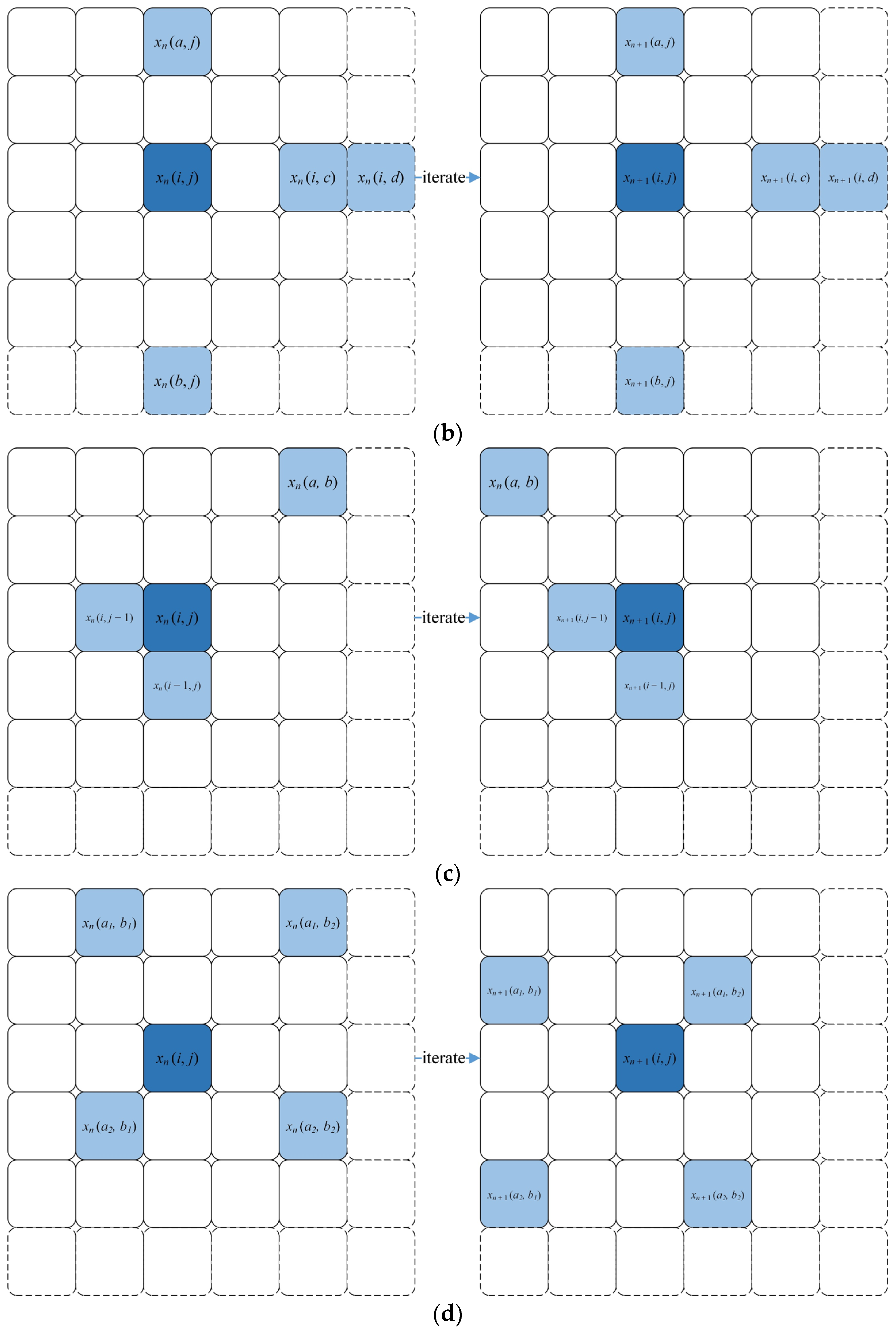
4.1. Analysis on Coupling Scheme
The conventional 2D-CML system’s coupling method is adjacent and fixed. The coupled lattices of
xn (
i,
j) in 2D-CML are always
xn (
I + 1,
j),
xn (
I − 1,
j),
xn (
i,
j + 1) and
xn (
i,
j − 1) at each iteration.
Figure 3a illustrates 2D-CML‘s coupling method.
The indexes of the coupling lattices for 2D-NLCML are calculated from the Arnold cat map:
in which
p and
q are control parameters. The number of the lattices is
. The coupled lattices are denoted by
xn (
a,
j),
xn (
b,
j),
xn (
i,
c) and
xn (
i,
d). Even though Equations (15) and (16) are nonlinear and some values of
p and
q can lead to chaos,
p and
q are fixed at each iteration. Moreover, Equations (15) and (16) only iterate one time in the system. Thus, the coupling lattices of
xn (
i,
j) are invariant in any iteration. It means that this system’s coupling method is non-adjacent and fixed, as shown in
Figure 3b.
The coupling method is improved in 2D-MCPML and is not fixed as in the above two systems. Besides the two adjoining lattices
and
, a non-adjacent lattice
with a random location is also coupled with a lattice of
. Furthermore,
a and
b are decided by the state value of
. For instance, we assign the size of the lattices as
if
,
and
. Therefore,
a and
b are changed at each iteration, increasing the instability of potential periodic orbits, and enhancing the system’s complexity. The coupling of a 2D-MCPML system is illustrated in
Figure 3c.
In contrast, the coupling method in 2D-DPRCML presented in
Figure 3d varies considerably from that of the above three systems. This coupling scheme is somewhat similar to Leon Chua’s method of selecting neighboring cells in cellular neural networks [
40]. However, in the proposed scheme, the coupling lattices are not centered on the current lattice, and only four lattices are involved in the coupling rather than all lattices in a range. Its coupling is pseudo-random and dynamic rather than fixed or adjacent. The four coupled lattices break the constraints of row
i and column
j, and they can be lattices at any position in the system. Moreover, the four coupled lattices are all changeable at each iteration. Thus, the complexity of the system is enhanced efficiently.
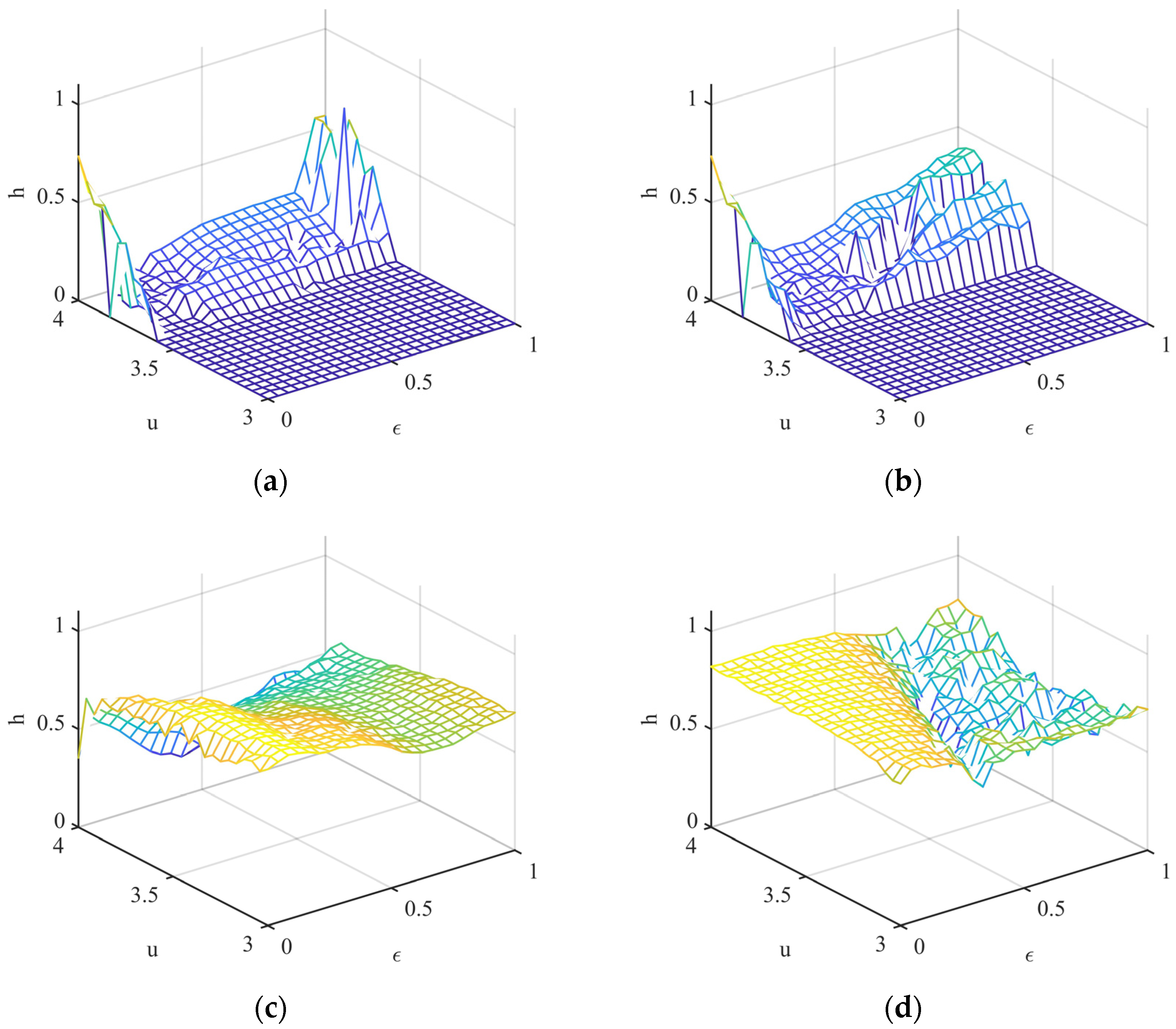
4.2. Analysis on the Lyapunov Exponent and Kolmogorov-Sinai Entropy
The Lyapunov exponent (LE) [
4] is a vital measure for evaluating the separation rate of infinitely approaching trajectories in phase space. It is a universal methodology for characterizing the predictability of dynamic systems. It is defined as:
where
λ stands for the LE of a dynamic system
and
i stands for the time dimension. The system requires at least one LE greater than zero to be in chaos. In addition, the higher the
λ, the better the system exhibits chaotic properties. Without loss of generality, we employ the Wolf method [
41] utilized in the literature [
6,
26,
27] to calculate LE. On this basis, Kolmogorov-Sinai entropy density (KED) is the mean value of LEs greater than zero in all lattices. It is introduced to characterize the chaotic properties of the system [
1,
4,
27]. The KED is calculated as follows:
in which
h denotes the KED and
λ+ is the positive LE of
lattices. Here,
i and
j are space dimensions. An
h value higher than zero means that the system contains lattices existing in chaos. Moreover, the magnitude of
h determines the strength of the system’s chaotic properties. The performance of the KEDs of the four systems is displayed in
Figure 4.
In
Figure 4, the X-axis, Y-axis and Z-axis denote coupling coefficient
ε, control parameter
μ and KED
h, respectively. In
Figure 4a,b, the KEDs of these two systems are positive only when
μ > 3.6, which means that chaotic lattices only exist in interval
μ ∈ (3.6, 4]. Moreover, the chaos is weak around
ε = 0.2 in the 2D-CML system shown in
Figure 4a, while this drawback is ameliorated in 2D-NLCML shown in
Figure 4b. In the first two systems, only 2.24% and 1.12% of the parameter pairs, respectively, make the system’s KED higher than 0.5. By contrast, as shown in
Figure 4c,d, 89.76% and 97.76% of the control parameters in 2D-MCPML and 2D-DPRCML, respectively, make the KED of the system higher than 0.5, and some KEDs of these two systems even reach 0.8. The KEDs of these two systems are positive in the entire interval of
ε and
μ. All the above analyses indicate that the chaotic behaviors of the latter two CMLs are stronger than those of the former two systems. Additionally, more parameters are available to be used as keys when the latter two systems are employed in cryptosystems. In other words, using 2D-MCPML and 2D-DPRCML systems can efficiently broaden the key space of cryptography. Furthermore, the minimum and average values of KED in
Figure 4d are 0.4266 and 0.7034, respectively, which are higher than 0.1994 and 0.6487 in
Figure 4c. Therefore, the chaotic properties of 2D-DPRCML are superior to those of 2D-MCPML.
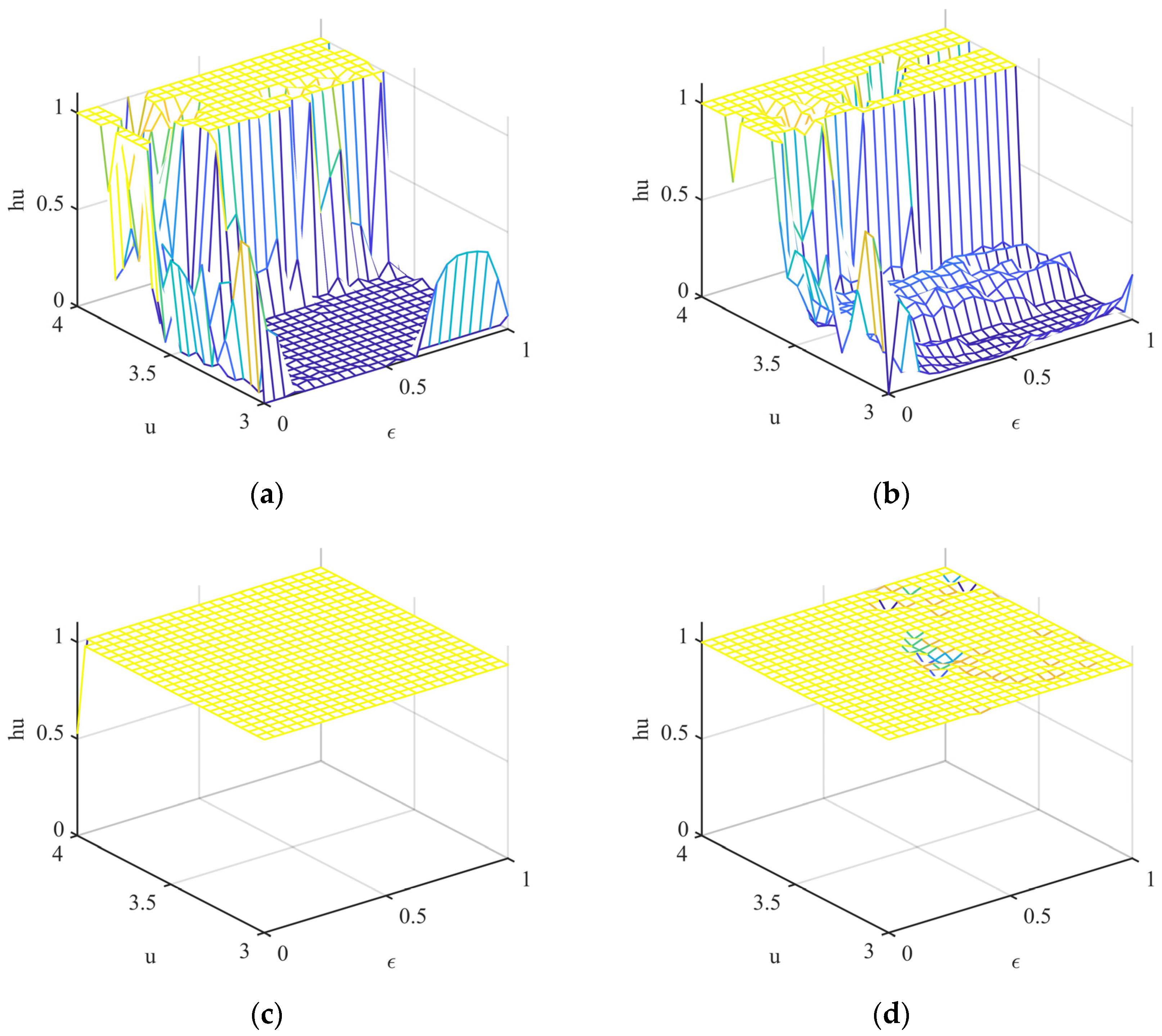
In addition to the KED, Zhang [
22,
42] proposed the Kolmogorov-Sinai entropy breadth (KEB) to indicate the proportion of chaotic lattices in the CML systems. The KEB is calculated as follows:
in which
hu is the KEB.
L+ refers to the number of lattices where LE is greater than zero. The system’s lattice count is indicated by
L. KEB which is employed to evaluate the chaotic performance of the spatiotemporal chaotic system from the spatial perspective. A larger
hu value implies that more lattices are in chaos, and the system possesses stronger chaotic properties. The KEBs of the four systems mentioned above are shown in
Figure 5.
In
Figure 5a,b, the KEBs reach ‘1’ only when
, which corresponds to the KEDs in
Figure 4a,b, which means that all lattices are in chaos only when
in 2D-CML and 2D-NLCML systems. Moreover, only 28.96% and 29.76% of KEBs reach ‘1’ in
Figure 5a,b, respectively, indicating that the chaotic properties of these two systems are weak. In contrast, the chaotic lattice exists under the entire interval of control parameters in 2D-MCPCML and 2D-DPRCML presented in
Figure 5c,d. Furthermore, 99.84% and 92.8% of KEBs reach ‘1’ in
Figure 5c,d, respectively. In addition, the minimum of KEBs reaches 0.95 in
Figure 5d, implying that at least 95% of lattices are chaotic in 2D-DPRCML, indicating the proposed system’s stronger chaotic properties.
4.3. Bifurcation Diagram
Bifurcation indicates period doublings, such as doubling from a single fixed point to two. In chaotic systems, this phenomenon may appear as the control parameters change. It is utilized to illustrate the period doubling in a chaotic system, and it can also be employed to assess the aperiodicity of a chaotic system.
In our research, we assign the coupling coefficient
ε = 0.375. The constant
σ = 0.5 in 2D-MCPML [
7]. Without loss of generality, the bifurcation diagrams of lattice
x (5, 5) in the systems mentioned above are depicted in
Figure 6.
From
Figure 6a,b, we can see that the periodic windows exist in these two systems, and it is apparent that 2D-CML outperforms 2D-NLCML in terms of aperiodicity when
. Moreover, the iterative results can fill the whole interval (0, 1) only for
in
Figure 6a,b. In comparison, as
Figure 6c,d illustrates, the periodic windows disappear in 2D-MCPML and 2D-DPRCML, and there is no fixed or periodic point in these two systems. Furthermore, as illustrated in
Figure 6d, the performance of 2D-DPRCML is the best in the four systems mentioned above since the outputs are able to fill the whole interval irrespective of the size of the control parameter
μ. In other words, the 2D-DPRCML system is chaotic throughout the control parameter interval (
μ ∈ [3,4]). Therefore, the aperiodicity is enhanced significantly in the 2D-DPRCML system. In addition, the space of optional parameters leading to chaos is expanded efficiently. Accordingly, the key space will be enlarged when the 2D-DPRCML system is employed for building a crypto-system.
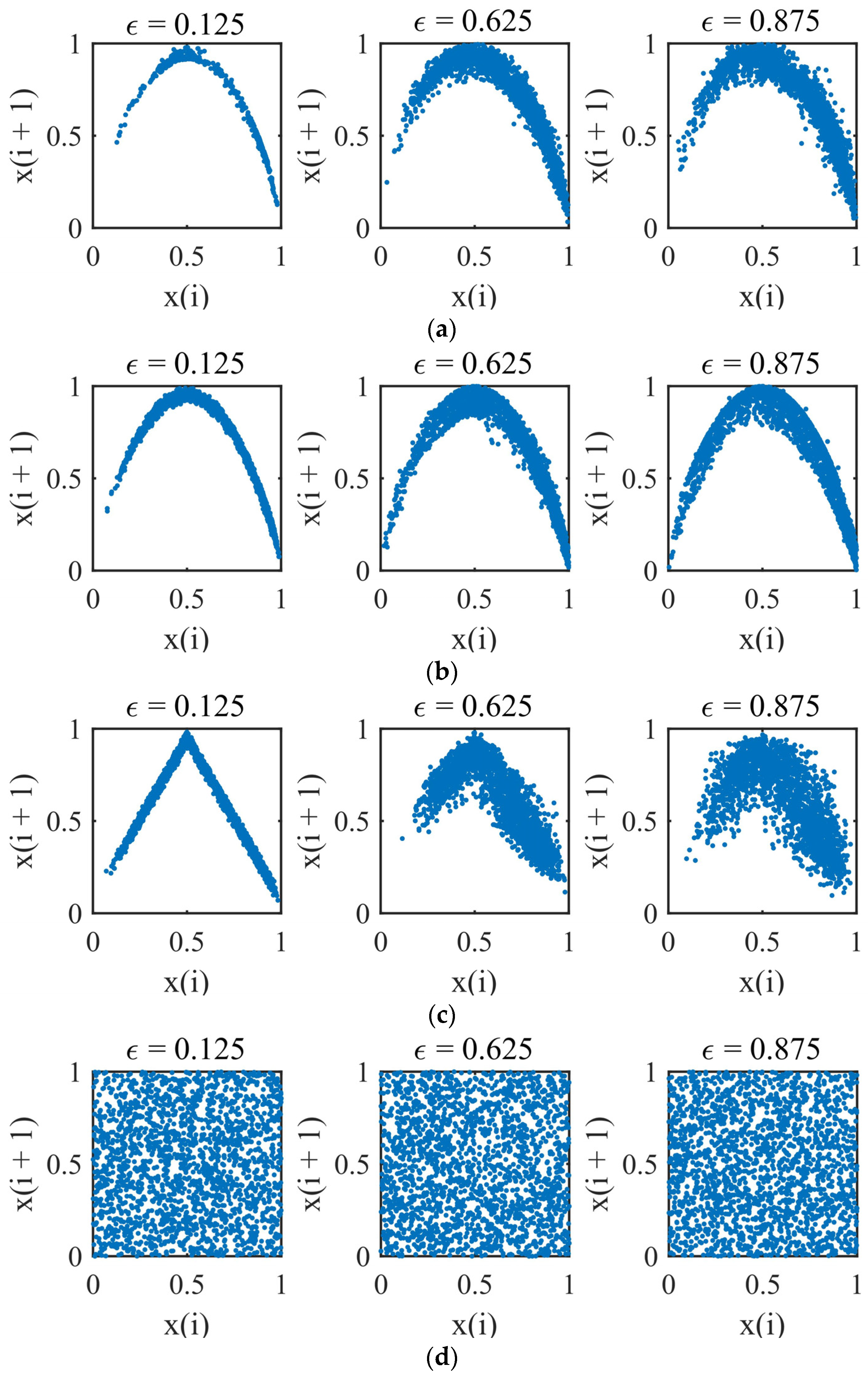
4.4. Return Map and Uniformity Analysis
The return maps can be employed to assess the uniformity of the sequence generated by a chaotic system. Furthermore, the character of a return map can be employed to judge whether the chaotic system is able to withstand attacks by the return maps approach [
32,
43].
We assign
μ to 4. The sequences selected for describing return maps are generated by lattice
x (5, 5) in these four systems. The return maps are listed in
Figure 7.
From the results displayed in
Figure 7a–c, the points in the maps progressively scatter as
ε increases. Nevertheless, the shape of the return map is clearly recognizable. Thus, an attacker can easily attack these three systems through the return map approach. Moreover, the return maps are prone to change with
ε in
Figure 7a–c. It implies that the change of coupling coefficient can influence the chaotic behaviors of 2D-CML, 2D-NLCML and 2D-MCPML systems. In contrast, the return map in 2D-DPRCML is insensitive to
ε because the points in
Figure 7d are uniformly distributed in phase space irrespective of the
ε. Hence, the space of the optional coupling coefficient in the proposed system has been enlarged. Furthermore, the unrecognizable shape of the return map means that the return maps method or phase-space reconstruction is ineffective for the 2D-DPRCML system.
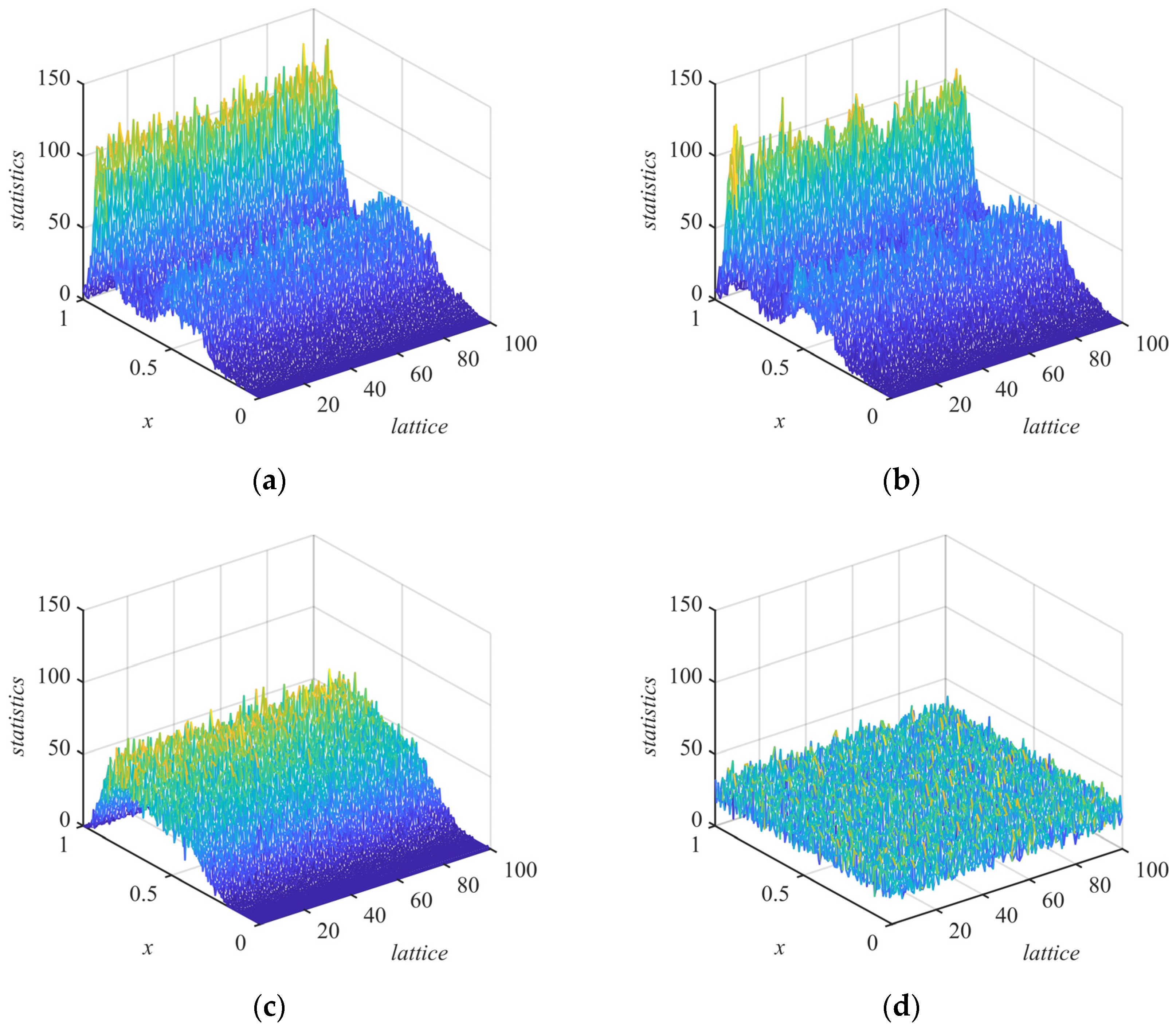
In addition to analyzing return maps in phase space, the uniformity of the chaotic system’s output sequence is another essential measure for evaluating the system’s randomness. In this paper, we set iteration number
, coupling coefficient
and control parameter
in chaotic systems. Then, the 100 sequences that are 5000 in length produced by the 100 lattices in the 4 chaotic systems mentioned above are acquired, respectively. The range from 0 to 1 is equally partitioned into 200 segments, and the points of the sequences acquired in every segment are measured. Statistical results are illustrated in
Figure 8.
In
Figure 8, the
X-axis denotes the segments in the range (0, 1), the
Y-axis denotes the indexes of the
lattices and the
Z-axis represents the number of points in a segment. It is clear that the points of sequences generated by the first two systems shown in
Figure 8a,b are primarily centered around the zones 0.8 and 0.5. Moreover, in
Figure 8c, the sequence points produced by 2D-MCPML are mostly distributed in the interval [0.5, 0.8]. On the contrary, the points in
Figure 8d uniformly distribute throughout the interval (0, 1), indicating that the sequences produced by any lattice in 2D-DPRCML possess better uniformity. Consequently, the uniformity of our system outperforms that of the system in
Figure 8a–c.
4.5. Correlation Analysis
In traditional spatiotemporal chaotic systems, coupled processes cause high correlations among lattices. At the same time, the literature [
44] points out that whether in temporal or spatial dimensions, the correlations of CMLs are sensitive to the coupling coefficient and control parameter. However, high correlations make it easy for an attacker to infer a particular lattice’s output from some given lattices’ outputs, causing the cryptosystem to be insecure when CML is applied to the cryptosystem. Therefore, analyzing the correlation of spatiotemporal chaotic systems is helpful in assessing their applicability to cryptosystems. In this paper, we let the system iterate 5000 times and obtain the output sequences of all lattices, after which we calculate the Pearson correlation coefficients between these sequences and derive the mean value. Similarly, the mean values of Pearson correlation coefficients are calculated for all pairs of parameters. We plotted these values to obtain the correlation analysis of the four systems under different parameter pairs, which are presented in
Figure 9.
In statistics, the correlation intensity between any two variables is judged by the Pearson correlation coefficient
ρ. The correlation intensities are weak and irrelevant when
ρ ∈ [0.2, 0.4) and
ρ ∈ [0, 0.2), respectively. In the two systems shown in
Figure 9a,b, when
μ ∈ [3.5, 4] the correlation coefficients rapidly as
μ increases, indicating that the correlation coefficients of these two systems are sensitive to the coupling coefficients. The overall correlation coefficients of 2D-CML are even lower than those of 2D-NLCML when
μ ∈ [3.5, 4] and
ε ∈ [0.5, 1]. In addition, the average of the correlation coefficients were below 0.4 for only 10.6% and 8.96% of the parameter pairs in the systems presented in
Figure 9a,b, respectively. At the same time, 79.48% and 76.84% of the cases in the first two systems result in correlation coefficients higher than 0.8, respectively. In addition, almost all correlation coefficients in these systems are equal to 1 when
μ ∈ [3, 3.5], indicating that the sequences produced by different lattices in the first two systems are closely related to each other that make them insecure when applied to cryptosystems. By contrast, 2D-MCPML and 2D-DPRCML optimize the correlation between the lattices significantly, but the correlation coefficient of the 2D-MCPML system increases rapidly as
μ approaches four. Furthermore, 92.72% and 98.08% of the parameter pairs in
Figure 9c,d, respectively, make the correlation coefficients less than 0.4, demonstrating that the correlation among any 2 sequences produced by various lattices is significantly decreased in the latter 2 systems. The low correlation coefficients of the 2D-DPCML make an attacker less likely to extrapolate a particular lattice’s output from known lattices’ outputs, demonstrating that it can enhance the security of cryptosystems when it is applied to them.
4.6. The NIST Test
The National Institute of Standards and Technology (NIST) SP800-22 suite, as an important test tool, is commonly used to assess the randomness of sequences, and it consists of 15 subtests [
45]. In these tests,
p-value refers to the degree of randomness of the tested sequence.
p = 1 denotes that the sequence is perfectly random, and
p = 0 denotes that the sequence is totally non-random. The significance level
α is typically a decimal number between 0.001 and 0.01. In this paper, we set
α = 0.01. If the
p-value is higher than 0.01, then the tested sequence is random, and the reliability of the test is 99%. Otherwise, the tested sequence is non-random.
In our test,
μ is set to 4, and
ε is set to 0.375. We let 2D-DPRCML iterate 50,000 times to obtain the test sequence, and then we eliminate the first 10,000 points in the sequence to minimize the influence of starting values. We selected the sequence
produced by the lattice
x(6, 5) for testing, and the decimals in the sequence are quantized to 32bit unsigned numbers as follows:
in which the length of
is 10
6 bits, which is used for testing.
Table 3 displays the testing results.
It can be seen from
Table 3 that the 2D-DPRCML’s output sequence passes all the subtests. In addition, we also test the sequences generated by the lattices
x(1, 3),
x(5, 4) and
x(10, 7), and all of them pass the randomness test. For comparison purposes, we performed a pass frequency-based test [
45] on the sequences produced by the four systems, and the results are presented in
Table 4.
In
Table 4, it is clear that the first three systems’ output sequences rarely pass the frequency test, which is the reason why the sequences generated by these chaotic systems cannot be directly used in cryptosystems [
12,
46]. In general, when chaotic systems are applied to cryptosystems, bit-extraction algorithms and nonlinear functions are commonly used to obtain better randomness and uniformity. However, the proposed 2D-DPRCML system exhibits excellent chaotic properties even without using the above methods, which is a good indication of its promising applications in cryptography.
5. Conclusions
By employing 2D-PECA for building a 2D spatiotemporal chaotic system, this paper proposes a novel 2D-DPRCML system. There are three innovations in the proposed system: a dynamically pseudo-random coupling scheme based on the iterative results of 2D-PECA, the introduction of perturbations generated by the 2D-PECA and the different and variable sign of perturbation for each lattice. The simulation and comparison analysis results demonstrate that the 2D-DPRCML system possesses stronger chaotic properties, including higher KED and KEB, and better aperiodicity in the bifurcation diagram. The good chaotic behavior of 2D-DPRCML enlarges the optional parameter pair space, which indicates that the key space can be extended when the proposed system is implemented in cryptography. Moreover, the return map in phase space is uniform, implying that 2D-DPRCML is resistant to the attack of phase-space reconstruction. Statistics and simulation results illustrate the excellent uniformity, randomness and unpredictability of 2D-DPRCML’s output sequence. Additionally, the correlation intensity among any two lattices in this system is weak, thus strengthening the system’s security. To sum up, all these good properties of 2D-DPRCML enable it to be well applied in the field of cryptography, such as the S-box generation, pseudo-random number generators and image encryption.


