Exploiting Stacked Autoencoders for Improved Sentiment Analysis

Abstract

Sentiment analysis is an ongoing research field within the discipline of data mining. The majority of academics employ deep learning models for sentiment analysis due to their ability to self-learn and process vast amounts of data. However, the performance of deep learning models depends on the values of the hyperparameters. Determining suitable values for hyperparameters is a cumbersome task. The goal of this study is to increase the accuracy of stacked autoencoders for sentiment analysis using a heuristic optimization approach. In this study, we propose a hybrid model GA(SAE)-SVM using a genetic algorithm (GA), stacked autoencoder (SAE), and support vector machine (SVM) for fine-grained sentiment analysis. Features are extracted using continuous bag-of-words (CBOW), and then input into the SAE. In the proposed GA(SAE)-SVM, the hyperparameters of the SAE algorithm are optimized using GA. The features extracted by SAE are input into the SVM for final classification. A comparison is performed with a random search and grid search for parameter optimization. GA optimization is faster than grid search, and selects more optimal values than random search, resulting in improved accuracy. We evaluate the performance of the proposed model on eight benchmark datasets. The proposed model outperformed when compared to the baseline and state-of-the-art techniques.

1. Introduction

Numerous sources of unstructured data are being produced every day as a direct result of the proliferation of social media. The analysis of these data for polarity detection is rather difficult. Opinion analysis and opinion mining are other terms for sentiment analysis. Emotion detection is a fundamental aspect of natural language processing (NLP), since it involves determining the feelings conveyed by text. Feelings might be good, negative, apathetic, or indifferent. Sentiment analysis primarily focuses on urgency, emotion, polarity, intention, and feelings. The sentiment analysis can be categorized to deal with a particular issue depending on the desired outcome. Sentiment analysis comes in many forms, including aspect-based, fine-grained, emotion detection, and multilingual sentiment analysis (MLSA).

Sentiment analysis, whether at the sentence, sub-phrase, or document level, is performed using machine learning techniques with varying degrees of success depending on the goal. Sentence-level sentiment analysis determines the emotions present in a sentence. Sub-sentence sentiment analysis is a complex form of sentiment analysis (SA) that determines the sub-expressions present in a sentence. With document-level sentiment analysis, you can obtain an overall impression of the tone of a piece of writing.

Both supervised and unsupervised machine learning algorithms can be employed for SA. The difference between these types is that the supervised algorithm needs a labeled dataset. An unsupervised machine learning algorithm, on the other hand, can analyze a dataset that has not been labeled. A supervised machine learning algorithm will produce results based on previous learning. It is extensively used for deciphering real-world computing problems. It is not possible to construct a large, labeled dataset for classifying text. Therefore, unsupervised machine learning (ML) is the best choice for textual data analysis. These algorithms can determine the hidden structures and associations in data. Combining two or more ML models and deep learning (DL) for the purpose of sentiment analysis can lead to great improvement in performance. DL algorithms are advanced machine learning techniques, as they are inspired by the human brain. DL algorithms can process a large volume of data with little human effort. In the case of ML, human input is necessary to rectify possible mistakes, while on the other hand, a deep learning algorithm can correct itself by learning through algorithm chains. The training stage of a deep learning algorithm takes a more prolonged length of time, but once it is trained it can solve intricate problems. Various studies have used DL models for the task of SA. For example, commodity market SA [1], financial SA [2], aspect-based financial SA [3], investor sentiment analysis [4], biomedical SA [5], clinical analytics SA [6], and social media SA [7,8,9]. Both deep neural networks and shallow neural networks can assess any task. However, an exclusive advantage of the deep neural network over the shallow neural network is that it can perform feature extraction along with learning tasks. This is due to intermediate hidden layers [10,11] being used to extract better features. In contrast to deep neural networks (DNNs), which typically have multiple hidden layers of varying sorts, shallow NNs have only one hidden layer. DL algorithms can achieve an identical level of accuracy more efficiently in terms of a number of parameters and computations. DNNs learn a new and abstract representation of the input, at every layer, for creating deep representations. Every single deep learning model has its pros and cons, and can be efficiently applied in a single domain. A hybrid strategy, a means of merging two or more models, was proposed by [12,13] for obtaining the benefits of both models and overcoming their flaws. Within the realm of opinion mining, in [13], researchers integrated a semantic knowledge base with machine learning, which resulted in a 5% increase in accuracy. Another study [12], obtained a 4% improvement in accuracy by combining lexicon with machine learning. Therefore, it is obvious that combining two or more models can address challenges that exist in a single model and help in improving performance. However, the efficiency of hybrid models may vary depending on the task.

In addition, there are a variety of social network data inputs, such as tweets and reviews. Both the sizes of tweets and reviews, as well as topic diversity and sample size are different in each of these datasets. The presence or absence of clear sentiments or unnecessary information is likewise different between datasets. There is a chance that some approaches fall short in terms of sentiment accuracy and performance [14,15]. Various data types are inapplicable to specific techniques. Our research raises the question of whether optimized hybrid models outperform single models independent of the dataset peculiarities. As a result, we test an optimized hybrid model on datasets from different domains.

In this paper, we investigate a deep learning model for sentiment analysis. Our investigation was guided by the following research questions (RQs):

• (RQ1) Does the genetic algorithm (GA) perform better than grid search and random search for hyperparameter optimization of stacked autoencoders (SAEs)?
• (RQ2) Can the hybrid model perform better than the individual model with optimized hyperparameters?

To address the above research questions, we focused on analyzing tweets and reviews to detect polarity sentiments in eight benchmark datasets. Specifically, we developed a deep learning framework that is effective at detecting the actual sentiment behind social media tweets (short text) and reviews (long text).

The major contributions of this paper are as follows:

• A hybrid model GA(SAE)-SVM is proposed which produces better results than other familiar deep learning models.
• To reduce the computational cost and increase the accuracy, GA is used for hyperparameter optimization of SAE.
• Eight standard datasets for sentiment analysis are used to assess the performance of the proposed model.

The remainder of the study is structured as follows: Section 2 provides a literature review. In Section 3, the research foundations are outlined. The methods proposed are described in Section 4. The experimental results are provided in Section 4. Section 5 contains the conclusion and recommendations for future work.

2. Literature Review

The research goals center on developing a more precise hybrid model for sentiment analysis. This section discusses prior work in the field of sentiment analysis, including the most recent research in the field of SA and optimization with GA.

2.1. Sentiment Analysis

The basic classification or clustering module of most classic sentiment analysis research papers relied on supervised machine learning approaches [16]. When displaying and classifying user-provided texts for emotional intent, these systems frequently used the BOW model and n-gram features [17]. N-grams are continuous sequences of words, symbols, or tokens in a document. The simple bag-of-words (BOW) model has a number of drawbacks, including the inability to account for word order and syntax [17]. In particular, the high-dimensional feature space generated by utilizing n-gram features is a major problem [18]. Many recent research studies [19,20] have made substantial use of feature selection approaches to try to solve this issue.

Linear discriminant analysis (LDA), support vector machine (SVM), naïve Bayes (NB), and artificial neural networks (ANNs) are the most prevalent and most effective classification algorithms for detecting sentiment from user-generated text [21,22,23]. Some of the most common drawbacks of using these supervised algorithms are that they require a huge quantity of training data and are sometimes very slow. Unsupervised lexicon-based approaches have been proposed [17,24] to overcome these issues. These approaches are straightforward, quick, and adaptable. However, because they rely so much on the lexicon approach, they are less accurate [24,25] than those that are closely overseen. Furthermore, lexicon-based approaches are limited in their applicability to domains without a well-defined vocabulary because of their domain dependency.

Few researchers have attempted to combine supervised and lexicon-based methods to benefit from them [26,27]. For tweet sentiment analysis at entity level, [28] merged supervised and lexicon-based techniques. High precision and recall were obtained from lexicon and supervised methods, respectively. An approach for concept-based sentiment analysis that incorporates both lexical and machine learning methods has also been developed [29]. The created solution was superior to both purely lexicon-based methods and purely statistical methods for identifying polarity and sentiment strength, and it also provided a more convincing explanation and justification. A novel hybrid approach to sentiment classification was recently devised [30], with the promise of locating and paring down an acceptable Twitter-specific vocabulary collection. Last but not least, in [31], a hybrid machine learning/lexicon-based approach to sentiment polarity is presented. These authors compared the hybrid approach to statistical and lexicon-based classifications of user reviews, and found that the latter were superior, while the former were more accurate.

Few studies have attempted to use hybrid DL models for sentiment analysis. In [32], a model for SA that is a fusion of long short-term memory (LSTM) and SVM is proposed. The IMDB movie review dataset was used for evaluation purposes. In [33], researchers created a hybrid heterogeneous support vector machine (H-SVM), specifically for SA, that combines features of both traditional SVMs and H-SVMs. Tweets related to COVID-19 were used to test proposed technique. In [34], researchers attempted to develop a generalized paradigm for sentiment analysis. In this research, the authors incorporated a convolutional neural network (CNN) into their algorithm for generating vectors from the review dataset. The dataset used for this study consisted of IMDB reviews (publicly available) and amazon reviews (collected by the authors). In [35], a hybrid model of CNN and SVM is proposed. fastText was used for embedding of Arabic text, CNN was used for feature selection and SVM was used as the final classifier.

Researchers have suggested a hybrid model to deal with the problem of classifying the ambience of both users and content [36]. Social context features are embedded in the model. Various datasets were used for the evaluation of the model. In the study by [37], the authors proposed a method to enhance the movie recommender system by incorporating sentiment analysis of reviews. The proposed method combined collaborative filtering and content-based methodology for improving the initial recommendation list. Initially, the concept of collaborative filtering was presented by [38]. Combining that method with sentiment analysis was used in [37]. The studies discussed above employed conventional methods of sentiment analysis.

Some of the recent research used other metaheuristic optimization methods for the task of sentiment analysis. In [39], researchers introduced a new method of the social spider optimization algorithm for sentiment categorization within a tagged Twitter dataset (SSA). This study demonstrated that social networks may be studied using optimization search techniques. When compared to other machine learning methods, their approach was found to be the most effective across a range of measures. In their study, [38] used the whale optimization algorithm (WOA) and social impact theory-based optimization (SITO) to analyze the sentiment analysis problem as an optimization and multiobjective problem. In addition, [40] combined sunflower optimization with chaos theory to provide a novel method for sentiment analysis. TripAdvisor data were used in their testing of the proposed approach.

2.2. GA Optimizer

One variety of metaheuristic algorithm is known as the GA. The idea of evolution is the primary source of inspiration for this technique, which is applied to search and optimization issues [41,42]. It works by imitating gene operations such as selection, crossover, and mutation. It is currently widely used in various fields [41,42,43,44,45,46,47,48]. A typical GA recommends a set of optimal solutions, and a fitness function is built to determine the effectiveness of each solution.

In previous studies, GAs were used for weight optimization [46,47], and to structure ANNs [44,45]. A study by [48] used GA for optimizing the CNN architecture of the CIFAR-10 image dataset. Findings showed that GA-generated CNN structures show good performance. When it comes to the automatic optimization of CNN architectures for visual classification on CIFAR-10, another study [49] used the Cartesian genetic programming encoding approach. In [50], GA was used to optimize hyperparameters. The fitness function was assembled by combining verification time and validation accuracy. Two datasets, motor fault diagnosis and MNIST, were used for assessment, and the results exhibited improvement in accuracy and efficiency. A study by [51] employed GA to tune the hyperparameters of a three-layer CNN.. Their findings revealed that hyperparameter searching can be optimized in less time with distributed GAs.

A few other studies used GAs for optimization. In [52], the authors used GA to obtain the optimal word vector to input into a hybrid model (CNN-BiLSTM) for the classification of online judgment. Another study, by [53], used GA for hyperparameter optimization of a CNN for the classification of handwritten numbers. In their research, [54] used a variable-length GA for CNN optimization and compared the optimization methods, including large-scale evolution, random search, and classical GA. The authors concluded that performance can be improved by expending more time on hyperparameter optimization. In [55], optimization methods including grid search, random search, and GA are compared. These algorithms were utilized for hyperparameter optimization of CNN for the image CIFAR-10 dataset. The authors concluded that random search is faster but does not guarantee good results. When the search space is large and there are too many parameters to be tuned, GA is the best option over grid search.

2.3. Current Status and Limitations

Through an extensive literature review, we reveal the persistence of sentiment analysis problems and the necessity for globally accepted automated sentiment analysis approaches. Few studies combined two or more deep learning models [32,33,34]. Most deep learning models were used for domain-specific datasets, so their validity cannot be generalized. In the current categories of methods, deep learning models are most effective for sentiment analysis. Determining the optimal values of a deep learning algorithm has a major effect on its performance. Various studies have used GA optimization [48,49,50] for different tasks. Using GA-optimized SAE for sentiment analysis is an intriguing and influential research concept.

3. Foundations

This section discusses the key ideas utilized in this research, such as SAE and GA.

3.1. Stacked Autoencoders (SAEs)

An autoencoder is an unsupervised neural network that is used to recreate a vector from its latent feature space, i.e., similar embeddings are kept closer to each other in a latent space. Autoencoding is an unsupervised neural network technique. The process of autoencoding proceeds as follows: initially, a vector is used as the input $p^{\left(k\right)}\in {\left[0, 1\right]}^m$, referring to the latent space as $d^{\left(k\right)}\in {\left[0, 1\right]}^m$. The encoding functionality, parameterized by $\theta =\left\{W, b\right\}$, is represented as

$$d^{\left(k\right)}=f\theta \left(p^{\left(k\right)}\right)=s\left(W{p}^{\left(k\right)}+b\right),$$

(1)

where $s$ is a nonlinear activation function such as a sigmoid function or hyperbolic tangent, $b$ is a bias vector, and $W$ is a $m\times m$ weight matrix. The latent representation $d^{\left(k\right)}\in {\left[0, 1\right]}^m$ is then mapped back onto a “reconstructed” vector, ${\widehat{p}}^{\left(k\right)}\in {\left[0, 1\right]}^m$, in input space

$${\widehat{p}}^{\left(k\right)}=g\theta \left(t^{\left(k\right)}\right)=s\left(W{t}^{\left(k\right)}+b\right),$$

(2)

The weight matrix W of the reverse mapping may optionally be constrained by $W=WT$, in which case the autoencoder is said to have tied weights [56,57]. The primary goal of training is to learn the parameters $\theta =\left\{W, b\right\}$, and ${\vartheta }^{\prime }=\left\{W, b\right\}$ is to reduce the average reconstruction error over a set of input vectors, i.e., $p^{\left(1\right)},\dots .,p^{\left(n\right)}$

$$\begin{gathered} \left(\theta .{\vartheta }^{\prime }\right) \\ \left(\theta .{\vartheta }^{\prime }\right)=\arg m\underset{\theta .{\vartheta }^{\prime }}{\underbrace{max}}\frac{1}{n}{\displaystyle \sum }_{k=1}^n Ls\left(p^{\left(k\right)}. {p^{\prime }}^{\left(k\right)}\right), \end{gathered}$$

(3)

$$\left(\theta .{\vartheta }^{\prime }\right)=\arg \underset{\theta .{\vartheta }^{\prime }}{\underbrace{min}}\frac{1}{n}{\displaystyle \sum }_{k=0}^{n}Ls (p^{\left(k\right)}. g\vartheta \prime \left(f_{\theta }\left(p^{\left(k\right)}\right)\right))$$

(4)

where $Ls$ is the loss function such that cross-entropy parameters $\theta$ and ${\vartheta }^{\prime }$ can be optimized by stochastic or mini-batch gradient descent.

Various autoencoders can be combined to form a DNN [56,57]. The combination of autoencoders can work as a centipede. The autoencoders will process the input vector in a nested manner, such that the output of the first autoencoders will be the input of the next one. Each level of autoencoders processes the related information from the latent space. Therefore, the resultant output has a multilevel representation of the input vector. This technique is very useful in feeding information into a classifier [58] or initializing a supervised neural network [59,60]. A graphical representation of the SAE is presented in Figure 1.

3.2. Genetic Algorithms (GAs)

The GA is an evolution-inspired metaheuristic search algorithm. Survival of the fittest among the population is used to ensure the species’ continued existence. Figure 2 below illustrates the GA flow.

The selection operator chooses the best chromosomes based on the evaluation or fitness function. The selected chromosomes will be used for reproduction [61,62]. Various selection methods have been proposed; fitness proportionate selection and linear ranking are the most prevalent [63].

Fitness proportionate selection, or roulette wheel [64] selection, selects the parents according to their fitness, i.e., the better the fitness, the higher the chance to be selected. It is very useful to avoid rapid convergence. In linear ranking, each individual is explicitly ranked according to their fitness. The selection of individual chromosomes depends on their fitness rank.

Crossover or recombination is used to generate offspring from the parents’ genetic information. This is applied to speed up the optimization process. Crossover frequency depends on the optimization problem, generally, and it is adapted to high probability values [65]. Various techniques are known, including single-point crossover, two-point crossover, and uniform crossover. Mutation is responsible for the exploration of chromosomes. In this process, a part of the chromosome information is changed to produce a new offspring. This is very useful to maintain genetic variability from one generation to the next [66].

This method is adapted to a very low probability value [65]. The selection, crossover, and mutation cycle will continue until they meet the optimization criterion or the stopping criterion. The stopping criterion can be a number of iterations. The selection of population size, crossover frequency, mutation probability, and fitness function affect the performance of GAs [63,67].

3.3. Support Vector Machines (SVMs)

The support vector machine (SVM) is one of the most popular supervised machine learning models. Its popularity is justified by its flexibility, usage, and applications. It is reported to be used for classification, regression, and outlier detection problems. It is very effective for both single- and multidimensional space. Its applications in the field of text classification have resulted in very high accuracy [68,69].

SVM is based on a linear learning pattern. It identifies an optimal decision boundary, known as a hyperplane. It exhibits a clear margin of split between classes for the extreme boundary points. Based on a supervised learning model, SVM tries to maximize space between the training points of each class to improve the classification performance [70]. The closest points to the hyperplane and the opponent class are known as support vectors. The optimal solution is always based on the support vectorsIn case a data point is not separable in a linear manner, the data point is transformed into a high-dimensional space using a kernel function. This will help to form a linear hyperplane in a higher dimensional space [71]. A kernel function reduces the computational cost of transformation, as it uses a dot product between two vectors so that each vector is represented in higher transformation space [72]. Various types of kernels are popular, including the polynomial kernel, RBF kernel, and sigmoid kernel. Multiple kernels can be combined to form a custom kernel. Choosing the best kernel is a frivolous task as it all depends on the classification problem.

4. Methodology

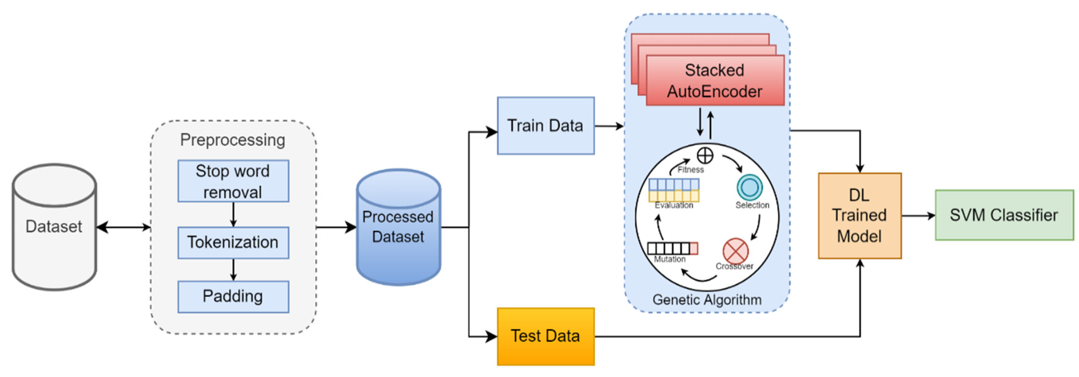
In this paper, we propose a GA(SAE)-SVM hybrid model for sentiment analysis. The SAE’s hyperparameters are optimized using the GA. The last classifier is the SVM. Figure 3 depicts the block diagram of the suggested model.

As shown in the diagram, after preprocessing, the dataset is divided into training and test sets. Each training dataset is used as an input into SAE. The GA determines the optimum value of the hyperparameters of the SAE for each dataset. In the hyperparameter optimization phase, selection, crossover, and mutation operations of the GA run for the selected number of iterations. Optimum values of hyperparameters are determined for each dataset by running these steps for several iterations. SVM is selected as a classifier. The purpose of choosing the SVM is due to its proven efficiency in NLP tasks [68]. It can be used for both classification and regression. For our research, we have used a linear SVM. Extracted feature vectors from GA-SAE are fed into the SVM for final classification. The steps described in the methodology are discussed in detail below.

4.1. Preprocessing and Building the Feature Vector

SA can be performed at different levels, including aspect/feature, sentence, or document level. Sentiment analysis based on documents is used in our study. For this purpose, we have used eight benchmark datasets. Training data need to be cleaned before being used as an input into the classification model. To achieve this, we engaged in the process of “cleaning” the text by eradicating unnecessary elements such stop words, punctuation, white space, special symbols, and URLs. After cleaning the text, a feature vector is built. Two methods are currently widely used for this purpose, i.e., TF-IDF and word embedding.

For this research, we use word embedding because of its proven supremacy over TF-IDF [14]. We use the Word2Vec model of word embedding for building feature vectors. Tomas Mikolov published Word2Vec in 2013 at Google [73]. It includes the continuous bag-of-words (CBOW) and skip-gram models. In this research, we use the continuous bag-of-words (CBOW) method. One disadvantage of using Word2Vec is that it does not support words out of its vocabulary. We dealt with this by creating a new token, [UNK], to use in place of terms that were not included in the dictionary. To eliminate the need for a unique token, we retrain Word2Vec on our lexicon dataset that contains terms that appear more than seven times. For deep learning models, a consistent input vector is essential. We pick l, a constant length, to use across all datasets. For reviews shorter than the defined length, a zero is added to the end of the vector. For reviews longer than the fixed length l, the back is instead abbreviated. However, information may be lost during the truncation process. To minimize this loss, fixed length should be chosen to minimize truncation. Our datasets are composed of tweets and reviews, therefore, we made sure the feature vector was as long as possible without going above the limit, so we would not lose too many samples. This technique is often used in the literature [74,75,76]. The following are the values chosen for the fixed length in this study: As tweets consist of a maximum of 280 characters, 280 is chosen as the fixed length for tweets. For review datasets, the fixed length is between 300 and 500 for each dataset, depending on the length of the samples. If the same fixed length is chosen for tweets and reviews, it may lead to loss of information or waste of memory.

4.2. Proposed SAE Architecture Using GA for Feature Extraction

This research proposes SAE for extraction features for classification. Hyperparameters such as momentum, batch size, hidden neurons, and epoch have a significant impact on SAE performance. Tuning the hyperparameters results in higher performance. The GA is employed to optimize the hyperparameters of SAE. The GA was inspired by the theory of evolution, and it works on the selection principles of nature. Applying the GA will result in finding the fittest values of hyperparameters to optimize SAE. The steps involved in the proposed solution, along with Algorithm 1, are presented below.

4.2.1. Initialization Phase

A vector input containing constituent values of SAE, including initialization mode, epoch, and learning rate, along with parameters for GA, including size of population and iterations, is supplied to the SAE. The number of solutions can be represented as $X_{N\times N_P}$, where $N$ is the population size and $N_P$ is the total number of optimization parameters. After SAE initialization, crossover and mutation are initiated for the GA parameters. In the GA, the population generation step is performed just once, but the subsequent steps are carried out repeatedly until the stopping requirement is met. There are two methods for population generation, i.e., random initialization and heuristic initialization. Random initialization for completely random solutions has been used in the proposed research. A randomly generated population can be represented as

$$x_{ab}=l_b+random\ast \left(u_b-l_b\right),$$

(5)

where $x_{ab}$ is a solution, $b$ is a parameter, $b$ is (1, $N_P$), $l$ is (1 to $N$), $u_b$ is the upper bound, and $l_b$ is the lower bound.

4.2.2. Evaluation Phase

The parameter is chosen during the initial phase of developing an SAE model. The SAE model is built using the training dataset. Previously, the dataset in question was separated into training and testing halves.

4.2.3. Update Phase

The current step involves picking a solution with a high fitness value, $x_b$. With the help of the GA’s operational flow, we update each solution in the solution space. The update process includes selection, mutation, and crossover operators. The evaluation and update phases are processed in a recursive cycle until the stop criterion is achieved.

Algorithm 1: Pseudocode of GA for SAE

Input: dataset,          /preprocessed data for classification/ pop_size X,                /size of population/ max_gen,          /to terminate the while condition/ C_prob,                /crossover probability/ m_prob                /mutation probability/ Output: optimized features X_train, x_test, y_train, y_test←train_test_split(Data) m ← 1 Generate initial population $X^m \leftarrow \{x_1^m,x_2^m,\dots ,x_{\mathit{pop}-\mathit{size}}^m\}$ Calculate F-Score $\left(x_i^m\right)$ for i=1,2,…, pop-size While m ≤ max_gen do  m ← m+1  k ← 1 while k ≤ pop_size do Select two chromosomes $x_a,x_b$ from $x^{m-1}$ Produce two chromosomes $x_a^{new},x_b^{new}from{x}_a\mathrm{and}{x}_b$ from c_prob Do mutation on $x_a^{new}\mathrm{and}{x}_b^{new}$ with m_prob Calculate F-Score $\left(x_a^{new}\right)$ and F-Score $\left(x_b^{new}\right)$ Add $x_a^{new}\mathrm{and}{x}_b^{new}\mathrm{into}{X}^N$  k ← k+1 end pick pop_size best chromosome from $X^{m-1}$ to from $X^m$   $x^{\mathit{best}}$  ← the best chromosome in $X^m$ End

An initial selRoulette selection is made between chromosomes $x_a$ and $x_b$. Using ordered crossover with a probability of cprob, we generate two novel chromosomes, $x_a^{new}$ and $x_b^{new}$. We then choose an ordered crossover that involves swapping genes between two parents to produce a new offspring. Mutation is performed by calling the mutShuffleIndexes operator, which is utilized to generate novel chromosomes with randomized fitness values. These are then incorporated into the new population, and the best chromosome, $x^{best}$, is chosen for selection. This loop persists until the termination condition holds. The F-score, together with the related hyperparameter values, is returned by the fitness function once the optimization process has finished. These optimal values are then used to train and evaluate the SAE model.

4.3. Hyperparameter Tuning

The feature vector built in the previous step is used as an input into the SAE. The values of the hyperparameters training epoch, L2 regularization, learning rate, and batch size of SAE are determined by GA. L2 regularization, also called ridge regression, adds the “squared magnitude” of the coefficient as the penalty term to the loss function. Momentum is used to reduce any oscillation that occurs due to noise. The range for momentum is 0.9–1. The range for learning rate is between 0.001 and 0.1. Learning cannot take place when the weight value is equal to 0. To address this issue and keep up with the learning procedure, a bias is applied to the total weight value [77,78]. To decrease the memorization of the model, L2 regularization is used in the training phase for better results. It prevents the overfitting of the model and reduces complexity without affecting performance. The range of values of L2 regularization is between 0.003 and 0.1.

For the GA, the number of parameter generation is set to 5, and population, crossover, and mutation were set to 10, 0.8, and 0.2, respectively. Four autoencoders are stacked together with 4, 8, 10, and 20 hidden neurons, respectively. In any deep learning base model, the activation function plays an important part in the activation and non-activation of neurons. The GA determines the activation functions ReLU and Sigmoid for the encoder and decoder, respectively, based on their performance. In the decoder, Sigmoid forces the output to the range [0, 1], hence improving the performance. For optimization, two optimizers were considered, Adam and Adadelta. GA determines the Adam optimizer for the encoding phase based on its performance. The loss function is used to standardize the autoencoder’s scores and generate a probability for each class. The loss function of cross-entropy is applied. During the encoding process, we made use of the Adam optimizer and a cross-entropy cost function (cross-entropy). To reduce decoding mistakes, we apply the categorical cross-entropy technique.

Table 1. Control parameters of GA.

Hyperparameter	Value
Number of Generation	5
Population	10
Crossover	0.8
Mutation	0.2

lists the control parameters of the GA.

Table 2. Hyperparameter range.

Hyperparameter	Value
Training Epoch	100, 125, 150
Momentum	0.9–1
Learning Rate	0.001–0.1
L2 Regularization	0.001–0.1

displays the range of hyperparameters.

Table 3. Detailed information regarding the layers and parameters of the SAE.

Hyperparameters	Model 1	Model 2	Model 3	Model 4
Ae1 Hidden Neurons	20	20	20	20
Ae2 Hidden Neurons	10	10	10	10
Ae3 Hidden Neurons	8	8	8	8
Ae4 Hidden Neurons	4	4	4	4
Loss Function	Cross-entropy	Cross-entropy	Cross-entropy	Cross-entropy
Optimizers	Adadelta	Adadelta	Adam	Adam
Activation Function for encoder	Swish	Swish	Relu	Relu
Activation function for decoder	Swish	Tanh	Relu	Sigmoid
Bias	1	1	1	1

and

Table 4. Experimental hyperparameters of GA(SAE)-SVM.

Hyperparameters	Model 1	Model 2	Model 3	Model 4
Training Epoch	100	125	125	150
Batch Size	32	64	64	32
L2 Regularization	0.05	0.03	0.02	0.001
Momentum	0.93	0.97	0.96	0.95
Learning rate	0.05	0.03	0.02	0.001
Training Epoch	100	125	125	150

show the hyperparameters of the GA-SAE model, which include four cascaded autoencoders. In the proposed GA-SAE model, four different models were trained.

The optimal weights for the SAE model are calculated by GA. In order to find the optimal model with optimal weights, the GA is used during the training phase. In order to determine the classification accuracy, the training phase’s best model is applied to the test data. SVM is used as final Classifier.

5. Experimental Results and Evaluation

Here, we analyze and detail the findings from eight different datasets. In this section, we discuss the datasets, the baseline models, the performance evaluation criteria, the experimental design, and the outcomes.

5.1. Datasets

The tests are carried out with the use of eight publicly available datasets.

Table 5. Dataset description.

Dataset	Total Tweets/Reviews	Classes
Sentiment140 (10%) [79]	125,000	Positive, Negative, Neutral
Tweets Airline [80]	25,000	Positive, Negative
Tweets SemEval [81]	17,750	Positive, Negative, Neutral
IMDb movie reviews (1) [82]	14,640	Positive, Negative, Neutral
IMDb movie reviews (2) [83]	10,662	Positive, Negative
Cornell movie reviews 6 [84]	160,000	Positive, Negative
Book reviews [85]	2000	Positive, Negative
Music reviews [86]	2000	Positive, Negative

provides the statistics of the selected datasets.

5.2. Baseline

The proposed model is compared to the following baseline methods:

• SAE: The SAE method comprises of four cascaded autoencoders. The autoencoders combine two neural networks: an encoder and a decoder.
• SVM: The support vector machine is used as a baseline method for this research because it is one of the most widely used ensemble methods.
• SAE-SVM: A hybrid model, SAE-SVM, was also tested for all datasets. The features of the acquired dataset are extracted using the SAE, and then the features are fed into the SVM in this hybrid model.
• The performance of the deep learning algorithm can be improved by hyperparameter optimization. For this purpose, three different hyperparameter tuning techniques are tested in this research. Values of the learning rate, momentum, epoch, and L2 regularization of SAEs are optimized. Tested parameter optimization techniques include:
• RS(SAE)-SVM: In this model, random search is used to tune the hyperparameters of the SAE.
• GS(SAE)-SVM: In this model, grid search is used to tune hyperparameters of the SAE.
• GA(SAE)-SVM: Using this model, hyperparameters of the SAE are optimized by GA. SAE hyperparameters such as learning rate, L2 regularization, momentum, and epoch are tuned, and the best values of these parameters are selected. The final classification is performed by SVM.

5.3. Algorithm Performance Evaluation Criteria

The datasets that were utilized for the research were divided into two categories, i.e., training and test datasets, each with their own distinct purpose. The accuracy, precision, and F-score of the classification algorithms’ results were compared (Equations (6)–(9)) in order to evaluate their overall performance. In the equations, TP stands for true positive, FP stands for false positive, TN stands for true negative, and FN stands for false negative.

$$F Score=2\times \frac{Precision\ast Recall}{Percision+Recall},$$

(6)

$$Accuracy=\frac{TP+TN}{TP+TN+FP+FN},$$

(7)

$$Recall=\frac{TP}{TP+FN},$$

(8)

$$Precision=\frac{TP}{TP+FP},$$

(9)

5.4. Experimental Setup

The evaluation process requires splitting datasets in half. We use only 30% of the data for testing, whereas 70% is used for training. The Intel Core i5 7200U 2.5 GHz processor and 12 GB of DDR3 memory are used in all the studies. The suggested model is tested on the Keras platform and evaluated using WEKA (Waikato environment for knowledge analysis).

5.5. Results

In this study, the GA(SAE)-SVM model is proposed for sentiment analysis. Hyperparameters learning rate, momentum, L2 regularization, and max epoch were optimized by GA. The GA helped to identify the best values of hyperparameters for each dataset.

In the proposed hybrid model, four different models were trained to learn. At the end of the training period, the best success rate was obtained in the GA-SAE_Model4, with 70% training and 30% test data, using 20 neurons in the initial autoencoder and 10, 8, and 4 hidden neurons in the succeeding autoencoders, respectively. To ensure a fair comparison, simulations were performed in the same situation.

Table 6. The results of four models for different types of datasets.

Dataset	Models	Accuracy	Precision	Recall	F1-Score
Sentiment140 (10%)	Model 1	81.4	80.7	81.3	80.8
	Model 2	82.2	81.4	82.5	81.6
	Model 3	83.4	82.5	83.6	82.8
	Model 4	84.5	83.6	84.2	83.9
Tweets Airline	Model 1	89.9	88.9	89.4	88.3
	Model 2	91.5	90.4	91.6	90.0
	Model 3	92.2	91.3	92.8	91.8
	Model 4	93.0	92.1	92.2	92.4
Tweets SemEval	Model 1	90.3	89.4	90.3	88.9
	Model 2	88.4	88.4	88.4	88.4
	Model 3	90.9	90.8	90.3	90.3
	Model 4	91.8	92.0	90.1	91.8
IMDb movie reviews (1)	Model 1	91.2	90.4	90.3	91.2
	Model 2	92.3	91.4	92.3	92.3
	Model 3	90.3	90.3	89.8	89.9
	Model 4	93.6	92.9	93.1	90.0
IMDb movie reviews (2)	Model 1	87.3	87.3	87.4	87.3
	Model 2	88.3	88.4	88.5	88.7
	Model 3	89.2	89.3	89.8	89.8
	Model 4	90.7	89.2	89.6	91.4
Cornell movie reviews 6	Model 1	85.3	85.8	85.8	85.9
	Model 2	86.3	86.3	86.4	86.3
	Model 3	85.4	85.4	85.4	85.3
	Model 4	87.5	86.9	86.5	87.1
Book reviews	Model 1	90.6	90.6	90.6	90.8
	Model 2	88.8	87.4	88.6	87.3
	Model 3	89.3	88.3	89.4	88.8
	Model 4	91.0	90.9	91.0	91.0
Music reviews	Model 1	87.0	86.4	87.3	87.2
	Model 2	89.8	89.8	89.9	89.8
	Model 3	90.3	89.3	90.3	89.4
	Model 4	91.3	90.8	89.9	90.7

shows the results of four models.

Parameters determined by GA include max epoch set to 150 and the Adam optimizer, with a learning rate of 0.001, momentum of 0.95, and L2 regularization set to 0.01. For each dataset, batch size was set to 32. SVM is used as a final classifier in this model. The output of GA(SAE) is fed into SVM and the final output is generated. Datasets are divided into training and test sets. Training sets are used to train the proposed model. Evaluation is performed using test sets. Accuracy, precision, recall, and F1-score are computed to compare the performance of the proposed model with the baseline models. The proposed model, GA(SAE)-SVM, provided better accuracy as compared to the baseline methods. Results of experiments are presented in

Table 7. Accuracy comparison for different types of datasets.

Dataset	SAE	SVM	SAE-SVM	RS(SAE)-SVM	GS(SAE)-SVM	GA(SAE)-SVM
Sentiment140 (10%)	80.3	74.2	79.9	80.1	80.6	84.5
Tweets Airline	87.1	82.2	87.5	88.6	88.6	93.0
Tweets SemEval	86.2	80.5	86.0	84.6	85.5	91.8
IMDb movie reviews (1)	88.5	78.9	90.0	89.7	90.3	93.6
IMDb movie reviews (2)	85.1	82.9	89.4	89.2	89.5	90.7
Cornell movie reviews 6	76.1	67.8	76.4	78.1	80.9	87.5
Book reviews	77.2	79.0	83.5	85.8	88.7	91.0
Music reviews	79.6	77.2	82.1	84.9	86.7	91.3

,

Table 8. Recall comparison for different types of datasets.

Dataset	SAE	SVM	SAE-SVM	RS(SAE)-SVM	GS(SAE)-SVM	GA(SAE)-SVM
Sentiment140 (10%)	80.6	74.2	78.9	79.4	80.5	84.2
Tweets Airline	86.3	83.0	87.4	88.1	87.7	92.2
Tweets SemEval	84.1	80.1	86.4	88.3	85.0	90.1
IMDb movie reviews (1)	89.2	78.9	90.1	88.9	90.1	93.1
IMDb movie reviews (2)	86.9	82.9	89.6	87.6	89.3	89.6
Cornell movie reviews 6	73.6	67.1	77.4	78.1	80.6	86.5
Book reviews	78.2	72.6	83.4	85.3	88.4	91.0
Music reviews	75.8	75.7	80.8	84.8	86.8	89.9

,

Table 9. Precision comparison for different types of datasets.

Dataset	SAE	SVM	SAE-SVM	RS(SAE)-SVM	GS(SAE)-SVM	GA(SAE)-SVM
Sentiment140 (10%)	78.6	74.1	82.0	81.9	79.1	83.6
Tweets Airline	87.6	81.0	88.0	88.1	88.0	92.1
Tweets SemEval	82.2	81.1	83.6	78.3	84.1	92.0
IMDb movie reviews (1)	85.6	79.0	90.2	91.0	90.5	92.9
IMDb movie reviews (2)	87.9	82.7	89.3	91.5	89.6	89.2
Cornell movie reviews 6	70.8	69.8	74.8	78.0	80.3	86.9
Book reviews	74.8	88.3	84.0	85.3	88.0	90.9
Music reviews	81.4	79.7	84.5	84.7	86.7	90.8

and

Table 10. F1-score comparison for different types of datasets.

Dataset	SAE	SVM	SAE-SVM	RS(SAE)-SVM	GS(SAE)-SVM	GA(SAE)-SVM
Sentiment140 (10%)	79.5	74.1	80.3	80.4	79.8	83.9
Tweets Airline	86.9	82.0	87.6	87.9	87.9	92.4
Tweets SemEval	83.1	80.6	84.9	82.8	81.5	91.8
IMDb movie reviews (1)	87.3	78.9	90.1	89.8	90.3	90.0
IMDb movie reviews (2)	87.4	82.7	89.4	89.5	89.5	91.4
Cornell movie reviews 6	71.5	68.3	76.0	78.1	80.9	87.1
Book reviews	75.9	79.5	83.5	85.6	88.7	91.0
Music reviews	77.3	77.3	82.3	84.5	86.7	90.7

.

To understand the significance of hyperparameter optimization, Table 7 compares the performance with and without hyperparameter optimization. We have used grid search, random search, and GA for the optimization of hyperparameters. For each dataset, we can observe that the baseline model without parameter optimization performs lower in terms of accuracy. In this research, grid search optimization performs better than random search support [55]. The performance of GA optimization surpasses baseline models.

Another distinction that can be made is in regard to the relationship that exists between the solutions when the search is being carried out. In both the grid search and the random search, the majority of the results were zero. Because of the inherent independence of each answer, neither the grid search nor the random search offered the possibility of discovering any more patterns. There was no form of coordination amongst the various potential solutions in order to find the global optimal. On the other hand, GA(SAE)-SVM passed on the most successful solutions from one generation to the next. Because of this, the algorithm is able to gain knowledge from the previous generation and proceed with further exploration and exploitation of the search region. Ultimately, this strategy can assist the algorithm in producing answers that are very close to optimal.

By analyzing the accuracy presented in Table 7, we observe that the proposed model achieved higher accuracy than the baseline for all datasets. Graphical representations of all the evaluation metrics are presented in Figure 4.

Figure 4a depicts accuracy comparison presented in Table 7, Figure 4b depicts precision comparison presented in Table 9, Figure 4c presents recall comparison presented in Table 8, and Figure 4d presents f1-score comparison presented in Table 10. By analyzing these results, our first research question is answered here. According to our evaluations of all optimization approaches, grid search took a long time compared to GA, and it also yielded poorer outcomes. There is a possibility that the hyperparameters that were manually specified were selected wrongly, which would lead to an inefficient model. Grid search optimization produces good results as compared to random search optimization. We discovered that random search is not a good choice for parameter optimization, as we could not detect much improvement in the results. Although grid search produces more satisfactory results as compared to the random search, random search is slightly faster, but still, it does not guarantee good results. The GA(SAE)-SVM, on the other hand, took slightly longer to run than the random search in all experiments, with only a 252 to 4995 s difference. Due to the numerous operators that must be conducted, the GA(SAE)-SVM takes longer to run. Because the GA(SAE)-SVM can achieve the best outcomes in all tests, the additional time is still acceptable despite the additional effort. As a result, we conclude that GA(SAE)-SVM is more efficient than the other approaches. Processing times for each dataset are presented in Figure 5.

Figure 5 depicts the time taken by three optimization algorithms on eight datasets Figure 5a processing time on Sentiment 140(10%) dataset, Figure 5b processing time on Tweets Airline, Figure 5c processing time on Tweets SamEval, Figure 5d processing time on IMDb movie reviews (1), Figure 5e processing time on IMDb movie reviews (2), Figure 5f processing time on Cornell movie reviews 6, Figure 5g processing time on Book reviews, Figure 5h processing time on Music reviews. Analysis of Table 7, Table 8, Table 9 and Table 10 also satisfies our second research question that hybrid models with optimized hyperparameters perform better than the individual models. The proposed model was also compared to state-of-the-art approaches, and it obtained a higher accuracy, as shown in

Table 11. A comparison of the proposed model and state-of-the-art approaches based on specified datasets.

Study	Model	Dataset	Accuracy
Han et al. [78]	FK-SVM	Sentiment140	87.2
Dang et al. [89]	LSTM-CNN	Sentiment140	84.1
Proposed	GA(SAE)-SVM	Sentiment140	83.9
Duan et al. [86]	SVM and Naive Bayes	Tweets Airline	80.0
Dang et al. [89]	CLSTM-SVM	Tweets Airline	92.9
Proposed	GA(SAE)-SVM	Tweets Airline	93.0
Baziotis et al. [90]	Bi-LSTM + attention	Tweets SemEval	67.7 (F1)
Clich’e [91]	LSTM-CNN	Tweets SemEval	68.5 (F1)
Dang et al. [89]	CNN-LSTM	Tweets SemEval	91.9 (F1)
Proposed	GA(SAE)-SVM	Tweets SemEval	91.8(F1)
McCann et al. [92]	Char + CoVe-LSTM	IMDb	92.1
Yang et al. [88]	XLNET	IMDb	96.21
Maltoudoglou et al. [87]	BERT	IMDb	92.28
Dang et al. [89]	CNN-LSTM	IMDb	93.4
Proposed	GA(SAE)-SVM	IMDb	93.6
Maulana et al. [93]	SVM-IG	Cornell movie reviews	85.65
Dang et al. [89]	LCNN-SVM	Cornell movie reviews	87.0
Proposed	GA(SAE)-SVM	Cornell movie reviews	87.4
Uribe [94]	SVM	Book reviews	89.0
Dang et al. [89]	LC-S	Book reviews	89.5
Proposed	GA(SAE)-SVM	Book reviews	91.0
Uribe [94]	Logistic	Music reviews	87.0
Dang et al. [89]	LSTM-CNN	Music reviews	91.1
Proposed	GA(SAE)-SVM	Music reviews	91.3

. Accuracy and F1-score were used for comparison according to the literature used for standard comparison. On the Sentiment140 dataset another study [78] achieved higher accuracy as compared to the proposed model. On the IMDb dataset research [87] achieved 92.28% accuracy, which is lower than the proposed model. In [88], the authors used the XLnet model for sentiment analysis. Another study, [89], combined CNN and SVM models on both tweets and review datasets, and achieved a low accuracy of 58.62% on the tweet dataset and 77.16% accuracy with the review dataset.

5.6. Discussion

In this research, a GA(SAE)-SVM model is proposed for the task of SA. Two research questions are raised. Our findings conclude that GA is better than grid search and random search for hyperparameter optimization. It has a long processing time, but results in better accuracy. Another finding of this research is that hybrid models with optimized hyperparameters outperform hybrid models without optimized hyperparameters. By evaluating experiments, we found that the proposed model, GA(SAE)-SVM, outperforms the baseline methods for all datasets used in this study. The selection of hyperparameter values plays an important part in the performance of deep learning models. Selecting hyperparameters by exhaustive hyperparameter search methods is computationally too expensive. Choosing random initialization for hyperparameters may lead to inferior performance. The choice of hyperparameter values depends upon the dataset. We have used GA to determine the values of hyperparameters. In this section, we present the effects of different hyperparameters on the performance of the proposed model considering accuracy.

5.6.1. Momentum

Hyperparameters are coupled together. Considering the performance of the model based on one hyperparameter may lead to a misunderstanding of the influence of hyperparameters. When additional hyperparameters are allowed to fluctuate, the best performances attained by m = 0.9 and m = 1 are essentially identical. In fact, as long as the initial learning rate is small enough, we can always search for the optimal momentum, as it is an amplifier. Therefore, the search range of the learning rate is determined by the momentum. It is evident that momentum and learning rate are interdependent. The momentum determined by GA for the tweets dataset is 0.95 and for the review dataset is 0.96.

5.6.2. L2 Regularization

One particularly important type of hyperparameter deals with the overtraining of the model. A common method to mitigate overtraining is L2 regularization. L2 regularization imposes constraints on the parameters of neural networks and adds penalties to the objective function during optimization. It is a commonly adopted technique that can improve the model’s generalization ability. Existing approaches assign constant values to regularization factors in the training procedure, and such hyperparameters are hand-picked via hyperparameter optimization, which is a tedious and time-consuming process. GA determined a value of 0.01 for L2 regularization to prevent overtraining.

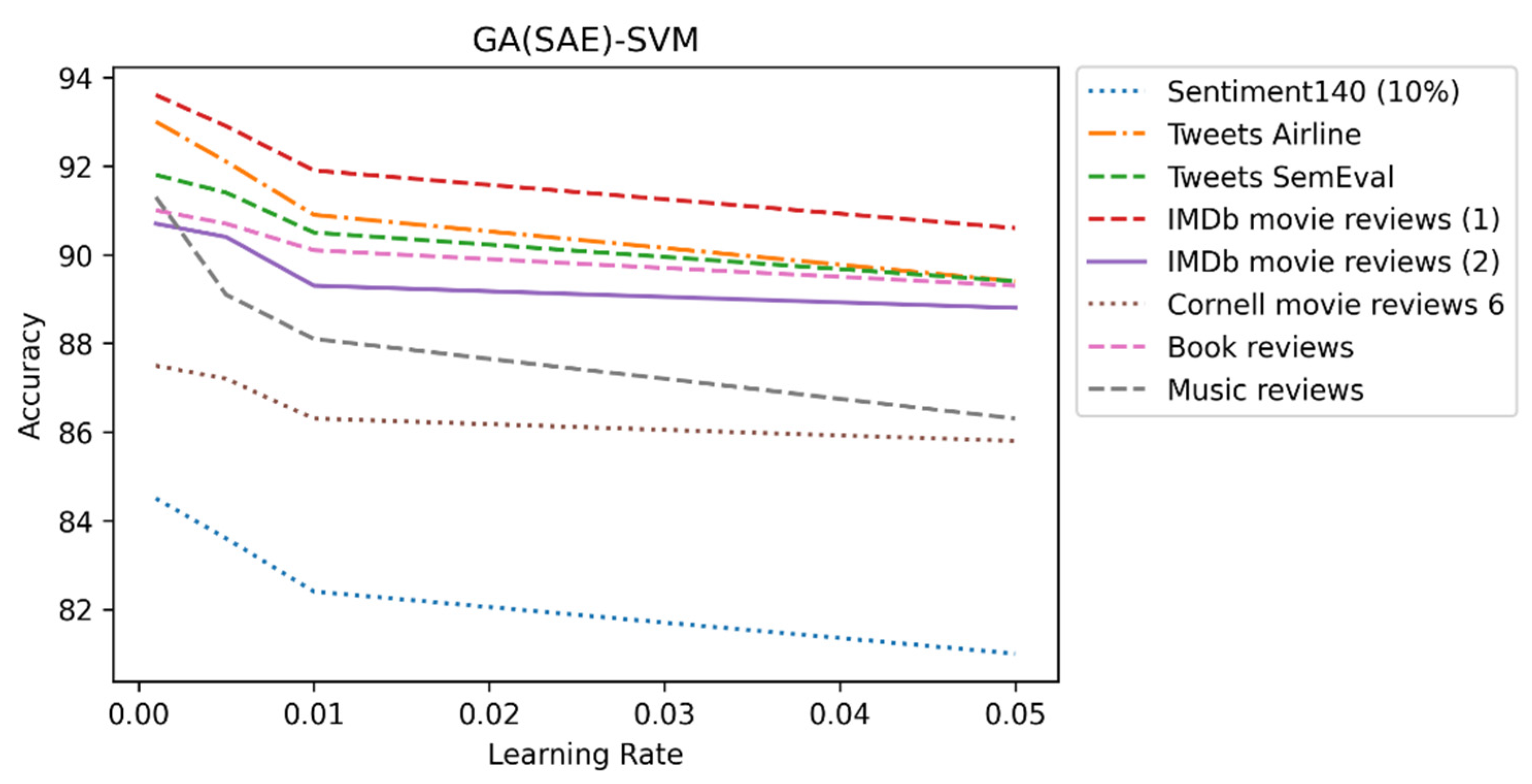
5.6.3. Learning Rate

Hyperparameters are interconnected in such a way that a change in the value of one parameter leads to changes in the values of other hyperparameters, which leads to an improvement in performance. Additionally, an optimal value of some hyperparameters depends on the values of other hyperparameters. For example, the learning rate is correlated with momentum, batch size, and L2 regularization. If the momentum decreases from 0.9 to 0.0, the learning rate increases 10-fold. In our research, GA optimized the learning rate for the SAE. We found that in each dataset, as the learning rate decreases, the accuracy increases. We established that 0.001 is the optimal learning rate. Figure 6 shows the effect of learning rate on accuracy.

5.6.4. Number of Epochs

Epochs play an essential role in model performance. If we train the model with few epochs, it leads to the underfitting of the data. By increasing the number of epochs, accuracy is increased for training. The longer the model is trained, the better it fits with the data. A time comes where the model is trained so well, and losses its capability to generalize. It shows good performance in training but not in testing. Our research model is trained with eight datasets for 100, 125, and 150 epochs. Figure 7 shows the accuracy of all datasets at different epochs.

6. Limitations

In this research, we used the GA for hyperparameter optimization of the SAE for the task of sentiment analysis. GA-based parameter optimization resulted in better accuracy in comparison to the baseline and state-of-the-art models. GAs have many advantages, such as the capacity to be easily modified for any problem, liability, parallelism, and their ability to handle large search spaces easily and robustly. However, they have some limitations. In GAs, premature convergence can occur. The problem of selecting many parameters, such as population size, mutation rate, and crossover rate. GAs must be linked with a local search, without which they may not find the global optimal solution and may remain in local optima. These disadvantages somehow limit the performance of the proposed model. Another limitation of this research is that we only used English datasets. The experimental settings of models for other languages are different, so these results cannot be generalized to any other language. We also considered only three classes of sentiment, however, sentiments can be divided into more categories. Moreover, in this research, we only considered textual data. In social media, posts contain emojis and images. Emojis and images also convey certain sentiments. It is worth mentioning that analyzing other forms of data can improve predictions.

7. Conclusions

In recent years, social networks, which have become an integral aspect of daily life, have gained greater significance. They are utilized in numerous industries today, including health, education, and academia. Utilization of social networks has exposed issues with social network analysis. Sentiment analysis, or opinion mining, which is one of the most well-known social network analysis concepts, is a field of study that analyzes people’s ideas, opinions, sentiments, ratings, attitudes, and feelings regarding assets such as products, services, organizations, individuals, topics, events, and attributes. In this paper, a novel model is proposed for fine-grained sentiment analysis. The proposed model uses GA-based SAE architecture with an SVM classifier. Hyperparameters of SAEs are optimized using GA. The SVM performed classification based on features extracted by SAEs. We tested the proposed model with eight sentiment analysis datasets that are publicly available, and compared the performance of the proposed model with random search and grid search optimizers. Results show that the proposed method achieved higher accuracy than other models. This study relied solely on reviews and tweets posted in English. We require social media datasets that include content from multiple languages in order to generalize our findings and conduct a global sentiment analysis. As a result, we aim to investigate algorithms that translate social media messages into languages other than English. Success in obtaining sentiment estimation in the future will be possible through the adoption of different metaheuristic techniques. Using hybrid variants of the relevant algorithms yields superior outcomes. Likewise, metaheuristic methods can be adapted for other social network analyses.

References

- Keenan, M.J.S. Advanced Positioning, Flow, and Sentiment Analysis in Commodity Markets Bridging Fundamental and Technical Analysis, 2nd ed.; Wiley: Hoboken, NJ, USA, 2018. [Google Scholar]
- Sohangir, S.; Wang, D.; Pomeranets, A.; Khoshgoftaar, T.M. Big Data: Deep Learning for financial sentiment analysis. J. Big Data 2018, 5, 3. [Google Scholar] [CrossRef]
- Jangid, H.; Singhal, S.; Shah, R.R.; Zimmermann, R. Aspect-based financial sentiment analysis using deep learning. In Proceedings of the Web Conference 2018, International World Wide Web Conferences Steering Committee, Lyon, France, 23 April 2018. [Google Scholar]
- Wang, G.; Yu, G.; Shen, X. The Effect of Online Investor Sentiment on Stock Movements: An LSTM Approach. Complexity 2020, 2020, 11. [Google Scholar] [CrossRef]
- Satapathy, R.; Cambria, E.; Hussain, A. Sentiment Analysis in the Bio-Medical Domain; Springer International Publishing AG: Basel, Switzerland, 2017. [Google Scholar] [CrossRef]
- Rajput, A. Natural language processing, sentiment analysis, and clinical analytics. In Innovation in Health Informatics; Academic Press: Cambridge, MA, USA, 2020; pp. 79–97. [Google Scholar]
- Malik, V.; Kumar, A. Sentiment analysis of twitter data using Naive Bayes algorithm. Int. J. Recent Innov. Trends Comput. Commun. 2018, 6, 120–125. [Google Scholar]
- Abid, F.; Alam, M.; Yasir, M.; Li, C. Sentiment analysis through recurrent variants latterly on convolutional neural network of Twitter. Futur. Gener. Comput. Syst. 2019, 95, 292–308. [Google Scholar] [CrossRef]
- Li, D.; Ahmed, K.; Zheng, Z.; Mohsan, S.A.H.; Alsharif, M.H.; Hadjouni, M.; Jamjoom, M.M.; Mostafa, S.M. Roman Urdu Sentiment Analysis Using Transfer Learning. Appl. Sci. 2022, 12, 10344. [Google Scholar] [CrossRef]
- Mhaskar, H.; Liao, Q.; Poggio, T. When and why are deep networks better than shallow ones? In Proceedings of the 2017 AAAI Conference on Artificial Intelligence, San Francisco, CA, USA, 4–9 February 2017. [Google Scholar]
- Schindler, A.; Lidy, T.; Rauber, A. Comparing shallow versus deep neural network architectures for automatic music genre classification. In Proceedings of the 9th Forum Media Technology (FMT2016), FMT, St. Pölten, Austria, 23–24 November 2016. [Google Scholar]
- Gupta, I.; Joshi, N. Enhanced twitter sentiment analysis using hybrid approach and by accounting local contextual se-mantic. J. Intell. Syst. 2019, 29, 1611–1625. [Google Scholar] [CrossRef]
- Alfrjani, R.; Osman, T.; Cosma, G. A Hybrid Semantic Knowledgebase-Machine Learning Approach for Opinion Mining. Data Knowl. Eng. 2019, 121, 88–108. [Google Scholar] [CrossRef]
- Dang, N.C.; Moreno-García, M.N.; De La Prieta, F. Sentiment Analysis Based on Deep Learning: A Comparative Study. Electronics 2020, 9, 483. [Google Scholar] [CrossRef]
- Srinidhi, H.; Siddesh, G.; Srinivasa, K. A hybrid model using MaLSTM based on recurrent neural networks with support vector machines for sentiment analysis. Eng. Appl. Sci. Res. 2020, 47, 232–240. [Google Scholar]
- Chauhan, U.A.; Afzal, M.T.; Shahid, A.; Abdar, M.; Basiri, M.E.; Zhou, X. A comprehensive analysis of adverb types for mining user sentiments on amazon product reviews. World Wide Web 2020, 23, 1811–1829. [Google Scholar] [CrossRef]
- Liu, B. Sentiment Analysis: Mining Opinions, Sentiments, and Emotions; Cambridge University Press: Cambridge, UK, 2015. [Google Scholar]
- Zhao, W.; Peng, H.; Eger, S.; Cambria, E.; Yang, M. Towards Scalable and Reliable Capsule Networks for Challenging NLP Applications; ACL: Stroudsburg, PL, USA, 2019; pp. 1549–1559. [Google Scholar]
- Duric, A.; Song, F. Feature selection for sentiment analysis based on content and syntax models. Decis. Support Syst. 2012, 53, 704–711. [Google Scholar] [CrossRef]
- Abbasi, A.; France, S.; Zhang, Z.; Chen, H. Selecting Attributes for Sentiment Classification Using Feature Relation Networks. IEEE Trans. Knowl. Data Eng. 2010, 23, 447–462. [Google Scholar] [CrossRef]
- Poria, S.; Chaturvedi, I.; Cambria, E.; Bisio, F. Sentic LDA: Improving on LDA with Semantic Similarity for Aspect-Based Sen-timent Analysis. In Proceedings of the 2016 International Joint Conference on Neural Networks (IJCNN), Vancouver, BC, Canada, 24–29 July 2016; pp. 4465–4473. [Google Scholar]
- Chaturvedi, I.; Ong, Y.-S.; Tsang, I.; Welsch, R.E.; Cambria, E. Learning word dependencies in text by means of a deep recurrent belief network. Knowl. Based Syst. 2016, 108, 144–154. [Google Scholar] [CrossRef]
- Basiri, M.E.; Kabiri, A. Words are important: Improving sentiment analysis in the persian language by lexicon refining. ACM Trans. Asian Low-Resour. Lang. Inf. Proc. 2018, 17, 1–18. [Google Scholar] [CrossRef]
- Basiri, M.E.; Ghasem-Aghaee, N.; Naghsh-Nilchi, A.R. Lexicon-based Sentiment Analysis in Persian. Curr. Future Dev. Artif. Intell. 2017, 30, 154–183. [Google Scholar] [CrossRef]
- Basiri, M.E.; Kabiri, A. HOMPer: A new hybrid system for opinion mining in the Persian language. J. Inf. Sci. 2019, 46, 101–117. [Google Scholar] [CrossRef]
- Abdar, M.; Basiri, M.E.; Yin, J.; Habibnezhad, M.; Chi, G.; Nemati, S.; Asadi, S. Energy choices in Alaska: Mining people’s per-ception and attitudes from geotagged tweets. Renew. Sustain. Energy Rev. 2020, 124, 109781. [Google Scholar] [CrossRef]
- Cambria, E.; Li, Y.; Xing, F.Z.; Poria, S.; Kwok, K. SenticNet 6: Ensemble Application of Symbolic and Subsymbolic AI for Sentiment Analysis. In Proceedings of the 29th ACM International Conference on Information and Knowledgement Management, Virtual Event, 19–23 October 2020; pp. 105–114. [Google Scholar]
- Zhang, L.; Ghosh, R.; Dekhil, M.; Hsu, M.; Liu, B. Combining Lexicon-Based and Learning-Based Methods for Twitter Sentiment Analysis; Technical Report HPL-2011; HP Laboratories: Palo Alto, CA, USA, 2011; Volume 89. [Google Scholar]
- Mudinas, A.; Zhang, D.; Levene, M. Combining lexicon and learning based approaches for concept-level sentiment analysis. In Proceedings of the First International Workshop on Issues of Sentiment Discovery and Opinion Mining, ACM, Beijing, China, 12–16 August 2012; p. 5. [Google Scholar]
- Ghiassi, M.; Lee, S. A domain transferable lexicon set for Twitter sentiment analysis using a supervised machine learning approach. Expert Syst. Appl. 2018, 106, 197–216. [Google Scholar] [CrossRef]
- Chikersal, P.; Poria, S.; Cambria, E.; Gelbukh, A.; Siong, C.E. Modelling public sentiment in twitter: Using linguistic patterns to enhance supervised learning. In Proceedings of the Computational Linguistics and Intelligent Text Processing, Cairo, Egypt, 14 April 2015; pp. 49–65. [Google Scholar] [CrossRef]
- Astya, P. Sentiment analysis: Approaches and open issues. In Proceedings of the International Conference on Computing, Communication and Automation (ICCCA), Greater Noida, India, 5 May 2017. [Google Scholar]
- Kaur, H.; Ahsaan, S.U.; Alankar, B.; Chang, V. A Proposed Sentiment Analysis Deep Learning Algorithm for Analyzing COVID-19 Tweets. Inf. Syst. Front. 2021, 23, 1417–1429. [Google Scholar] [CrossRef]
- Jnoub, N.; Al Machot, F.; Klas, W. A Domain-Independent Classification Model for Sentiment Analysis Using Neural Models. Appl. Sci. 2020, 10, 6221. [Google Scholar] [CrossRef]
- Ombabi, A.H.; Ouarda, W.; Alimi, A.M. Deep learning CNN–LSTM framework for Arabic sentiment analysis using textual information shared in social networks. Soc. Netw. Anal. Min. 2020, 10, 1–13. [Google Scholar] [CrossRef]
- Sanchez-Rada, J.F.S.; Iglesias, C.A. CRANK: A hybrid model for user and content sentiment classification using social context and community detection. Appl. Sci. 2020, 10, 1662. [Google Scholar] [CrossRef]
- Wang, Y.; Wang, M.; Xu, W. A Sentiment-Enhanced Hybrid Recommender System for Movie Recommendation: A Big Data Analytics Framework. Wirel. Commun. Mob. Comput. 2018, 2018, 9. [Google Scholar] [CrossRef]
- Baydogan, C.; Alatas, B. Sentiment analysis in social networks using social spider optimization algorithm. Teh. Vjesn. 2021, 28, 1943–1951. [Google Scholar]
- Akyol, S.; Alatas, B. Sentiment classification within online social media using whale optimization algorithm and social impact theory based optimization. Phys. A Stat. Mech. its Appl. 2020, 540, 123094. [Google Scholar] [CrossRef]
- Yildirim, S.; Yildirim, G.; Alatas, B. A new plant intelligence-based method for sentiment analysis: Chaotic sunflower optimization. Comput. Sci. 2021, 35–40. [Google Scholar] [CrossRef]
- Reeves, C.R. A genetic algorithm for flowshop sequencing. Comput. Oper. Res. 1995, 22, 5–13. [Google Scholar] [CrossRef]
- Houck, C.; Joines, J.; Kay, M. A Genetic Algorithm for Function Optimization: A Matlab Implementation. Ncsu-ie tr 1995, 95, 1–10. [Google Scholar]
- DeperlıOğlu, Ö.; Köse, U. Diagnosis of Diabetes Mellitus Using Deep Neural Network. In Proceedings of the 2018 2nd International Symposium on Multidisciplinary Studies and Innovative Technologies (ISMSIT), Ankara, Turkey, 19–21 October 2018; pp. 1–4. [Google Scholar]
- Stanley, K.O.; Miikkulainen, R. Evolving Neural Networks through Augmenting Topologies. Evol. Comput. 2002, 10, 99–127. [Google Scholar] [CrossRef]
- Bayer, J.; Wierstra, D.; Togelius, J.; Schmidhuber, J. Evolving Memory Cell Structures for Sequence Learning. In Proceedings of the International Conference on Artificial Neural Networks, Limassol, Cypros, 14–17 September 2009. [Google Scholar]
- Yao, X. Evolving Artificial Neural Networks. Proc. IEEE 1999, 87, 1423–1447. [Google Scholar]
- Ding, S.; Li, H.; Su, C.; Yu, J.; Jin, F. Evolutionary artificial neural networks: A review. Artif. Intell. Rev. 2011, 39, 251–260. [Google Scholar] [CrossRef]
- Xie, L.; Yuille, A. Genetic CNN. In Proceedings of the IEEE international conference on computer vision; 2017; pp. 1379–1388. [Google Scholar]
- Suganuma, M.; Shirakawa, S.; Nagao, T. A Genetic Programming Approach to Designing Convolutional Neural Network Architectures; GECCO: New York, NY, United States, 1 July 2017; pp. 497–504. [Google Scholar]
- Han, J.-H.; Choi, D.-J.; Park, S.-U.; Hong, S.-K. Hyperparameter Optimization Using a Genetic Algorithm Considering Verification Time in a Convolutional Neural Network. J. Electr. Eng. Technol. 2020, 15, 721–726. [Google Scholar] [CrossRef]
- Young, S.R.; Rose, D.C.; Karnowski, T.P.; Lim, S.; Patton, R.M. Optimizing deep learning hyper-parameters through an evolutionary algorithm. In Proceedings of the Workshop on Machine Learning in High-Performance Computing Environments-MLHPC ’15, Austin, TX, USA, 15 November 2015; pp. 1–5. [Google Scholar]
- Bansal, N.; Sharma, A.; Singh, R.K. An Evolving Hybrid Deep Learning Framework for legal document classification. Ing. Syst. Inf. 2019, 24, 425–4311. [Google Scholar]
- Bhandare, A.; Kaur, D. Designing Conventional Neural Network Using Genetic Algorithms. Int. J. Adv. Netw. Monit. Controls 2021, 6, 26–35. [Google Scholar] [CrossRef]
- Xiao, X.; Yan, M.; Basodl, S.; Ji, C.; Pan, Y. Efficient Hyperparameter Optimization in Deep Learning Using a Variable Length Genetic Algorithm. arXiv 2020, arXiv:2006.12703. [Google Scholar]
- Liashchynskyi, P.; Liashchynskyi, P. Grid Search, Random Search, Genetic Algorithm: A Big Comparison for NAS. arXiv 2019, arXiv:1912.06059. [Google Scholar]
- Vincent, P.; Larochelle, H.; Bengio, Y.; Manzagol, P. Extracting and composing robust features with denoising autoencoders. In Proceedings of the 25th International Conference on Machine Learning, Helsinki, Finland, 5 July 2008; pp. 1096–1103. [Google Scholar]
- Yoshua, B.; Pascal, L.; Dan, P.; Hugo, L. Greedy layer-wise training of deep networks. In Advances in Neural Information Processing Systems; MIT Press: Cambridge, MA, USA, 2007; pp. 153–160. [Google Scholar]
- Glorot, X.; Bordes, A.; Bengio, Y. Domain adaptation for large-scale sentiment classification: A deep learning approach. In Proceedings of the Twenty-Eight International Conference on Machine Learning, Bellevue, WA, USA, 28 June 2011–2 July 2011. [Google Scholar]
- Yoshua, B. Learning Deep Architectures For AI; Foundations and Trends in Machine Learning: Hanover, MA, USA, 2011; pp. 1–127. [Google Scholar]
- Silberer, C.; Lapata, M. Learning grounded meaning representations with autoencoders. In Proceedings of the 52nd Annual Meeting of the Association for Computational Linguistics, Baltimore, MD, USA, 23–25 June 2014; pp. 721–732. [Google Scholar]
- Whitley, D. A genetic algorithm tutorial. Statist. Comput. 1994, 4, 65–85. [Google Scholar] [CrossRef]
- Mitchell, M. Genetic algorithms: An overview. Complexity 1995, 1, 31–39. [Google Scholar] [CrossRef]
- Jebari, K.; Madiafi, M. Selection methods for genetic algorithms. Int. J. Emerg. Sci. 2013, 3, 333–344. [Google Scholar]
- Applegate, D.; Bixby, R.; Chvátal, V.; Cook, W. Implementing the Danting Fulkerman-Johnson Algorithm for Large Traveling Salesman Problems. Math. Program. 2003, 97, 91–98. [Google Scholar] [CrossRef]
- Yun, Y.; Gen, M. Performance analysis of adaptive genetic algorithms with fuzzy logic and heuristics. Fuzzy Optim. Decis. Mak. 2003, 2, 161–175. [Google Scholar] [CrossRef]
- Haupt, R.L.; Haupt, S.E. Practical Genetic Algorithms; Wiley: State College, PA, USA, 2004; pp. 123–190. [Google Scholar]
- Carr, J. An Introduction to Genetic Algorithms; Senior Project; MIT Press: Cambridge, MA, USA, 2014; Volume 1, p. 7. [Google Scholar]
- Chen, L.-S.; Liu, C.-H.; Chiu, H.-J. A neural network based approach for sentiment classification in the blogosphere. J. Inf. 2011, 5, 313–322. [Google Scholar] [CrossRef]
- Hastie, T.; Tibshirani, R.; Friedman, J. The Elements of Statistical Learning; Springer: New York, NY, USA, 2001. [Google Scholar]
- Tsytsarau, M.; Palpanas, T. Survey on mining subjective data on the web. Data Min. Knowl. Discov. 2012, 24, 478–514. [Google Scholar] [CrossRef]
- Haykin, S. Neural Networks: A Comprehensive Foundation, 2nd ed.; Prentice Hall: Upper Saddle River, NJ, USA, 1998. [Google Scholar]
- Horváth, G. Neural networks in measurement systems. In Advances in Learning Theory: Methods, Models and Applications; IOS Press: Leuven, Belgium, 2003; pp. 375–402. [Google Scholar]
- Mikolov, T.; Chen, K.; Corrado, G.S.; Dean, J.A. Computing Numeric Representations of Words in A High-Dimensional Space. U.S. Patent No. 9,037,464, 19 May 2015. [Google Scholar]
- Rehman, A.U.; Malik, A.K.; Raza, B.; Ali, W. A Hybrid CNN-LSTM Model for Improving Accuracy of Movie Reviews Sentiment Analysis. Multimed. Tools Appl. 2019, 78, 26597–26613. [Google Scholar] [CrossRef]
- Banic, N.; Elezovic, N. TVOR: Finding Discrete Total Variation Outliers Among Histograms. IEEE Access 2020, 9, 1807–1832. [Google Scholar] [CrossRef]
- Jang, B.; Kim, M.; Harerimana, G.; Kang, S.-U.; Kim, J.W. Bi-LSTM model to increase accuracy in text classification: Com-bining Word2vec CNN and attention mechanism. Appl. Sci. 2020, 10, 5841. [Google Scholar] [CrossRef]
- Kaynar, O.; Aydin, Z.; Görmez, Y. Comparison of feature reduction methods with deepautoencoder machine learning in sentiment analysis. Int. J. Inform. Technol. 2017, 10, 319–326. [Google Scholar] [CrossRef][Green Version]
- Han, K.-X.; Chien, W.; Chiu, C.-C.; Cheng, Y.-T. Application of Support Vector Machine (SVM) in the Sentiment Analysis of Twitter DataSet. Appl. Sci. 2020, 10, 1125. [Google Scholar] [CrossRef]
- Sentiment140-A Twitter Sentiment Analysis Tool. Available online: https://help.senti-ment140.com/site-functionality (accessed on 10 December 2020).
- Twitter US Airline Sentiment. Available online: https://www.kaggle.com/crowdflower/twitter-airline-sentiment (accessed on 10 December 2020).
- International Workshop on Semantic Evaluation. 2017. Available online: https://alt.qcri.org/semeval2017/ (accessed on 10 December 2020).
- Large Movie Review Dataset. Available online: https://ai.stanford.edu/∼7amaas/data/sen-timent/ (accessed on 10 December 2020).
- Bag of Words Meets Bags of Popcorn. Available online: https://www.kaggle.com/c/word2vec-nlp-tutorial/data?select=labeledTrainData.tsv.zip (accessed on 10 December 2020).
- Cornell CIS Computer Science. Available online: https://www.cs.cornell.edu/people/pabo/movie-review-data/ (accessed on 10 December 2020).
- Multi-domain Sentiment Dataset. Available online: https://www.cs.jhu.edu/∼mdredze/datasets/sentiment/ (accessed on 10 December 2020).
- Duan, X.; Ji, T.; Qian, W. Twitter US Airline Recommendation Prediction; Stanford University: Stanford, CA, USA, 2016; p. cs229. [Google Scholar]
- Maltoudoglou, L.; Paisios, A.; Papadopoulos, H. BERT-based conformal predictor for sentiment analysis. In Proceedings of the 2020 Conformal and Probabilistic Prediction and Applications, PMLR, Verona, Italy, 9–11 September 2020. [Google Scholar]
- Yang, Z.; Dai, Z.; Yang, Y.; Jaime, C.; Russ, R.S.; Quoc, V.L. Xlnet: Generalized autoregressive pretraining for language understanding. arXiv 2019, arXiv:1906.08237. [Google Scholar]
- Dang, C.N.; Moreno-García, M.N.; De la Prieta, F. Hybrid Deep Learning Models for Sentiment Analysis. Complexity 2021, 2021, 9986920. [Google Scholar] [CrossRef]
- Baziotis, C.; Pelekis, N.; Doulkeridis, C. Datastories at semeval-2017 task 4: Deep lstm with attention for messagelevel and topic-based sentiment analysis. In Proceedings of the 11th International Workshop on Semantic Evaluation (SemEval-2017), Vancouver, BC, Canada, 3–4 August 2017. [Google Scholar]
- Cliche, M. Bb_twtr at semeval-2017 task 4: Twitter sentiment analysis with CNNs and LSTMs. In Proceedings of the 11th International Workshop on Semantic Evaluation (SemEval-2017), Vancouver, BC, Canada, 3–4 August 2017. [Google Scholar]
- McCann, B.; Bradbury, J.; Xiong, C.; Socher, R. Learned in translation: Contextualized word vectors. In Proceedings of the 31st International Conference on Neural Information Processing Systems, Long Beach, CA, USA, 4–9 December 2017. [Google Scholar]
- Maulana, R.; Rahayuningsih, P.A.; Irmayani, W.; Saputra, D.; Jayanti, W.E. Improved accuracy of sentiment analysis movie review using support vector machine based information gain. In Proceedings of the International Conference on Advanced Information Scientific Development (ICAISD), West Java, Indonesia, 7 August 2020; IOP Publishing: Bristol, UK, 2020. [Google Scholar]
- Uribe, D. Domain adaptation in sentiment classification. In Proceedings of the 2010 Ninth International Conference on Machine Learning and Applications, IEEE, Washington, DC, USA, 12–14 December 2010. [Google Scholar]