An Effective Rainfall–Ponding Multi-Step Prediction Model Based on LSTM for Urban Waterlogging Points

Abstract

With the change in global climate and environment, the prevalence of extreme rainstorms and flood disasters has increased, causing serious economic and property losses. Therefore, accurate and rapid prediction of waterlogging has become an urgent problem to be solved. In this study, Jianye District in Nanjing City of China is taken as the study area. The time series data recorded by rainfall stations and ponding monitoring stations from January 2015 to August 2018 are used to build a ponding prediction model based on the long short-term memory (LSTM) neural network. MSE (mean square error), MAE (mean absolute error) and MSLE (mean squared logarithmic error) were used as loss functions to conduct and train the LSTM model, then three ponding prediction models were built, namely LSTM (mse), LSTM (mae) and LSTM (msle), and a multi-step model was used to predict the depth of ponding in the next 1 h. Using the measured ponding data to evaluate the model prediction results, we selected rmse (root mean squared error), mae, mape (mean absolute percentage error) and NSE (Nash–Sutcliffe efficiency coefficient) as the evaluation indicators. The results showed that LSTM (msle) was the best model among the three models, with evaluation indicators as follows: rmse 5.34, mae 3.45, mape 53.93% and NSE 0.35. At the same time, we found that LSTM (mae) has a better prediction effect than the LSTM (mse) and LSTM (msle) models when the ponding depth exceeds 30 mm.

1. Introduction

With climate warming and accelerated urbanization, the frequency of extreme rainfall events has increased. Rainstorm flood has become one of the main natural disasters plaguing many cities in China, and has brought serious threats to human production, life and socio-economic activities [1,2,3]. From 16 to 21 July 2021, a rare and continuous heavy precipitation weather process occurred in Zhengzhou, and, as of 12:00 on August 2, the heavy flooding caused by heavy rain caused direct economic losses of CNY 114.269 billion, 302 deaths and 50 people missing [4,5,6]. As one of the important non-engineering measures for flood control and disaster reduction, waterlogging prediction plays a key supporting role in urban flood control and disaster reduction. Although the existing physically driven urban waterlogging model can reflect the characteristics of urban rainfall-ponding in a certain period, there are still problems such as inefficient calculation and complex modeling [7].

With the advent of the era of big data and artificial intelligence, the abundance of hydrological observation data and the improvement of computer computing power [8], the use of neural networks for deep learning in the computer field to solve the problem of waterlogging prediction has become the focus of attention [9,10,11]. Among many neural networks, recurrent neural network (RNN) has better performance in processing and predicting time series data [12], but it also has the problem of gradient disappearance or explosion, which easily leads to unsatisfactory prediction results [13]. The LSTM is a variant of RNN, which largely improves the ability to handle long-term dependence problems and can handle time-dependent data well [14].

At present, the LSTM method is being widely used in multivariable field of hydrology. Chen et al. [15] used the LSTM model to study the water level fluctuation and reservoir operation in Dongting Lake. Comparing the LSTM model with the SVM model and comprehensively examining the impact of the presence of the Three Gorges Dam on the water level of Dongting Lake, it was concluded that the deviation value of the LSTM model was much smaller than that of the SVM model and showed better results in the prediction of high water levels; Sudriani et al. [16] proposed a deep learning algorithm based on a recursive long-term and short-term memory neural network to predict the irrigation flow in the dry season in advance. By comparing the measured data of basin stations, the results show that the relative error is less than 10%. Hrnjica et al. [17] proposed a lake water level prediction model based on FFNN and LSTM, performed an error analysis of the model simulation effects and proved that the model was effective in predicting time series data. Miao et al. [18] adopted a deep neural network composed of a convolutional neural network and an LSTM recursive module. The network model improved the resolution and accuracy of the GCM precipitation prediction. Kratzert et al. [19] trained LSTM models using a large flow dataset and compared the LSTM model prediction results with the actual flows, and found that the LSTM model can be used to predict watershed flows [20]. Zhang et al. [21] discussed the applicability of LSTM in water level prediction in urban drainage pipelines. Hu et al. [22] compared the ability of LSTM and ANN in rainfall runoff, and the results showed that the prediction accuracy of LSTM was higher than that of ANN.

Combined with the research status, machine learning technology is mostly applied to river basins, and its application in urban hydrology needs to be strengthened. However, the LSTM method itself is very mature, and the interdisciplinary research of machine learning technology represented by LSTM and the waterlogging simulation field is worth extensive testing. Therefore, the Jianye District of Nanjing, located in southeast China, is taken as the study area. Combined with the rainfall and ponding monitoring data in the study area, a multi-step and multivariable ponding prediction model is established based on the LSTM method. The performance of three loss functions (MSE, MAE and MSLE) in the rainfall–ponding prediction model was compared, and the influence of rolling step on the prediction result of water accumulation in the next hour was also explored.

2. Rainfall Prediction Model Construction

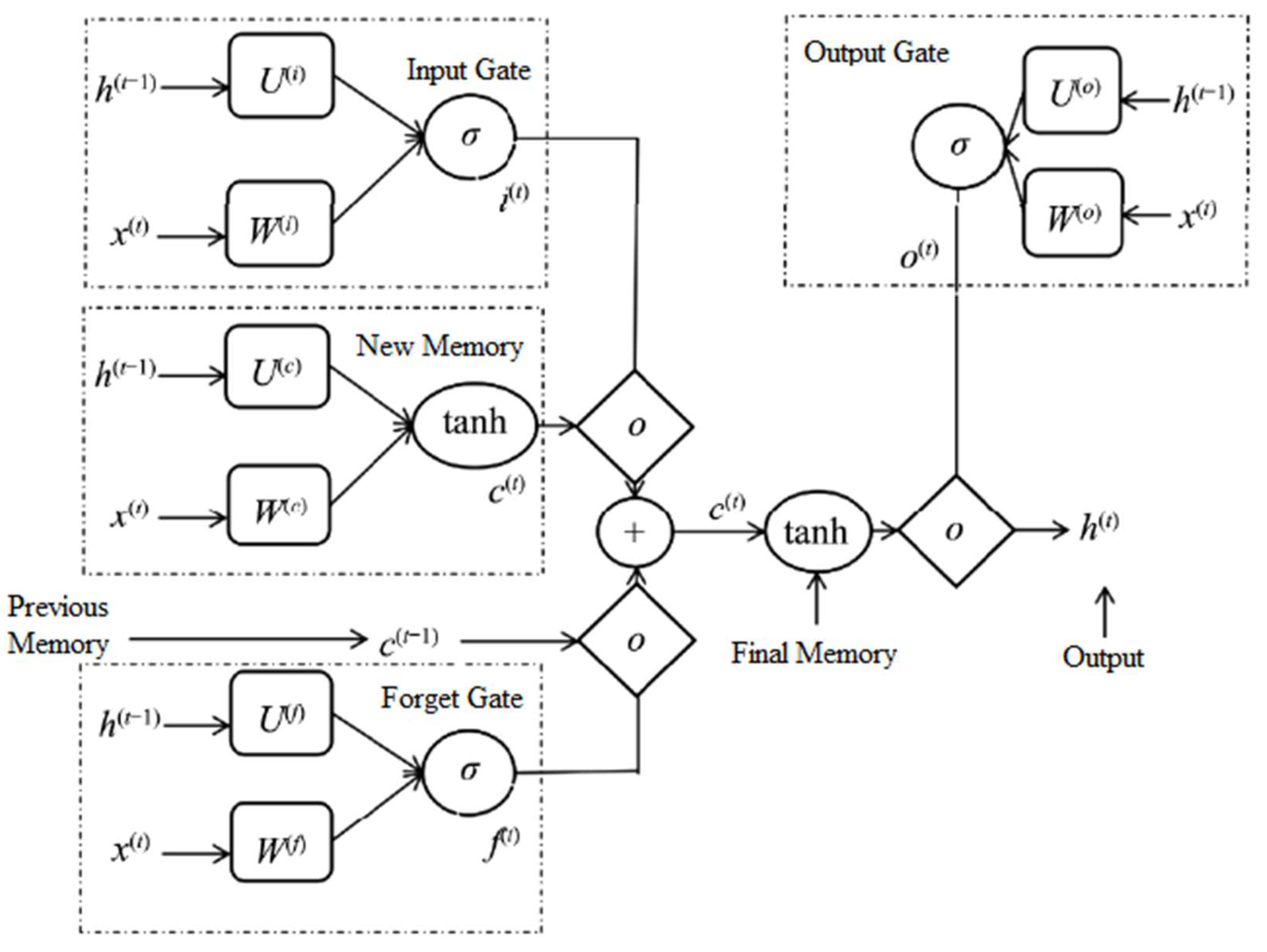
2.1. Modeling Principle

Deep learning is a concept introduced in recent years, which mainly refers to neural network models with more layers and neurons, including feedforward networks, feedback networks and self-organizing network models [23]. As one of the most popular variants of RNN, LSTM improves the problem of gradient disappearance in RNN through gate structure. LSTM cells contain three types of gates: input gates, which can be adaptively proportioned to the unit memory; forget gates, which mainly characterize the forgetting rate of the unit memory for a given input; and output gates, which mainly control the unit memory to influence the node output [24]. The LSTM structure is shown in Figure 1.

The output structure of LSTM outputs a value of 0 or 1 to the number in $c^{\left(t-1\right)}$ by reading $h^{\left(t-1\right)}$ and $x^{\left(t\right)}$, where “1” means keeping and “0” means discarding, as follows:

$$f^{\left(t\right)}=\sigma \left(W^{\left(f\right)} · \left[h^{\left(t-1\right)},x^{\left(t\right)}\right]+b^{\left(f\right)}\right)$$

(1)

where $h^{\left(t-1\right)}$ denotes the cell output at the previous moment and b denotes the corresponding bias term.

The input gate determines how much information is allowed to be added to the cell, and the cell state is updated through the information decision of the sigmoid layer in conjunction with the information generation of the $tanh$ layer [25]. The output gate determines which part of the information about the current cell state is output, still done through the sigmoid layer and the $tanh$ layer. The input gate steps are shown in Equations (2)–(4), and the output gate steps are shown in Equations (5) and (6):

$$i^{\left(t\right)}=\sigma \left(W^{\left(i\right)} · \left[h^{\left(t-1\right)},x^{\left(t\right)}\right]+b^{\left(i\right)}\right)$$

(2)

$${\tilde{c}}^{\left(t\right)}=tanh\left(W^{\left(c\right)} · \left[h^{\left(t-1\right)},x^{\left(t\right)}\right]+b^{\left(c\right)}\right)$$

(3)

$$c^{\left(t\right)}=f^{\left(t\right)} · c^{\left(t-1\right)}+i^{\left(t\right)} · {\tilde{c}}^{\left(t\right)}$$

(4)

$$o^{\left(t\right)}=\sigma \left(W^{\left(o\right)} · \left[h^{\left(t-1\right)},x^{\left(t\right)} \right]+b^{\left(o\right)}\right)$$

(5)

$$h^{\left(t\right)}=o^{\left(t\right)} · tanh\left(c^{\left(t\right)}\right)$$

(6)

where f, i, c and o denote the forget gate, input gate, cell state and output gate, respectively; $h^{\left(t\right)}$ denotes the output at the current moment; and σ and tanh denote the activation function sigmoid and hyperbolic tangent function, respectively [26].

2.2. Prediction Objectives

In this paper, through deep mining of historical rainfall data and ponding data, we construct a rainfall–ponding prediction model based on LSTM, design the model input–output structure as well as perform model parameter optimization, and achieve the goal of predicting future ponding processes at multiple time steps based on future rainfall prediction values through model calculations [19].

According to the experimental data, and the urban area production and confluence calculation method, the total duration from the beginning of the rainfall production process to the end of the surface confluence process is generally less than 4 h. Therefore, the prediction objective of this paper is to make multiple time-step predictions of the future 1 h ponding process using the past 4 h ponding process and the rainfall process at each relevant rainfall station, and combining the predicted values of the future 1 h rainfall process [27].

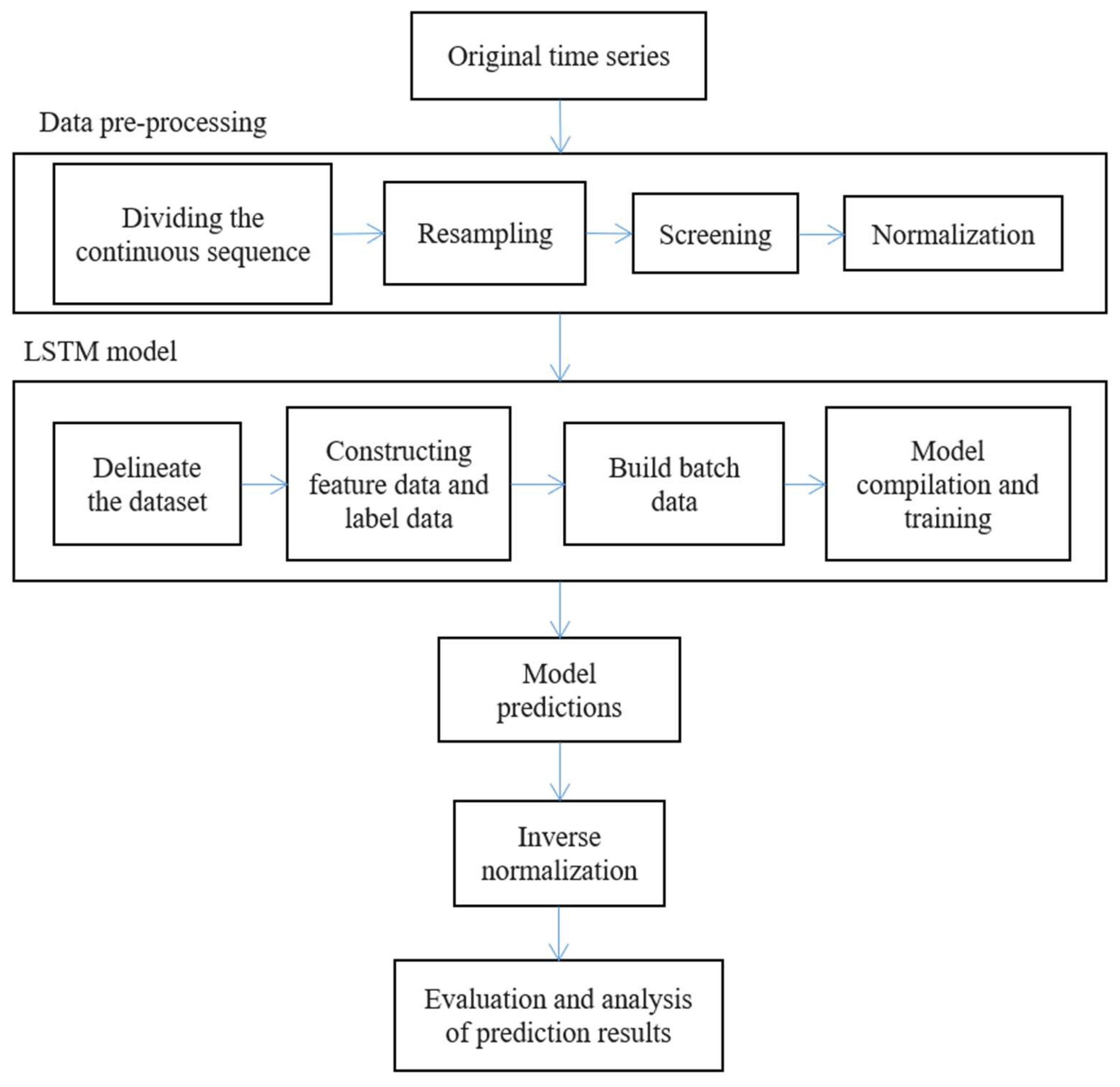
2.3. Model Framework

The framework of the rainfall–ponding prediction model is shown in Figure 2.

Data preprocessing plays a key role in the quality of model training results [28]. The raw rainfall data and ponding data are processed by resampling and normalization to obtain a time series suitable for model training [29]. Through data set partitioning, the time series are divided into a training set for model training, and a test set for model validation and evaluation. The original data were randomly divided into training set and test set according to the proportion of 80% and 20%.

According to the prediction objectives [30], the training and test sets are again divided into feature sets containing nonlinear features between multiple variables and label sets with the same prediction objectives by setting appropriate sliding windows. The models are compiled and trained separately by setting different loss functions to verify and evaluate the impact of the models trained by different compilation methods on the prediction results [31,32].

2.4. Optimization Algorithm in Model Compilation

Before using the deep learning model, it is generally necessary to abstract the problem to be solved mathematically, that is, define a loss function, and then use the optimization algorithm to minimize the loss function by changing the parameters of the deep learning model [33,34].

Due to its fast speed, small memory requirement and different adaptive learning rate for different parameters, the adaptive moment estimation (ADAM) optimization algorithm was selected in this study. MSE, MAE and MSLE were taken as loss functions to train the model and analyze their effects on the prediction results.

3. Case Study

3.1. Study Area and Data Sources

Jianye District is one of the six main urban areas of Nanjing, and the district boundary is determined as starting from Hanzhong Gate Avenue in the north, reaching the Qinhuai New River in the south, the External Qinhuai River in the east, and the Yangtze River midline in the west. The total area of the district is 80.87 km², and the topography is low in the south and high in the north, which is a Yangtze River floodplain landform unit [6]. Climatically, Jianye District belongs to the maritime climate zone with humid north subtropical climate zone and monsoon circulation, with significant monsoon, cold winter and hot summer, four distinct seasons, sufficient sunshine and abundant precipitation. Rainfall varies greatly between years and seasons, with obvious abundance and uneven rainfall distribution.

According to the prediction objectives, the time series data collected in this paper mainly includes two categories: the first category is rainfall data, which are all the recorded original rainfall data from January 2015 to August 2018 at the rainfall stations of Olympic Sports Center and Jiangxinzhou. The time interval of the original rainfall data is 1 h. The second category is the ponding monitoring data, which is recorded at the ponding survey point near the gas station on Jiqing Gate Avenue in the same period as the rainfall records, with a data interval of 5 min. The two categories of original time series data are generally partially continuous, and the data are continuous in a certain period of time when rainfall events occur.

3.2. Data Pre-Processing

Due to the different sources of the two types of raw data and the possible systematic bias caused by historical reasons, the raw data need to be pre-processed before the model training.

3.2.1. Continuous Series Segmentation

Both types of raw data are partially continuous and need to be divided into continuous series before interpolation. One hour is chosen as the criterion to determine whether the data is continuous or not. The adjacent moments in the original data with time interval more than one hour are intermittent points, and the time series between two intermittent points are continuous time series.

3.2.2. Resampling

According to the prediction target, this paper resamples the rainfall data and water depth data into a time series with 5 min as the time interval. The rainfall data is an hourly time series, so the interpolation method for its high frequency upsampling lacks practical significance, so this paper chooses to use the fill method to process the rainfall data. The short time interval of ponding depth data is suitable for downsampling the ponding time series by interpolation method. The commonly used interpolation methods are linear interpolation and cubic spline interpolation, etc. In order to avoid negative values in the interpolated time series, this paper chooses to use the linear method to process the ponding depth data.

3.2.3. Screening

At the moment t, the data are screened by using whether the sum of rainfall at each rainfall station is equal to 0 as the basis for determining whether the moment is a clear day or not, in order to properly eliminate potential systematic errors. The screening methods are: rain only and no screening.

3.2.4. Normalization

Because of the differences in the unit scale and order of magnitude of multivariate sensor data, it is easy to make the neural network difficult to converge and increase the training difficulty of the model, so this paper adopts the min–max standardization method to normalize the data.

$$x^{*}=\frac{x-x_{min}}{x_{max}-x_{min}}$$

(7)

where $x^{*}$ is the normalized data of a certain ponding factor; $x$ is the original data of a certain type of ponding factor; $x_{max}$ is the maximum value of a certain type of ponding factor; and $x_{min}$ is the minimum value of a certain type of ponding factor.

3.3. Model Training

3.3.1. Defining Labeled Data and Feature Data

In the pre-processed time series set, assuming that the total amount of data in each column is n, the labeled data set y is shown in Equation (8).

$$\mathrm{y}=\left({\mathrm{y}}_1,{ \mathrm{y}}_2,{ \mathrm{y}}_3, \dots ,{\mathrm{y}}_{\mathrm{n}}\right)$$

(8)

where y is the ponding dataset.

The feature data set X is shown in Equation (9).

$$\mathrm{X}=\left[\left({\mathrm{y}}_1,{ \mathrm{y}}_2,{ \mathrm{y}}_3, \dots ,{\mathrm{y}}_{\mathrm{n}}\right), \left({\mathrm{X}}_{11},{ \mathrm{X}}_{12},{ \mathrm{X}}_{13}, \dots ,{\mathrm{X}}_{1\mathrm{n}}\right),\left({\mathrm{X}}_{21},{ \mathrm{X}}_{22},{ \mathrm{X}}_{23}, \dots ,{\mathrm{X}}_{2\mathrm{n}}\right)\right]$$

(9)

where X is the rainfall dataset, X_1n is the rainfall dataset of the rainfall station of the Olympic Center and X_2n is the rainfall dataset of the rainfall station of Jiangxin island, where the training label dataset is denoted as y_train and the training feature dataset is denoted as X_train, the test label dataset is denoted as y_test and the test feature dataset is denoted as X_test.

3.3.2. Moving Sliding Window

According to the prediction target, the moving sliding window is set as shown in Equations (10) and (11).

$${\mathrm{y}}^{\mathrm{t}}=\left({\mathrm{y}}^{\mathrm{t}+1},{ \mathrm{y}}^{\mathrm{t}+2},{ \mathrm{y}}^{\mathrm{t}+3}, \dots ,{\mathrm{y}}^{\mathrm{t}+12}\right)$$

(10)

$${\mathrm{X}}^{\mathrm{t}}=\left[\begin{array}{c}\left({\mathrm{y}}^{\mathrm{t}-59},{ \mathrm{y}}^{\mathrm{t}-58},{ \mathrm{y}}^{\mathrm{t}-57}, \dots ,{\mathrm{y}}^{\mathrm{t}}\right), \left({\mathrm{X}}_1^{\mathrm{t}-59},{ \mathrm{X}}_1^{\mathrm{t}-58},{ \mathrm{X}}_1^{\mathrm{t}-57}, \dots ,{\mathrm{X}}_1^{\mathrm{t}+12}\right),\\ \left({\mathrm{X}}_2^{\mathrm{t}-59},{ \mathrm{X}}_2^{\mathrm{t}-58},{ \mathrm{X}}_2^{\mathrm{t}-57}, \dots ,{\mathrm{X}}_2^{\mathrm{t}+12}\right)\end{array}\right]$$

(11)

where t denotes the current moment, y^t is the label data and X^t is the feature data.

3.4. Hyperparameter Setting

The precision of LSTM model in predicting water depth is also related to the value of each hyperparameter. Hyperparameter refers to a group of optimal parameters that are searched and set in advance before the model starts training, which can better improve the accuracy and performance of the model. Sensitive hyperparameters in this study include: batch size, hidden layers, node numbers, dropout and epochs.

Set the initial values of the above parameters according to the recommended values in the relevant subject literature, and select the random search method to realize the automatic search optimization of the hyperparameters. The optimal superparameter combination is determined as follows:

Set the number of nodes in the input layer units = 256, the number of nodes in the output layer units = 32, and set two hidden layers with the number of nodes units = 128. To avoid model overfitting and to improve the model generalization ability, set dropout = 0.4 between the input layer to the first implied layer and dropout = 0.3 between the two implied layers. Set batch size = 256 and epochs = 30.

4. Evaluation of Prediction Results

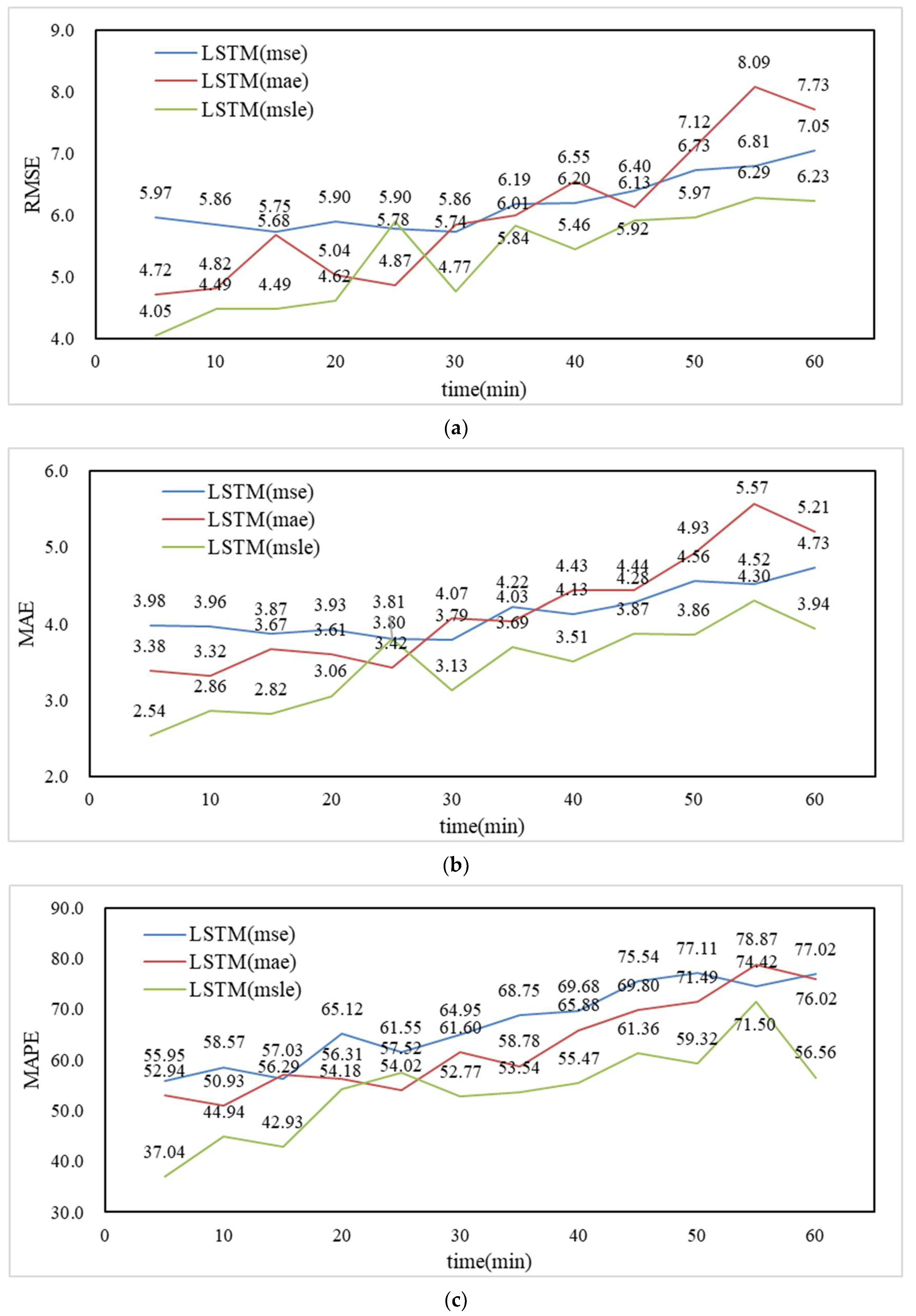
4.1. Prediction Accuracy Index

According to the “Hydrological Intelligence Forecasting Specification” and combined with the actual situation, RMSE, MAE, MAPE and NSE are selected in this paper as the prediction accuracy evaluation.

• Root mean squared error (RMSE)

The root mean square error is used to reflect the degree of deviation between the predicted and measured flood values, with smaller values indicating smaller deviations. The RMSE is calculated as shown in Equation (12).

$$\mathrm{RMSE}=\sqrt{\frac{1}{\mathrm{n}}{{\displaystyle \sum }}_{\mathrm{i}=1}^{\mathrm{n}}{\left[{\mathrm{y}}_{\mathrm{c}}\left(\mathrm{i}\right)-{\mathrm{y}}_0\left(\mathrm{i}\right)\right]}^2}$$

(12)

2.

Mean absolute error (MAE)

The mean absolute error reflects the degree of error between the predicted value and the measured value, and the smaller the value the closer the predicted value is to the measured value. MAE is calculated as shown in Equation (13).

$$\mathrm{MAE}=\frac{1}{\mathrm{n}}{{\displaystyle \sum }}_{\mathrm{i}=1}^{\mathrm{n}}\left|{\mathrm{y}}_{\mathrm{c}}\left(\mathrm{i}\right)-{\mathrm{y}}_0\left(\mathrm{i}\right)\right|$$

(13)

3.

Mean absolute percentage error (MAPE)

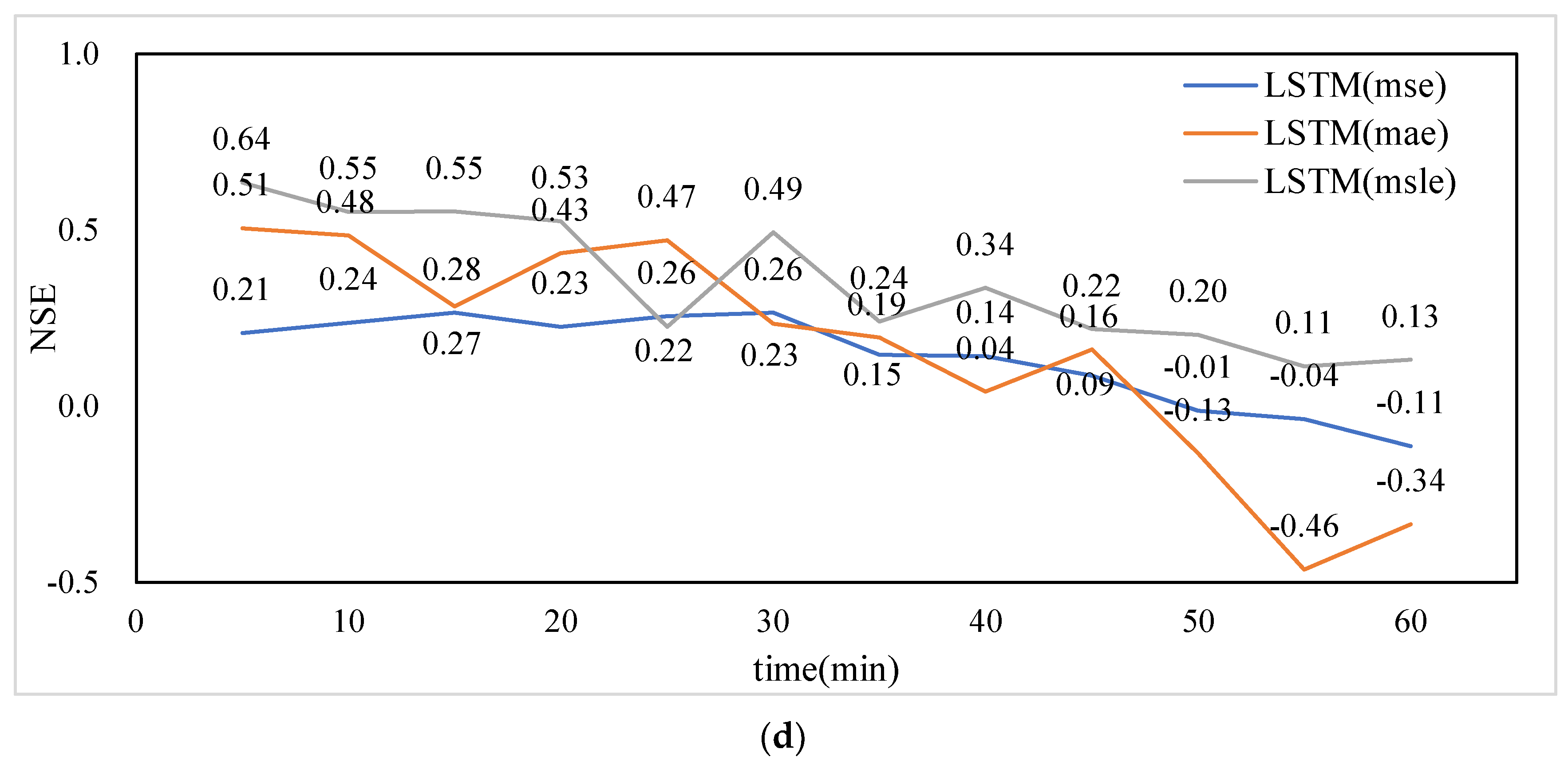
The mean absolute percentage error is used to reflect the error between predicted and measured values as a percentage of the measured values. A MAPE of 0% indicates a perfect model, while a MAPE greater than 100% indicates a poor model. MAPE is calculated as shown in Equation (14).

$$\mathrm{MAPE}=\frac{1}{\mathrm{n}}{{\displaystyle \sum }}_{\mathrm{i}=1}^{\mathrm{n}}\left|\frac{{\mathrm{y}}_{\mathrm{c}}\left(\mathrm{i}\right)-{\mathrm{y}}_0\left(\mathrm{i}\right)}{{\mathrm{y}}_0\left(\mathrm{i}\right)}\right|\times 100\%$$

(14)

4.

Nash–Sutcliffe efficiency coefficient (NSE)

$$\mathrm{NSE} =1-\frac{{{\displaystyle \sum }}_{\mathrm{i}=1}^{\mathrm{n}}{\left[{\mathrm{y}}_{\mathrm{c}}\left(\mathrm{i}\right)-{\mathrm{y}}_0\left(\mathrm{i}\right)\right]}^2}{{{\displaystyle \sum }}_{\mathrm{i}=1}^{\mathrm{n}}{\left[{\mathrm{y}}_{\mathrm{c}}\left(\mathrm{i}\right)-\overline{{\mathrm{y}}_0}\right]}^2}$$

(15)

The Nash–Sutcliffe efficiency coefficient is used to assess the predictive power of the hydrological model and takes values from negative infinity to 1. In the case of a perfect model with zero variance of the estimation error, the resulting NSE = 1; NSE = 0 indicates that the model has the same predictive power as the mean of the time series in terms of the sum of squared errors; if the variance of the estimation error of the modeled time series is significantly larger than the variance of the observations, NSE becomes negative.

In the above equation, ${\mathrm{y}}_{\mathrm{c}}\left(\mathrm{i}\right)$ is the predicted value, ${\mathrm{y}}_0\left(\mathrm{i}\right)$ is the measured value, $\overline{{\mathrm{y}}_0}$ is the mean of the measured value and n is the number of samples.

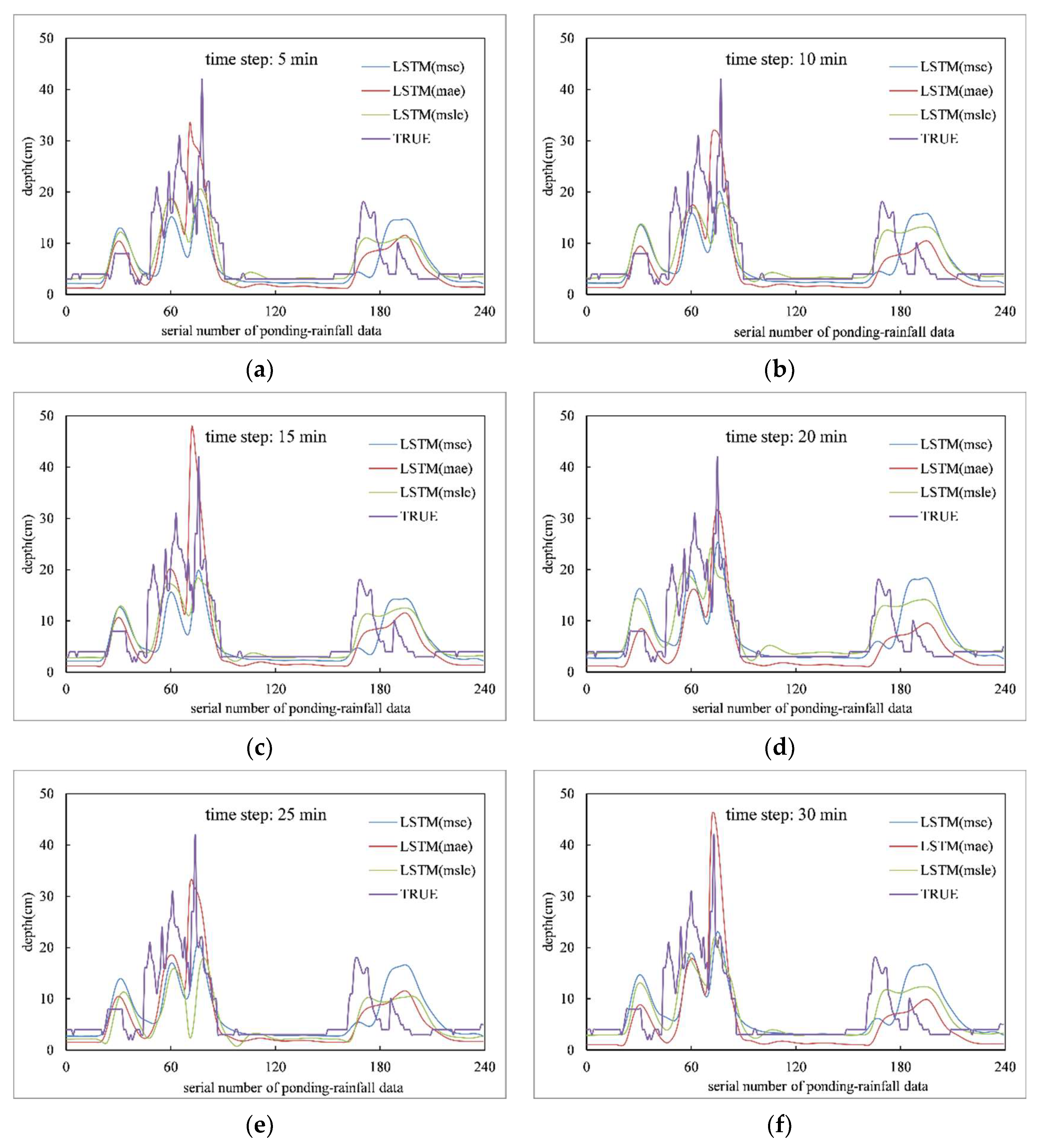
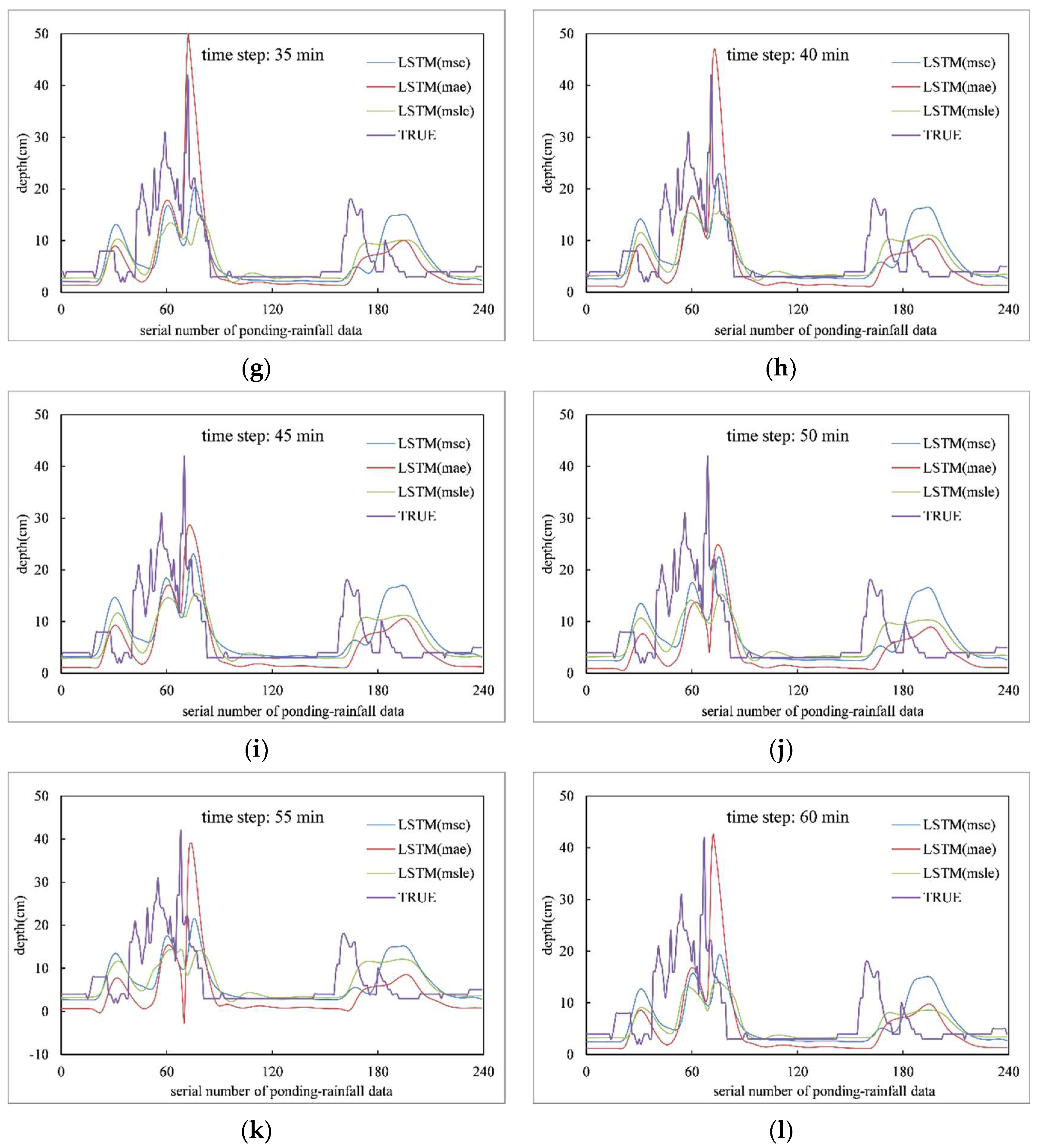
4.2. Analysis of Prediction Results

In this paper, rainfall data and ponding data from 1 August 2017 to 12 August 2017 are selected as the test set, with 240 sets of ponding–rainfall data, and the models are trained with MSE, MAE and MSLE as loss functions, denoted as LSTM (mse), LSTM (mae) and LSTM (msle). The prediction results for each time-step are shown in Figure 3.

According to Figure 3, the prediction results obtained from the LSTM models trained by the three loss functions are synchronous with the measured values in general, but all of them have different degrees of backward shift; the prediction results after 35 min in particular have a significant backward shift. For the prediction of the extreme values of ponding depth, LSTM (mae) predicted the extreme values over 40 mm close to the measured values, but the prediction for the general values of ponding depth (less than 30 mm) was poor; LSTM (mse) and LSTM (msle) predicted the general values better.

The prediction results of each model were evaluated by RMSE, MAE, MAPE and NSE for accuracy calculation, and the average value of prediction accuracy of each model at each time step is shown in Figure 4.

Compare the four precision indicators of the three models in pairs, and the accuracy comparison results are shown in

Table 1. Model accuracy comparison.

Time	LSTM (msle) vs. LSTM (mse)				LSTM (msle) vs. LSTM (mae)				LSTM (mse) vs. LSTM (mae)
	RMSE	MAE	MAPE (%)	NSE	RMSE	MAE	MAPE (%)	NSE	RMSE	MAE	MAPE (%)	NSE
5 min	−1.92	−1.43	−18.91	0.43	−0.67	−0.84	−15.90	0.13	1.25	0.59	3.01	−0.30
10 min	−1.37	−1.10	−13.64	0.31	−0.32	−0.46	−5.99	0.07	1.04	0.64	7.64	−0.25
15 min	−1.26	−1.06	−13.36	0.29	−1.19	−0.85	−14.11	0.27	0.06	0.20	−0.75	−0.02
20 min	−1.28	−0.87	−10.95	0.30	−0.42	−0.55	−2.13	0.09	0.86	0.32	8.82	−0.21
25 min	0.12	0.01	−4.03	−0.03	1.03	0.39	3.50	−0.25	0.91	0.38	7.52	−0.22
30 min	−0.97	−0.66	−12.18	0.23	−1.09	−0.94	−8.84	0.26	−0.12	−0.28	3.34	0.03
5–30 min average	−1.11	−0.85	−12.18	0.25	−0.45	−0.54	−7.25	0.10	0.67	0.31	4.93	−0.16
35 min	−0.35	−0.53	−15.21	0.09	−0.17	−0.34	−5.24	0.05	0.18	0.19	9.97	−0.05
40 min	−0.74	−0.62	−14.20	0.19	−1.10	−0.92	−10.41	0.29	−0.35	−0.30	3.79	0.10
45 min	−0.48	−0.41	−14.18	0.13	−0.21	−0.57	−8.43	0.06	0.27	−0.16	5.74	−0.07
50 min	−0.76	−0.70	−17.79	0.22	−1.15	−1.07	−12.17	0.34	−0.39	−0.37	5.62	0.12
55 min	−0.51	−0.21	−2.92	0.15	−1.79	−1.26	−7.37	0.58	−1.28	−1.05	−4.45	0.43
60 min	−0.82	−0.79	−20.46	0.24	−1.49	−1.27	−19.46	0.47	−0.67	−0.48	1.00	0.22
35–60 min average	−0.61	−0.54	−14.13	0.17	−0.99	−0.91	−10.51	0.30	−0.38	−0.36	3.61	0.12
full time average	−0.86	−0.70	−13.15	0.21	−0.72	−0.72	−8.88	0.20	0.15	−0.03	4.27	−0.02

.

According to Figure 4 and Table 1, LSTM (msle) is the model with the best accuracy indicators among the three models, in which the average RMSE is 5.34, MAE is 3.45, MAPE is 53.93% and NSE is 0.35. Compared with LSTM (mse) and LSTM (mae), full time average MAPE of LSTM (msle) decreased by 13.15% and 8.88%, respectively, and full time average NSE increased by 0.21 and 0.20, respectively.

The comparison results of LSTM (mse) and LSTM (mae) precision indicators show that the average RMSE, MAE and MAPE of LSTM (mse) in the first 30 min (the first 6 moments) were higher than those of LSTM (mae), and the NSE was relatively smaller, indicating that the prediction effect of LSTM (mae) was better than that of LSTM (mse) in the first 30 min; while the average RMSE, MAE and NSE of LSTM (mse) in the next 30 min (the last 6 moments) are slightly better than those of LSTM (mse).

5. Conclusions

In this paper, an effective rainfall–ponding prediction model is constructed based on LSTM for multi-step prediction of urban waterlogging. Relevant data from rainfall stations and ponding points in Nanjing from January 2015 to August 2018 were collected, and the models were trained with MSE, MAE and MSLE as loss functions and predicted the future 1 h ponding depths, and the following conclusions were drawn by calculating and comparing the prediction accuracy of each model:

• The LSTM fully exploits the nonlinear relationship between the rainfall data of each rainfall station and the ponding data of individual ponding survey points, and has a good multi-step prediction effect on the future ponding process.
• With the increase of time step, the prediction accuracy of each model decreases to different degrees, and 0–40 min in the future is the time range to achieve better prediction effect.
• The model trained with MSLE as the loss function has high prediction accuracy, but the prediction effect is not good in extreme or special conditions, while the model trained with MAE as the loss function can better predict the excessive ponding depth in special conditions.
• The limitation of our study lies in the fact that the number of positive samples in the data set is relatively small. In future research, we will set about extending the scale of the data set to build a predictive model with better performance. Meanwhile, we will consider other deep learning models, such as convolutional neural networks (CNNs), to improve the prediction of urban flood waterlogging depth.

References

1. Eduardo, A.A.; Felipe, F.B.; Reinaldo, J.M. A meta-heuristic based on simulated annealing for solving multiple-objective problems in simulation optimization. In Proceedings of the 2004 Winter Simulation Conference, Washington, DC, USA, 5–8 December 2004; pp. 508–513. [Google Scholar]
2. Zhongrun, X.; Jun, Y.; Ibrahim, D. A Rainfall-Runoff Model With LSTM-Based Sequence-to-Sequence Learning. Water Resour. Res. 2020, 56, e2019WR025326. [Google Scholar]
3. Zou, Q.; Xiong, Q.; Li, Q.; Yi, H.; Yu, Y.; Wu, C. A water quality prediction method based on the multi-time scale bidirectional long short-term memory network. Environ. Sci. Pollut. Res. Int. 2020, 27, 16853–16864. [Google Scholar] [CrossRef] [PubMed]
4. Tamiru, H.; Dinka, M.O. Application of ANN and HEC-RAS model for flood inundation mapping in lower Baro Akobo River Basin, Ethiopia. J. Hydrol. Reg. Stud. 2021, 36, 100855. [Google Scholar] [CrossRef]
5. Li, J.; Zhu, D.; Li, C. Comparative analysis of BPNN, SVR, LSTM, Random Forest, and LSTM-SVR for conditional simulation of non-Gaussian measured fluctuating wind pressures. Mech. Syst. Signal Process. 2022, 178, 109285. [Google Scholar] [CrossRef]
6. Yuhyeok, J.; Kyunghan, M.; Donghyuk, J.; Myoungho, S.; Manbae, H. Comparative study of the artificial neural network with three hyper-parameter optimization methods for the precise LP-EGR estimation using in-cylinder pressure in a turbocharged GDI engine. Appl. Therm. Eng. 2018, 149, 1324–1334. [Google Scholar]
7. Dimitri, P.S.; Avi, O. Data-driven modelling: Some past experiences and new approaches. J. Hydroinform. 2008, 10, 3–22. [Google Scholar]
8. Chen, Y.; Liu, T.; Ge, Y.; Xia, S.; Yuan, Y.; Li, W.; Xu, H. Examining social vulnerability to flood of affordable housing communities in Nanjing, China: Building long-term disaster resilience of low-income communities. Sustain. Cities Soc. 2021, 71, 102939. [Google Scholar] [CrossRef]
9. Hinton, G.E.; Osindero, S.; Teh, Y. A fast learning algorithm for deep belief nets. Neural Comput. 2006, 18, 1527–1542. [Google Scholar] [CrossRef]
10. Kumar, D.; Singh, A.; Samui, P.; Jha, R.K. Forecasting monthly precipitation using sequential modelling. Hydrol. Sci. J. 2019, 64, 690–700. [Google Scholar] [CrossRef]
11. Alipour, A.; Jafarzadegan, K.; Moradkhani, H. Global sensitivity analysis in hydrodynamic modeling and flood inundation mapping. Environ. Model. Softw. 2022, 152, 105398–105412. [Google Scholar] [CrossRef]
12. Wei, L.; Amin, K.; Clint, D. High temporal resolution rainfall–runoff modeling using long-short-term-memory (LSTM) networks. Neural Comput. Appl. 2020, 33, 1261–1278. [Google Scholar]
13. Nguyen, T.H.T.; Phan, Q.B. Hourly day ahead wind speed forecasting based on a hybrid model of EEMD, CNN-Bi-LSTM embedded with GA optimization. Energy Rep. 2022, 8, 53–60. [Google Scholar] [CrossRef]
14. Alberto, D.L.F.; Viviana, M.; Carolina, M. Hydrological Early Warning System Based on a Deep Learning Runoff Model Coupled with a Meteorological Forecast. Water-Sui. 2019, 11, 1808. [Google Scholar]
15. Chen, L.; Li, H.Q.; Lei, M.J.; Du, Q.Y. Dongting Lake water level forecast and its relationship with the Three Gorges Dam based on a long short-term memory network. Water 2018, 10, 1389. [Google Scholar]
16. Surdiani, Y.; Riewansyah, I.; Arustini, H. Long short term memory (LSTM) recurrent neural network (RNN) for discharge level prediction and forecast in Cimandiri river, Indonesia. IOP Conf. Ser. Earth Environ. Sci. 2019, 299, 1. [Google Scholar]
17. Hrnjica, B.; Bonacci, O. Lake level prediction using feed forward and recurrent neural networks. Water Resour. Manag. 2019, 33, 2471. [Google Scholar] [CrossRef]
18. Miao, Q.; Pan, B.; Wang, H.; Hsu, K.; Sorooshian, S. Improving monsoon precipitation prediction using combined convolutional and long short term memory neural network. Water 2019, 11, 977. [Google Scholar] [CrossRef]
19. Kratzert, F.; Klotz, D.; Brenner, C.; Schulz, K.; Herrnegger, M. Rainfall–runoff modelling using long short-term memory (LSTM) networks. Hydrol. Earth Syst. Sci. 2018, 22, 6005–6022. [Google Scholar] [CrossRef] [Green Version]
20. Xiaohui, Y.; Chen, C.; Xiaohui, L.; Yanbin, Y.; Rana, M.A. Monthly runoff forecasting based on LSTM–ALO model. Stoch. Environ. Res. Risk Assess. 2018, 32, 2199–2212. [Google Scholar]
21. Zhang, D.; Lindholm, G.; RAtnaweera, H. Use long short-term memory to enhance Internet of Things for combined sewer overflow monitoring. J. Hydrol. 2018, 556, 409–418. [Google Scholar] [CrossRef]
22. Hu, C.; Wu, Q.; Li, H.; Jian, S.; Li, N.; Lou, Z. Deep learning with a long short-term memory networks approach for rainfallrunoff simulation. Water 2018, 10, 1543. [Google Scholar] [CrossRef] [Green Version]
23. Zheng, W.; Liu, X.; Yin, L. Research on image classification method based on improved multi-scale relational network. PeerJ Comput. Sci. 2021, 7, e613. [Google Scholar] [CrossRef] [PubMed]
24. Chang, T.; Yu, H.; Wang, C.; Chen, A.S. Overland-gully-sewer (2D-1D-1D) urban inundation modeling based on cellular automata framework. J. Hydrol. 2021, 603, 1027001–1027016. [Google Scholar] [CrossRef]
25. Liu, B.; Wang, R.; Zhao, G.; Guo, X. Prediction of rock mass parameters in the TBM tunnel based on BP neural network integrated simulated annealing algorithm. Tunn. Undergr. Space Technol. Inc. Trenchless Technol. Res. 2020, 95, 103103–103114. [Google Scholar] [CrossRef]
26. Baek, S.; Pyo, J.; Chun, J.A. Prediction of Water Level and Water Quality Using a CNN-LSTM Combined Deep Learning Approach. Water 2020, 12, 3399–3411. [Google Scholar] [CrossRef]
27. Tambe, P.P. Selective Maintenance Optimization of a Multi-component System based on Simulated Annealing Algorithm. Procedia Comput. Sci. 2022, 200, 1412–1421. [Google Scholar] [CrossRef]
28. Shuai, G.; Yuefei, H.; Shuo, Z.; Jingcheng, H.; Guangqian, W.; Meixin, Z.; Qingsheng, L. Short-term runoff prediction with GRU and LSTM networks without requiring time step optimization during sample generation. J. Hydrol. 2020, 589, 125188–125198. [Google Scholar]
29. Wang, P.; Li, Y.; Yu, P.; Zhang, Y. The analysis of urban flood risk propagation based on the modified susceptible infected recovered model. J. Hydrol. 2021, 603, 127121–127136. [Google Scholar] [CrossRef]
30. Wu, X.; Liu, Z.; Yin, L.; Zheng, W.; Song, L.; Tian, J.; Yang, B.; Liu, S. A Haze Prediction Model in Chengdu Based on LSTM. Atmosphere 2021, 12, 1479. [Google Scholar] [CrossRef]
31. Wenjun, W.; Junli, L.; Zongyi, H.; Xinxin, Y.; Jie, Z.; Xiu, C.; Hongjiao, Q. Tracking spatio-temporal variation of geo-tagged topics with social media in China: A case study of 2016 hefei rainstorm. Int. J. Disaster Risk Reduct. 2020, 50, 101737–101752. [Google Scholar]
32. Lei, X.; Chen, W.; Panahi, M.; Falah, F.; Rahmati, O.; Uuemaa, E.; Kalantari, Z.; Ferreira, C.S.S.; Rezaie, F.; Tiefenbacher, J.P.; et al. Urban flood modeling using deep-learning approaches in Seoul, South Korea. J. Hydrol. 2021, 601, 126684–126696. [Google Scholar] [CrossRef]
33. Peng, J.; Zhang, J. Urban flooding risk assessment based on GIS- game theory combination weight: A case study of Zhengzhou City. Int. J. Disaster Risk Reduct. 2022, 77, 103080–103092. [Google Scholar] [CrossRef]
34. Bo, W.; Becky, P.Y.L.; Feng, Z.; Guangliang, X. Urban resilience from the lens of social media data: Responses to urban flooding in Nanjing, China. Cities 2020, 106, 102884–102896. [Google Scholar]
Figure 1. LSTM structure flow chart.
Applsci 12 12334 g001
Figure 2. Model framework.
Applsci 12 12334 g002
Figure 3. Predicted results of water depth at each time-step (al) are the prediction results of 5 min, 10 min, 15 min, 20 min, 25 min, 30 min, 35 min, 40 min, 45 min, 50 min, 55 min and 60 min.
Applsci 12 12334 g003aApplsci 12 12334 g003b
Figure 4. Evaluation of prediction accuracy at each moment measured by (a) RMSE, (b) MAE, (c) MAPE and (d) NSE.
Applsci 12 12334 g004aApplsci 12 12334 g004b