The Use of Asymmetric Polynomial Profiles for Planning a Smooth Trajectory
Abstract
1. Introduction
2. Materials and Methods
2.1. Asymmetric Acceleration Profile
- Should be in the interval t ∈ ⟨0,tend⟩;
- Will be asymmetric;
- Should be composed of two motion phases—the acceleration phase, for which s(2)(t) > 0 and the braking phase, for which s(2)(t) < 0, whereby the sequence of acceleration and braking phases is optional. The first motion phase is in the interval t ∈ ⟨0,k·tend⟩ but the other one is in the interval t ∈ (k·tend,tend⟩. The value of coefficient k, called the asymmetry coefficient, will be placed in the interval k ∈ (0,1);
- Should be tangent to the time axis for the first t = 0 and the last t = tend of the zero place.
2.2. Constraint of the Single Kinematic Quantity
- Determine the zero place of the function s(i+1)(t) in the interval t∈⟨0, tend⟩;
- Determine the value of the function s(i)(t) for successive zero places and then choose the one in which the function s(i)(t) archives the largest absolute value;
- Create a system of three equations in which there are compared:
- the dependence for the largest absolute value obtained in stage 2 with the given maximal value of the limited quantity smax(i);
- the dependence for the terminal position with the given terminal position;
- the dependence for the terminal velocity with the given terminal velocity;
- Solve the created system of equations by determining the coefficients of: polynomial p, asymmetry k and time of realization of the trajectory tend.
2.3. Constraint of Several Kinematic Quantities Simultaneously
3. Results
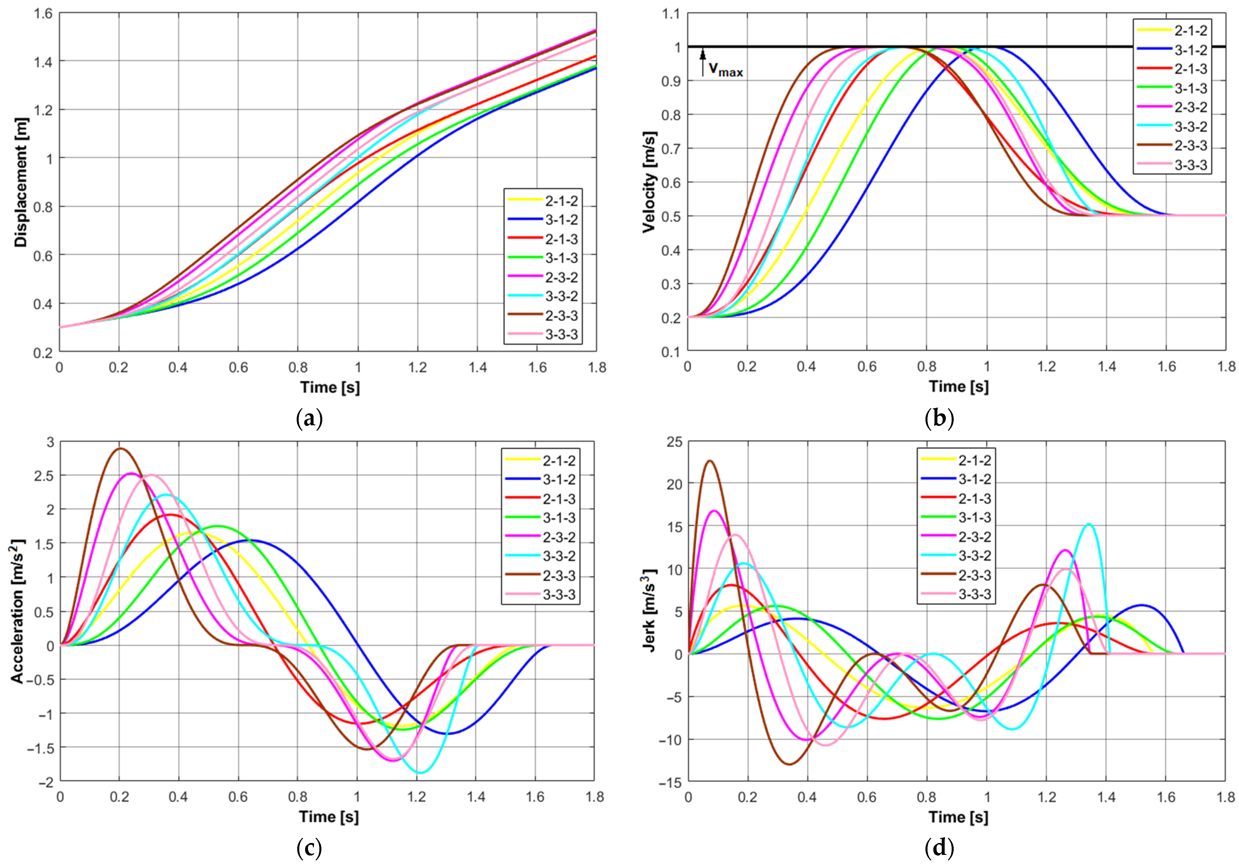
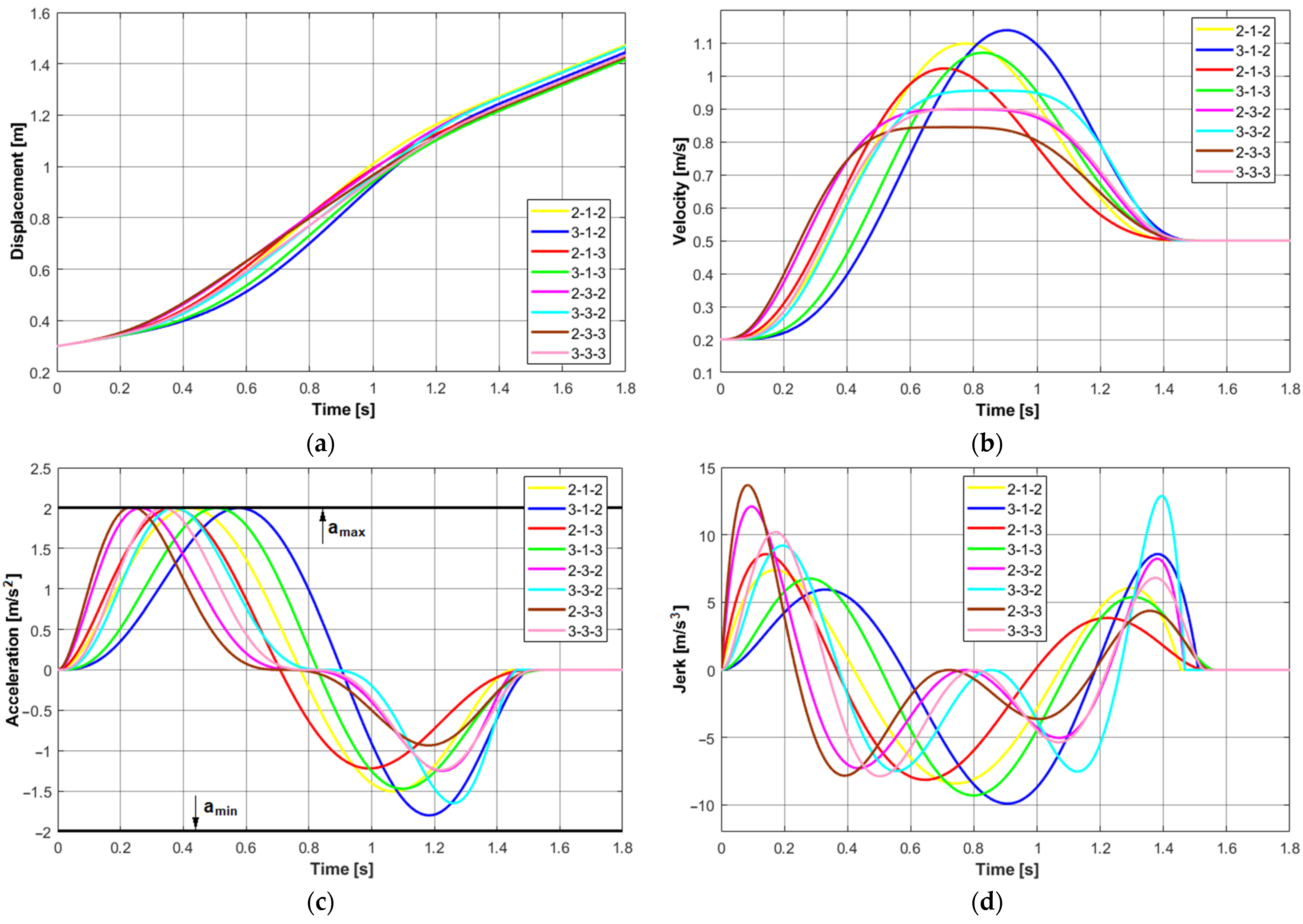
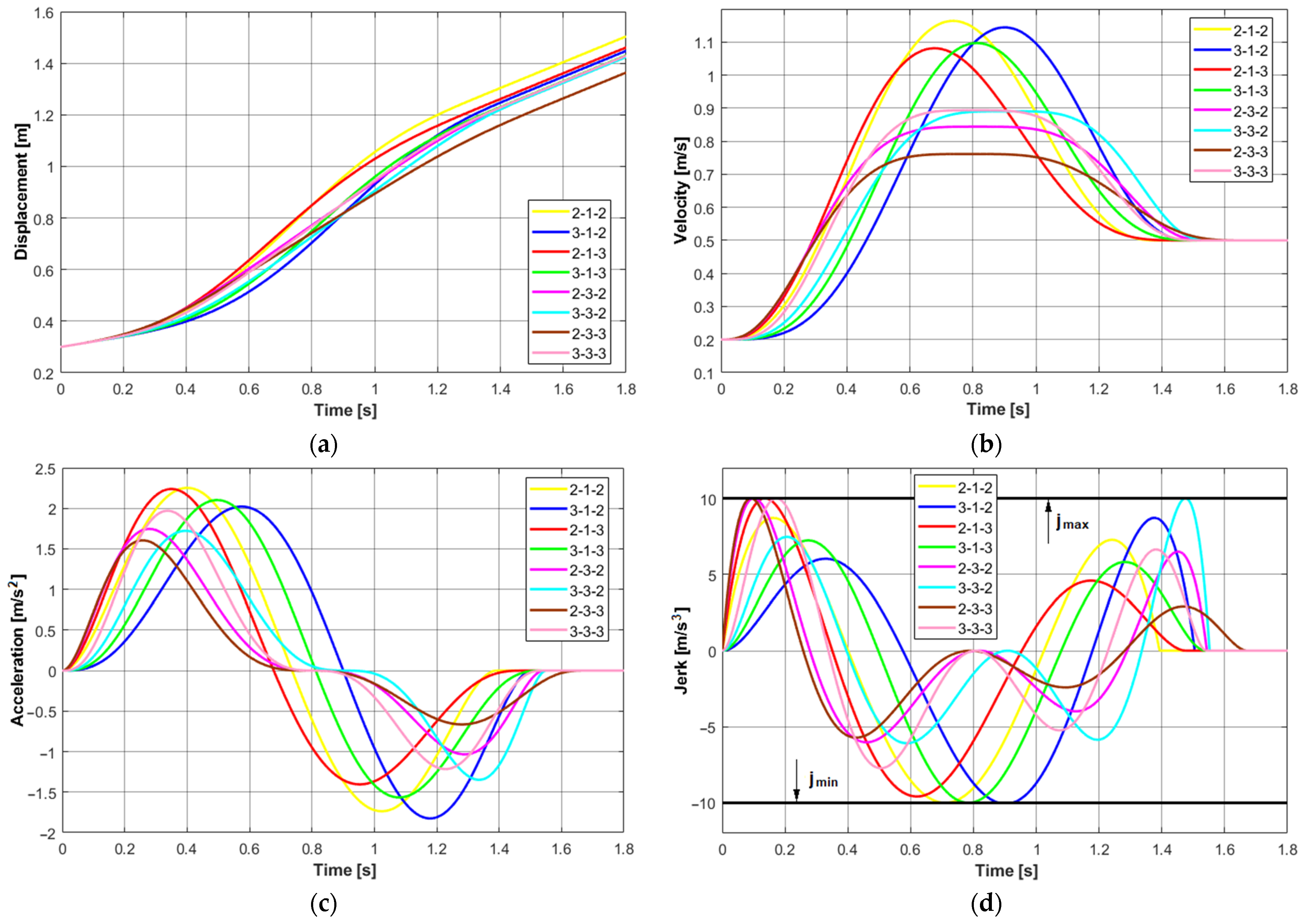
3.1. Results of the Simulation for a Single Constraint
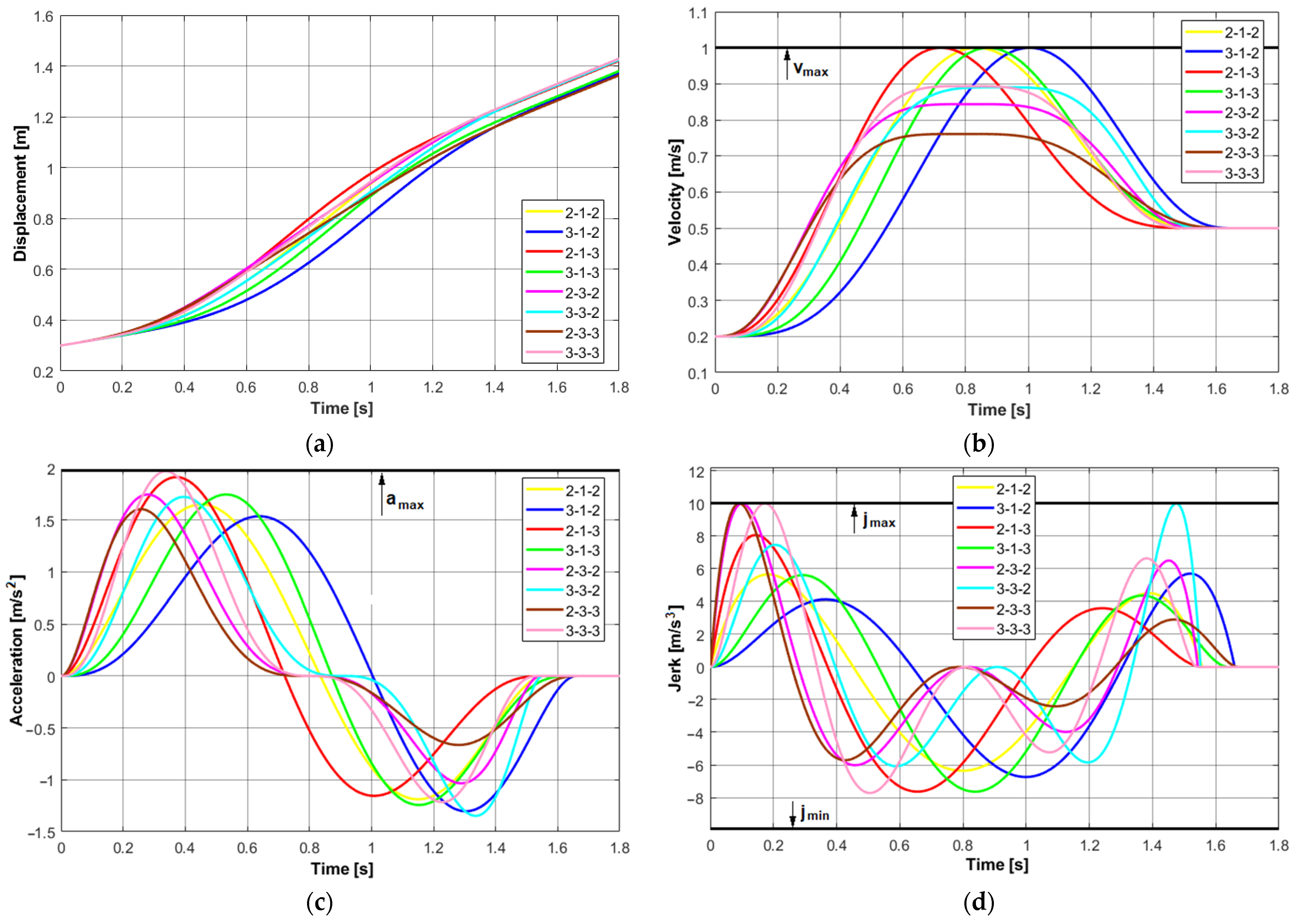
3.2. Simulation Results for a Few Kinematic Constraints
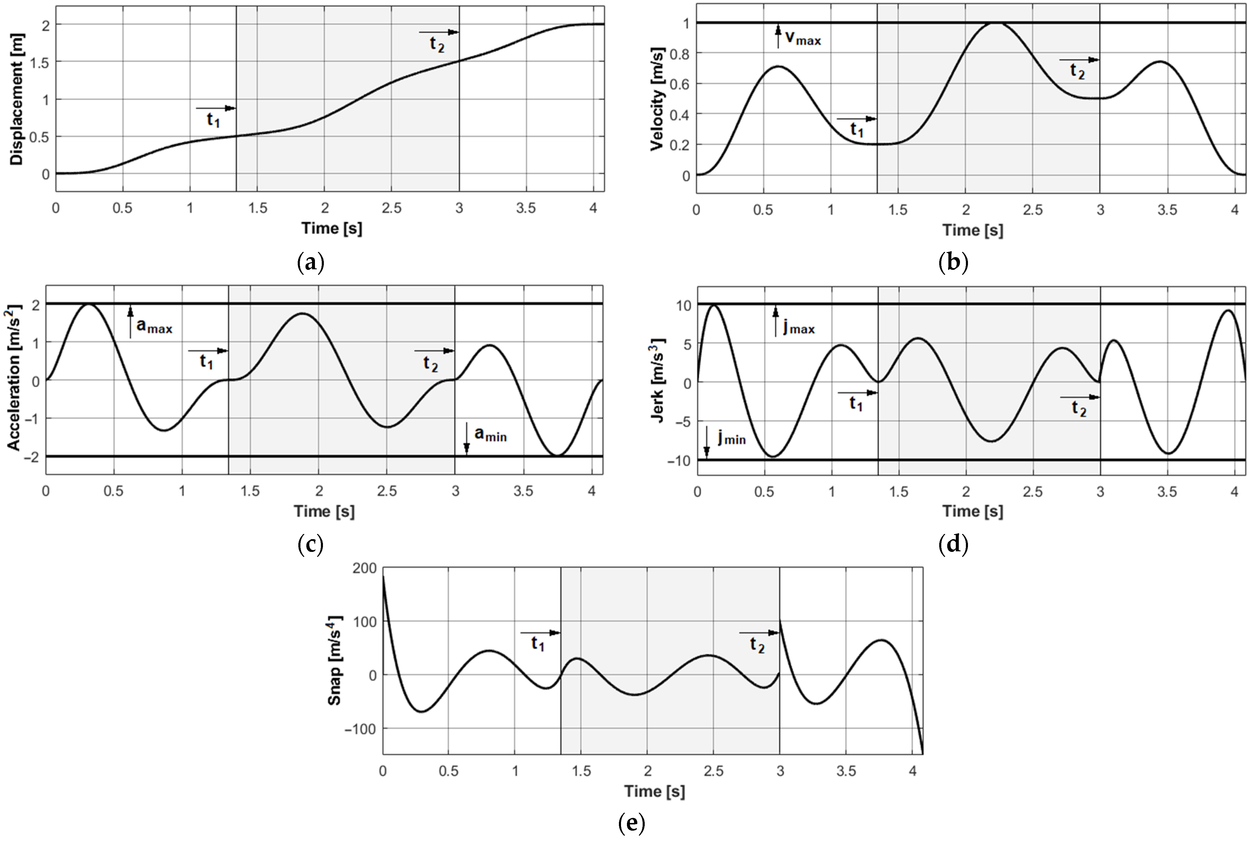
3.3. Concatenation of Polynomials
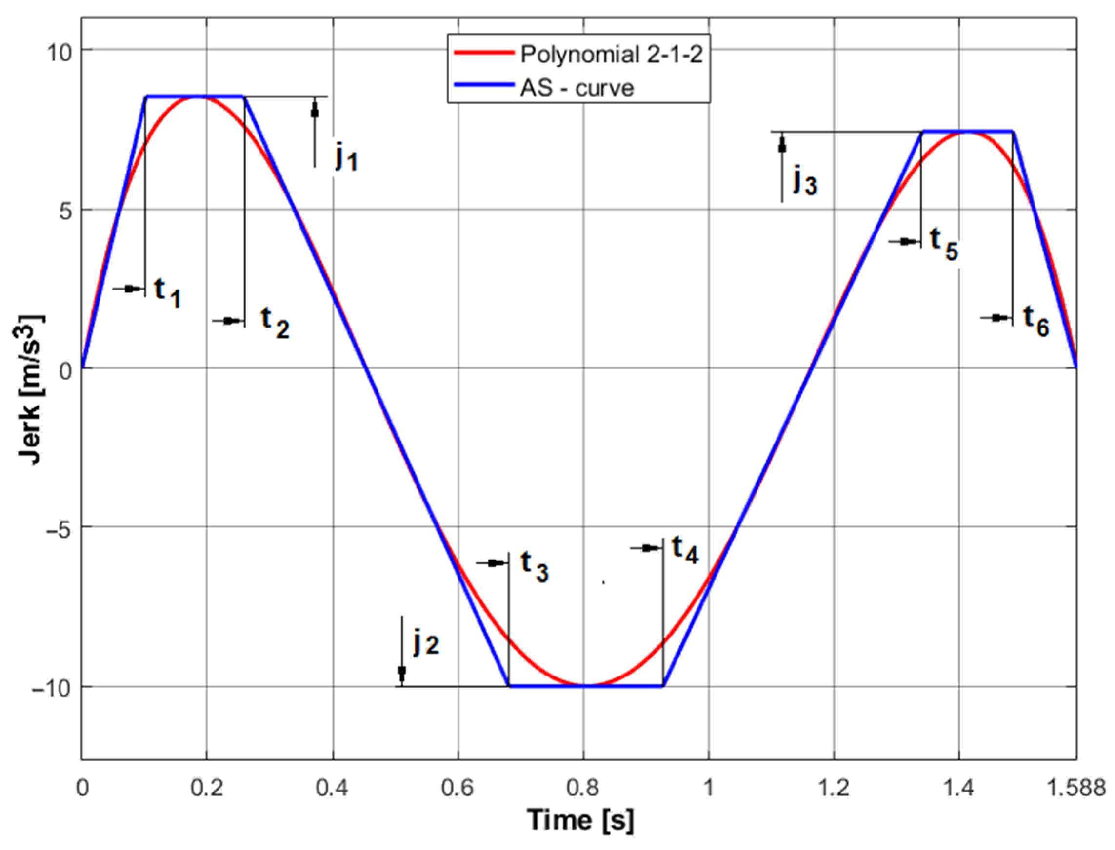
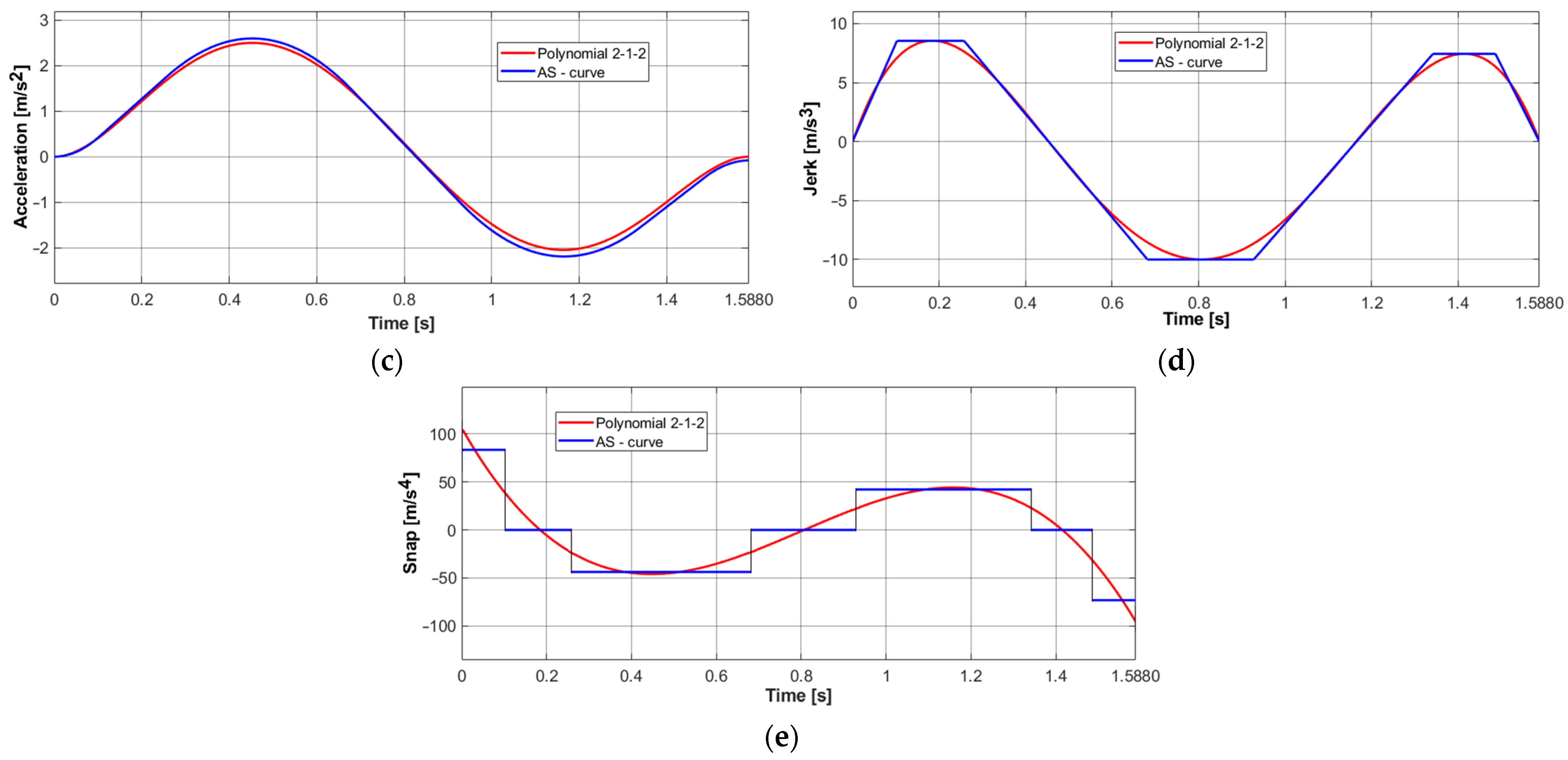
3.4. Comparison of the Polynomial Trajectory and the AS-Curve
4. Discussion
5. Conclusions
- The acceleration profiles presented in the paper, created using root multiplicities of polynomial, are simple in terms of mathematical description. Determination of other kinematic quantities based on them also does not cause computational difficulties.
- As a result of the use of asymmetric profiles, for which the assumed initial and final velocity values are arbitrary, it is possible to concatenate the analyzed polynomial profiles, allowing planning of trajectories with intermediate points.
- Application of all polynomials analyzed in the paper for the formation of motion trajectories passing through via-points, ensures continuity of acceleration and jerk in the whole motion range and using the polynomials 3-1-3 and 3-3-3, it is possible to obtain continuity of snap and at the same time its zero values for the time t = tbegin and t = tend.
- Exploitation of the analyzed polynomials enables planning the motion paths for which there can be fulfilled (except for the assumed constraints) additional requirements, including, e.g., the shortest time, minimal acceleration or jerk, etc.
- The possibility of introducing constraints on speed, acceleration and jerk can facilitate, already at the initial planning stage, the adaptation of the trajectory to, for example, the known movement capabilities of the kinematic chain and the properties of the drive system.
- The acceleration function along with easily derived displacement, velocity and jerk functions are ready-made motion patterns and can be used for trajectory planning: effectors of manipulators, toolheads of the CNC machines as well as mobile robots and autonomous vehicles.
Author Contributions
Funding
Institutional Review Board Statement
Informed Consent Statement
Data Availability Statement
Conflicts of Interest
Appendix A
References
- Biagiotti, L.; Melchiorri, C. Composition of elementary trajectories. In Trajectory Planning for Automatic Machines and Robots, 1st ed.; Springer: New York, NY, USA, 2009. [Google Scholar]
- Visioli, A. Trajectory planning of robot manipulators by using algebraic and trigonometric splines. Robotica 2000, 18, 611–631. [Google Scholar] [CrossRef]
- Dyllong, E.; Visioli, A. Planning and real-time modifications of a trajectory using spline techniques. Robotica 2003, 21, 475–482. [Google Scholar] [CrossRef]
- Saramago, S.F.P.; Ceccarelli, M. An optimum robot path planning with payload constraints. Robotica 2002, 20, 395–404. [Google Scholar] [CrossRef]
- Macfarlane, S.; Croft, E.A. Jerk-bounded manipulator trajectory planning: Design for real-time applications. IEEE Trans. Robot. Autom. 2003, 19, 42–52. [Google Scholar] [CrossRef]
- Kim, J.; Jin, M.; Park, S.H.; Chung, S.Y.; Hwang, M.J. Task Space Trajectory Planning for Robot Manipulators to Follow 3-D Curved Contours. Electronics 2020, 9, 1424. [Google Scholar] [CrossRef]
- Rew, K.H.; Ha, C.W.; Kim, K.S. A practically efficient method for motion control based on asymmetric velocity profile. Int. J. Mach. Tools Manuf. 2009, 49, 678–682. [Google Scholar] [CrossRef]
- Rew, K.H.; Kim, K.S. A Closed-Form Solution to Asymmetric Motion Profile Allowing Acceleration Manipulation. IEEE Trans. Ind. Electron. 2010, 57, 2499–2506. [Google Scholar] [CrossRef]
- Chen, Y.D.; Wei, H.X.; Sun, K.; Liu, M.; Wang, T.M. Algorithm for smooth S-curve federate profiling generation. Chin. J. Mech. Eng. 2011, 24, 237–247. [Google Scholar] [CrossRef]
- Ezair, B.; Tassa, T.; Shiller, Z. Planning high order trajectories with general initial and final conditions and asymmetric bounds. Int. J. Rob. Res. 2014, 33, 898–916. [Google Scholar] [CrossRef]
- Lee, A.Y.; Choi, Y. Smooth trajectory planning methods using physical limits. Proc. Inst. Mech. Eng. Part C J. Eng. Mech. Eng. Sci. 2015, 229, 2127–2143. [Google Scholar] [CrossRef]
- Li, H.Z. A jerk-constrained asymmetric motion profile for high-speed motion stages to reduce residual vibration. Int. J. Comput. Appl. Technol. 2016, 53, 149–156. [Google Scholar] [CrossRef]
- Fang, Y.; Hu, J.; Liu, W.H.; Shao, Q.Q.; Qi, J.; Peng, Y.H. Smooth and time-optimal S-curve trajectory planning for automated robots and machines. Mech. Mach. Theory 2019, 137, 127–153. [Google Scholar] [CrossRef]
- Alpers, B. On fast jerk–, acceleration– and velocity–restricted motion functions for online trajectory generation. Robotics 2021, 10, 25. [Google Scholar] [CrossRef]
- Alpers, B. On fast jerk-continuous motion functions with higher-order kinematic restrictions for online trajectory generation. Robotics 2022, 11, 73. [Google Scholar] [CrossRef]
- Choi, Y.K.; Park, J.H.; Kim, H.S.; Kim, J.H. Optimal trajectory planning and sliding mode control for robots using evolution strategy. Robotica 2000, 18, 423–428. [Google Scholar] [CrossRef]
- Constantinescu, D.; Croft, E.A. Smooth and time optimal trajectory planning for industrial manipulators along specified paths. J. Robot. Syst. 2000, 17, 233–249. [Google Scholar] [CrossRef]
- Red, E. A dynamic optimal trajectory generator for Cartesian Path following. Robotica 2000, 18, 451–458. [Google Scholar] [CrossRef]
- Lambrechts, P.; Boerlage, M.; Steinbuch, M. Trajectory planning and feedforward design for electromechanical motion systems. Control Eng. Pract. 2005, 13, 145–157. [Google Scholar] [CrossRef]
- Huang, P.; Xu, Y.; Liang, B. Global minimum-jerk trajectory planning of space manipulator. Int. J. Control Autom. Syst. 2006, 4, 405–413. [Google Scholar]
- Gasparetto, A.; Zanotto, V. A new method for smooth trajectory planning of robot manipulators. Mech. Mach. Theory. 2007, 42, 455–471. [Google Scholar] [CrossRef]
- Gasparetto, A.; Zanotto, V. A technique for time-jerk optimal planning of robot trajectories. Robot. Comput.-Integr. Manuf. 2008, 24, 415–426. [Google Scholar] [CrossRef]
- Gasparetto, A.; Zanotto, V. Optimal trajectory planning for industrial robots. Adv. Eng. Softw. 2010, 41, 548–556. [Google Scholar] [CrossRef]
- Nguyen, K.D.; Ng, T.C.; Chen, I.M. On algorithms for planning S-curve motion profiles. Int. J. Adv. Robot. Syst. 2008, 5, 99–106. [Google Scholar] [CrossRef]
- Biagiotti, L.; Melchiorri, C. FIR filters for online trajectory planning with time- and frequency-domain specifications. Control Eng. Pract. 2012, 20, 1385–1399. [Google Scholar] [CrossRef]
- Biagiotti, L.; Melchiorri, C. Trajectory generation via FIR filters: A procedure for time-optimization under kinematic and frequency constraints. Control Eng. Pract. 2019, 87, 43–58. [Google Scholar] [CrossRef]
- Fan, W.; Gao, A.S.; Yan, W.; Yuan, C.M. Interpolation of parametric CNC machining path under confined jounce. Int. J. Adv. Manuf. Technol. 2012, 62, 719–739. [Google Scholar] [CrossRef]
- Meligy, R.E.; Bassiuny, A.M.; Bakr, E.M.; Tantawy, A.A. A feasible minimum-time trajectory of robot manipulator. In Proceedings of the 9th International Symposium of Mechatronics and its Applications, Amman, Jordan, 9–11 April 2013; ISMA13. pp. 1–5. [Google Scholar]
- Wang, S.D.; Luo, X.; Xu, S.J.; Luo, Q.S.; Han, B.L.; Liang, G.H.; Jia, Y. A planning method for multi-axis point-to-point synchronization based on time constraints. IEEE Access 2020, 8, 85575–85604. [Google Scholar] [CrossRef]
- Wang, F.; Zhijun Wu, Z.; Bao, T. Time-Jerk optimal Trajectory Planning of Industrial Robots Based on a Hybrid WOA-GA Algorithm. Processes 2022, 10, 1014. [Google Scholar] [CrossRef]
- Wu, Z.; Chen, J.; Bao, T.; Wang, J.; Zhang, L.; Xu, F. A Novel Point-to-Point Trajectory Planning Algorithm for Industrial Robots Based on a Locally Asymmetrical Jerk Motion Profile. Processes 2022, 10, 728. [Google Scholar] [CrossRef]
- Zhao, J.; Bai, S.X. The study of coordinated manipulation of two redundant robots with elastic joints. Mech. Mach. Theory 2000, 35, 895–909. [Google Scholar]
- Boryga, M.; Graboś, A. Planning of manipulator motion trajectory with higher-degree polynomials use. Mech. Mach. Theory 2009, 44, 1400–1419. [Google Scholar] [CrossRef]
- Graboś, A.; Boryga, M. Trajectory planning of end-effector with intermediate point. Maint. Reliab. 2013, 15, 182–187. [Google Scholar]
- Boryga, M. Trajectory planning of an end-effector for path with loop. Strojniski Vestn.-J. Mech. Eng. 2014, 60, 804–814. [Google Scholar] [CrossRef]
- Boryga, M.; Graboś, A.; Kołodziej, P.P.; Gołacki, K.; Stropek, Z. Trajectory Planning with Obstacles on the Example of Tomato Harvest, Farm Machinery and Processes Management in Sustainable Agriculture. Agric. Agric. Sci. Procedia 2015, 7, 27–34. [Google Scholar] [CrossRef]
- Boryga, M. Trajectory Parametrisation of Manipulators with the Use of the Higher-Degree Polynomials; Scientific Papers of the University of Life Sciences in Lublin: Lublin, Poland, 2016; p. 384. ISSN 1899-2374. [Google Scholar]
- Boryga, M. The use of higher-degree polynomials for trajectory planning with jerk, acceleration and velocity constraints. Int. J. Comput. App. Technol. 2020, 63, 337–347. [Google Scholar] [CrossRef]
- Mohamed, K.; Elgamal, H.; Elsharkawy, A. Dynamic analysis with optimum trajectory planning of multiple degree-of-freedom surgical micro-robot. Alex. Eng. J. 2018, 57, 4103–4112. [Google Scholar] [CrossRef]
- Wu, H.F.; Sun, D.F. High precision control in PTP trajectory planning for nonlinear systems using on high-degree polynomial and cuckoo search. Optim. Control Appl. Methods 2018, 40, 43–54. [Google Scholar] [CrossRef]
- Wang, H.; Huang, J.H.; Zhao, B.; Quan, L. Smooth point-to-point trajectory planning for industrial robots with kinematical constraints based on high-order polynomial curve. Mech. Mach. Theory 2019, 139, 284–293. [Google Scholar] [CrossRef]
- Zhang, X.Q.; Ming, Z.F. Trajectory planning and optimization for a Par4 parallel robot based on energy consumption. Appl. Sci. 2019, 9, 2770. [Google Scholar] [CrossRef]
- Mohammed, M.Q.; Miskon, M.F.; Ali, S.A. High accuracy walking motion trajectory generation profile based on 6-5-6 PSPB polynomial segment with polynomial blend. IJMME-IJENS 2018, 18, 15–26. [Google Scholar]
- Mattmüller, J.; Gisler, D. Calculating a near time-optimal jerk-constrained trajectory along a specified smooth path. Int. J. Adv. Manuf. Technol. 2009, 45, 1007–1016. [Google Scholar] [CrossRef]
- Perumaal, S.; Jawahar, N. Synchronized trigonometric S-curve trajectory for jerk-bounded time-optimal pick and place operation. Int. J. Robot. Autom. 2012, 27, 385–395. [Google Scholar] [CrossRef]

| Description of the Trajectory | Examples of Publications/Author and Year |
|---|---|
| Trygonometric splines | Visioli 2000 [2], Dyllong and Visioli 2003 [3]. |
| Algebraic splines | Choi et al. 2000 [16], Constantinescu and Croft 2000 [17], Visioli 2000 [2], Dyllong and Visioli 2003 [3], Macfarlane and Croft 2003 [5], Huang et al. 2006 [20], Gasparetto i Zanotto 2008 [22], Gasparetto and Zanotto 2010 [23], Kim et al. 2020 [6]. |
| B-splines | Saramago and Ceccarelli 2002 [4], Dyllong and Visioli 2003 [3], Gasparetto and Zanotto 2007 [21], Gasparetto and Zanotto 2010 [23], Meligy et al. 2013 [28], Wang et al., 2022 [30]. |
| S-curve | Red 2000 [18], Lambrechts et al. 2005 [19], Nguyen et al. 2008 [24], Rew et al. 2009 [7], Rew and Kim 2010 [8], Chen et al. 2011 [9], Biagiotti and Melchiorri 2012 [25], Fan et al. 2012 [27], Ezair et al. 2014 [10], Lee and Choi 2015 [11], Li 2016 [12], Biagiotti and Melchiorri 2019 [26], Fang et al. 2019 [13], Wang et al. 2020 [29], Alpers 2021 [14], Alpers 2022 [15], Wu et al. 2022 [31]. |
| Polynomials | Zhao and Bai 2000 [32], Boryga and Graboś 2009 [33], Graboś and Boryga 2013 [34], Boryga 2014 [35], Boryga et al. 2015 [36], Boryga, 2016 [37], Mohamed et al. 2018 [43], Wu and Sun 2019 [40], Wang et al. 2019 [41], Zhang and Ming 2019 [42], Boryga, 2020 [38]. |
| n | |||||||||||||||||||||||
|---|---|---|---|---|---|---|---|---|---|---|---|---|---|---|---|---|---|---|---|---|---|---|---|
| Degree of Polynomial | 5 | 6 | 6 | 7 | 7 | 7 | 7 | 8 | 8 | 8 | 8 | 8 | 8 | 9 | 9 | 9 | 9 | 9 | 9 | 9 | 9 | 9 | |
| The roots multiplicity | m1 | 2 | 3 | 2 | 4 | 3 | 2 | 2 | 5 | 4 | 3 | 2 | 3 | 2 | 6 | 5 | 4 | 3 | 2 | 4 | 3 | 2 | 2 |
| m2 | 1 | 1 | 1 | 1 | 1 | 1 | 3 | 1 | 1 | 1 | 1 | 3 | 3 | 1 | 1 | 1 | 1 | 1 | 3 | 3 | 3 | 5 | |
| m3 | 2 | 2 | 3 | 2 | 3 | 4 | 2 | 2 | 3 | 4 | 5 | 2 | 3 | 2 | 3 | 4 | 5 | 6 | 2 | 3 | 4 | 2 |
| Polynomial Denotation | Time tend [s] | ||
|---|---|---|---|
| With the Velocity Constraint | With the Acceleration Constraint | With the Jerk Constraint | |
| 2-1-2 | 1.557 | 1.454 | 1.392 |
| 3-1-2 | 1.659 | 1.510 | 1.504 |
| 2-1-3 | 1.558 | 1.535 | 1.478 |
| 3-1-3 | 1.640 | 1.566 | 1.539 |
| 2-3-2 | 1.344 | 1.467 | 1.543 |
| 3-3-2 | 1.412 | 1.467 | 1.552 |
| 2-3-3 | 1.357 | 1.547 | 1.673 |
| 3-3-3 | 1.412 | 1.533 | 1.542 |
| Polynomial Denotation | Velocity Constraint | Acceleration Constraint | Jerk Constraint | |||||||
|---|---|---|---|---|---|---|---|---|---|---|
| tend | a | j | tend | v | j | tend | v | a | ||
| 2-1-2 | min | [37,38],[*] | [*] | [37,38],[*] | [37,38],[*] | |||||
| max | [37,38],[*] | [37,38],[*] | ||||||||
| 3-1-2 | min | [*] | ||||||||
| max | [*] | [*] | ||||||||
| 2-1-3 | min | |||||||||
| max | ||||||||||
| 3-1-3 | min | |||||||||
| max | [*] | |||||||||
| 2-3-2 | min | [*] | [37,38] | |||||||
| max | ||||||||||
| 3-3-2 | min | |||||||||
| max | ||||||||||
| 2-3-3 | min | [*] | [*] | [*] | ||||||
| max | [*] | [*] | [*] | [*] | ||||||
| 3-3-3 | min | |||||||||
| max | ||||||||||
| 2-5-2 | min | [37,38] | [37,38] | [37,38] | [37,38] | |||||
| max | [37,38] | [37,38] | [37,38] | |||||||
| 4-1-4 | min | [37,38] | ||||||||
| max | [37,38] | [37,38] | [37,38] | [37,38] | ||||||
Publisher’s Note: MDPI stays neutral with regard to jurisdictional claims in published maps and institutional affiliations. |
© 2022 by the authors. Licensee MDPI, Basel, Switzerland. This article is an open access article distributed under the terms and conditions of the Creative Commons Attribution (CC BY) license (https://creativecommons.org/licenses/by/4.0/).
Share and Cite
Boryga, M.; Kołodziej, P.; Gołacki, K. The Use of Asymmetric Polynomial Profiles for Planning a Smooth Trajectory. Appl. Sci. 2022, 12, 12284. https://doi.org/10.3390/app122312284
Boryga M, Kołodziej P, Gołacki K. The Use of Asymmetric Polynomial Profiles for Planning a Smooth Trajectory. Applied Sciences. 2022; 12(23):12284. https://doi.org/10.3390/app122312284
Chicago/Turabian StyleBoryga, Marek, Paweł Kołodziej, and Krzysztof Gołacki. 2022. "The Use of Asymmetric Polynomial Profiles for Planning a Smooth Trajectory" Applied Sciences 12, no. 23: 12284. https://doi.org/10.3390/app122312284
APA StyleBoryga, M., Kołodziej, P., & Gołacki, K. (2022). The Use of Asymmetric Polynomial Profiles for Planning a Smooth Trajectory. Applied Sciences, 12(23), 12284. https://doi.org/10.3390/app122312284


