Abstract
Artificial ground motions, particularly conditional simulated artificial ground motions, are an essential complement to actual earthquake records when designing large-span structures, while considering the spatially varying properties of ground motions. Most existing methods, both conditional and unconditional forms, consider only the simulated ground motion complying with the power spectral densities and the coherence between the spectra of actual ground motions. In this study, the SMART 1 array’s records are regarded as conditional simulated ground motions from its central station. Their periodograms’ amplitude variation processes with the increased separation distance between two locations are studied. The analysis shows that the Gaussian model underestimates the periodograms’ amplitude variation, which can cause significant relative motions between structural supports and is detrimental to large-span structures. A random local power coefficient (LPC) is involved in modifying the Gaussian method. The LPC exhibits a noncentral Wishart distribution. Its statistical model as a function of the separation distance is derived. The LPC preserves the random field’s power spectral density and the spectral coherence relationships of the conventional Gaussian model. Simultaneously, the simulated random field’s periodogram variation complies with that of the SMART1 records. Monte Carlo simulations were conducted in the analysis and validated the modified Gaussian method.
1. Introduction
During an earthquake, the ground motion waveforms are different at different locations. The spatial variation of ground motion imposes significant effects on large-span structures [1,2,3,4]. Although many strong motion arrays have been deployed [5,6,7], owing to the diversity of soil conditions and the limit of the array geometrical configurations, the use of actual ground motions in the time-history analysis of large-span structures remains challenging. Artificial ground motions are important complements for the design of large-span structures.
Simulating a random field, the Power Spectral Density (PSD) and the spectral coherence between ground motions at two different locations are two primary features of ground motions that have been emphasized and extensively studied by researchers. Spectral amplitude variability is another important source of ground motion spatial variability. Many spectral amplitude models [8,9,10] have been developed to describe the ground motions’ spectral amplitude variation with the variation of epicenter distance and have been adopted for regional damage assessment after earthquakes. Most of these models utilized the Fourier Amplitude Spectrum (FAS) amplitude variation as a function of the properties of earthquake sources. Still, they are too coarse to describe the FAS amplitude variation between bridge supports.
Calculating the responses of a particular long-span structure requires a ground motion spectral amplitude model with an engineering scale from 200 m to 1 km. However, rarely have researchers emphasized spectral amplitude variation of this scale. By assuming that the logarithmic difference between the FAS of two locations exhibits a normal distribution, Abrahamson [11] developed a spectral amplitude model for a distance ranging from 6 to 85 m. This model describes the FAS amplitude variation with the records recorded by the Large Scale Seismic Testing array. Ancheta et al. [12] extended this model to records from the Borrego Valley Differential Array, and Abrahamson [13] developed a conditional simulation approach based on this model. However, this model has an upper bound, so it cannot easily extend to a larger distance scale. Liao and Zerva [14] utilized the amplitude difference index in the frequency domain to measure the amplitude variation of ground motions generated using the conditional probability density function method [15], which is a conditional simulation method based on the Gaussian model. They stated that the conditional simulations conformed to the actual records. However, as presented in this study, only the index’s shape, not its value, complied with actual earthquakes. Rodda and Basu [16] introduced a new framework to describe auto-PSD evolution based on the SMART1 array records. This model can capture the spectral variation of several specific earthquake records but is not statistically significant, so it requires further study. In summary, the attention paid to the spectral amplitude variability model for large-span structures is still insufficient.
Conditional simulation of ground motion permits using actual ground motion records to simulate artificial ground motions complying with a prescribed spectral relationship. The conditional simulated ground motions retain more physical characteristics than purely synthetic ones. Methods based on the frequency–wavenumber transformation (F–K spectrum) were adopted by Abrahamson [17] and Zerva [18] in their conditional simulation methods. Ramadan and Novak [19] simplified this approach by directly performing the inverse Fourier transform instead of solving the F–K spectrum. With the emergence of the fast Fourier transform, the Fourier-spectrum-based methods attracted more attention. Vanmarcke and Fenton [20] adopted the kriging method [21] in the simulation process. Vanmarcke et al. [22] improved this method by introducing a multivariate linear prediction process. By assuming the ground motion Fourier coefficients to exhibit normal distributions, Kameda and Morikawa [15] developed the CPDF method. Shinozuka and Zhang [23] proved that the CPDF and multivariate linear prediction methods are equivalent when the ground motions are zero-mean Gaussian processes. The CPDF method has also been widely investigated and extended to simulate nonstationary ground motions [14,24,25,26].
Most of these conditional simulating methods assume the Fourier coefficients of the ground motions to be Gaussian. The Gaussian model has been widely adopted in existing ground motion simulation methods. However, after comparing the SMART 1 array records with the ground motion random fields generated by the Gaussian model, we discovered that the Gaussian model underestimates the periodograms’ amplitude variation of actual ground motions. The variation of periodograms’ amplitude with the separation distance reflects the statistical features of the PSD and can be used directly in the ground motion simulation. Therefore, the periodogram was used instead of the FAS to describe the spectral variation.
This study develops a modified Gaussian model to solve the problems mentioned above. Section 2 introduces the SMART 1 array and the records chosen for analysis. Section 3 investigates the periodograms’ amplitude variation of the SMART 1 record and that of the Gaussian model. The power’s variation is also studied to prove, in parallel, the conclusion drawn from the periodograms’ amplitude variation. Section 4 covers the modified Gaussian model proposed by the authors and the main novelty presented in this article. This model involves a local power coefficient (LPC) in the conventional Gaussian model to amplify the periodograms’ amplitude variation. The statistical model of the LPC is derived according to the actual earthquake records. Monte Carlo simulation results are presented to verify the modified Gaussian model.
2. SMART 1 Array Records’ Analysis
The SMART 1 array is located on the east coast of Taiwan Island. Figure 1 presents the layout of the SMART 1 array. The array consists of 37 stations, including one central station, and three loops formed by 36 stations, with each loop containing 12 stations. The radii of these three loops were 200 m, 1 km, and 2 km, respectively. The value of , which is the average shear velocity of the top 30 m, is denoted by different colored circles in Figure 1. The of these stations ranges from 267.67 to 357.43 m/s and belongs to soil category C, as stipulated in the European Code [27]. Additionally, the triangle symbols in Figure 1 indicate the incident direction of the earthquakes relative to the central station. Further information regarding the SMART 1 array is available in previous publications [5,28].
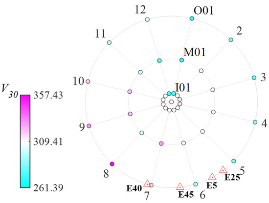
Figure 1.
Layout of the SMART 1 array and the azimuth directions of different events relative to the central station.
Four sets of reverse-mechanism waveforms recorded by the SMART 1 array were acquired from the PEER NGA-WEST2 database. Table 1 lists the metadata of the four events. is the Joyner–Boore distance to the rupture plane. Similar to previous studies [29,30], we used the data in the S-wave window, which is assumed to be stationary. Earthquake records were aligned before further processing. The aligning process considers both the time and frequency-domain features of the records, i.e., the autocorrelation peaks of the S-wave window data and the group delay of their Fourier spectra. The S-wave window lengths were determined based on both the time-domain features of the aligned records and the results from previous studies [29,31,32]. Periodograms cannot be affected by the alignment process. Therefore, the preprocessing does not affect the amplitude variation features of the periodogram.

Table 1.
Metadata of earthquakes.
In each of the four sets of ground motions, unavailable records exist. Illustrations in Figure 2 present five conditions of the unavailable records, including zero, one, two, and six records being unavailable. The unavailable records impose a nonnegligible influence on the estimation of the statistical value and will be introduced in the next section.
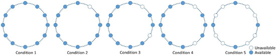
Figure 2.
Conditions of unavailable records in the SMART 1 record.
3. Comparison of the Statistical Features between the Gaussian Model and SMART 1 Records
In this section, existing approaches for describing the spatial variation of ground motions are briefly reviewed first. Then, a conditional method based on the Cholesky decomposition and the eigenvalue decomposition is developed to investigate the statistical features of the periodograms’ amplitude variation. Normalized periodogram loop variance (NPLV) is defined to measure the periodograms’ amplitude variation. The NPLV of the Gaussian model and the actual records are studied and compared.
3.1. Description of the Spatially Varying Ground Motions
The cross-PSD matrix describes the second-order statistical feature of a random field, with elements that can be expressed as follows.
where and are the cross-PSD function and the coherence function between the ground displacement and , respectively. The phase of is mainly composed of the wave-passage and site-response effect. In this study, the variation of the periodograms is of concern. Therefore, this study considers only the spectral coherence function’s amplitude. is the amplitude of the spectral coherence function. Two spectral coherence models are used, including the Harichandran–Vanmarcke model [33] (HV model), shown in Equation (2),
where and , and the Luco-Wong model [34] (LW model), shown in Equation (3).
The HV model with two parameter settings, denoted by HV1 and HV2, respectively, and the LW model with one parameter setting are chosen for studying the influence of coherence shape on the analysis results. The HV model is empirical. Table 2 lists the two-parameter settings, which Harichandran et al. [35] fitted with different earthquake records from the SMART 1 array. The LW model is semi-empirical. Zerva [36] recommended adopting a universal parameter of in this model. The three spectral coherence model for separation distance of 200m and 1km are demonstrated and compared in Figure 3.
Table 2.
Parameter settings for the HV spectral coherence model.
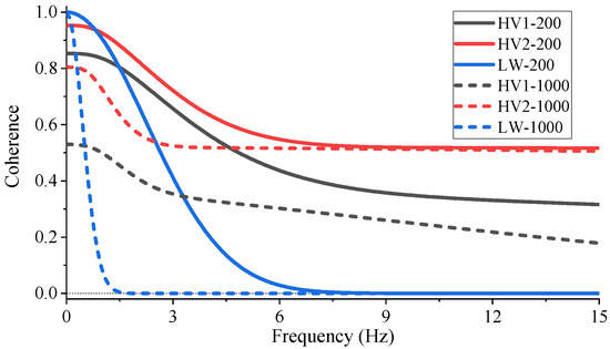
Figure 3.
Comparison of spectral coherence functions.
A ground-motion time series can be represented by the Fourier series expansion in Equation (4).
where and are the Fourier coefficients. When the ground motion belongs to a random field, the Fourier coefficients of the ground motions should satisfy Equations (5) and (6).
where and are independent, random Fourier coefficients exhibiting the zero-mean Gaussian distribution. To guarantee the Fourier coefficients satisfy Equations (5) and (6), some researchers apply Cholesky decomposition, while some apply eigenvalue decomposition. These methods assume that random components constitute a ground motion, as in Equation (7). The number counts in both the seed and the target ground motions.
where and are independent random variables exhibiting the standard normal distribution. The seed ground motion is also assumed to be realized by random variables. satisfies Equation (8).
The differences between the different conditional simulation methods are how to calculate , in other words, how to distribute the energy among the random variables.
3.2. Amplitude Variation of the Normalized Periodograms
In this study, for each earthquake event, the record from the central station is assumed to be the only seed ground motion. The other earthquake records are regarded to be conditionally generated from the seed ground motion. The Cholesky decomposition-based methods have one merit for theoretical analysis. When one seed is available, and the other locations are located the same distance from the location of the seed ground motion, the proportions of the seed ground motion in the conditional generated artificial ground motion are the same. Then, the eigenvalue decomposition-based method is used because the eigenvalue decomposition can result in symmetric coefficient matrices, while the results of the Cholesky decompositions cannot. The above process is introduced in detail as follows.
The cross-PSD matrix of a random field with uniform soil conditions can be expressed as Equation (9).
The diagonal elements of are all one, and the other elements are the spectral coherences. Conducting the Cholesky decomposition such that , Equation (10) presents the result of . Here, in matrix satisfies Equation (11)
Then, the eigenvalue decomposition to is conducted to distribute the remaining energy among the independent random variables. The coefficients can be calculated by Equation (12).
is an element of , and and are the eigenvector and eigenvalue matrix of , respectively. In Equation (12), the square root of a general matrix is defined as the matrix with eigenvalues that are the square root of , equal to the square root of the diagonal elements. Then, the Fourier coefficients of the conditional simulated ground motion at location can be represented as follows.
where is the row of matrix , and are random vectors with elements that exhibit the standard normal distribution. and are the Fourier coefficients of the seed ground motion.
After the previous decomposition approach, the periodogram of the conditional simulated ground motions can be expressed as Equation (14).
where represents the complex conjugate transpose of matrix , , , and . The expected value of is equal to Equation (15).
According to Rencher and Schaalje [37], for a quadratic form , the variance of can be obtained by Equation (16). The elements in the vector exhibit independent normal distributions.
Regarding the seed ground motion as a random process, the means of its Fourier coefficients are and , and the variances are 0. Then, the variance of the periodogram is derived as Equation (17).
To eliminate the influence of spectral shape, the ground motion periodograms are divided by the PSD of the random field. The result, i.e., , is called the normalized periodogram. When the statistical features of several earthquakes are concerned, the inter-event variance of at location is equal to Equation (18).
However, the SMART 1 array records in a particular earthquake are correlated. In this study, the quantity of events is far smaller than the number of records in a specific loop of an earthquake. Therefore, the intra-event loop variance of , instead of the inter-event variance in Equation (18), is adopted for studying the periodograms’ amplitude variation. The intra-event loop variance is a value estimated from the 12 stations in each loop and can be called the loop variance for brevity. A closed-form expression of the loop variance of is not available. In this study, the loop variances of were estimated by Monte Carlo simulating from 12 evenly separated stations, by considering the spectral coherence between stations. The results obtained from ten thousand simulations were used for evaluating each statistic. These results are presented in Figure 4b. The theoretical inter-event variances of in Equation (18) are plotted in Figure 4a for comparison. Figure 4a uses abbreviations to represent the results calculated by the different spectral models with varying separation distances. For example, HV1-200 means the results yielded by the HV1 model, and the parameter of separation distance is 200 m. When the spectral coherences between the loop stations are zero, the theoretical inter-event loop variance of in Equation (18) equals the loop variance of . However, the spectral coherences between the loop stations and the central station are not zero. Comparing Figure 4a with Figure 4b, the loop variances of are obviously more minor than its inter-event variances. Therefore, spectral coherence should be considered when analyzing the spectral amplitude variation. Comparing the results calculated by the HV1 model and the LW model, the significant differences also indicate that the spectral coherence’s shape dramatically influences the shape of the loop variance.
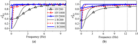
Figure 4.
Variances of calculated using HV and LW spectral coherence models: (a) inter-event variance of and (b) loop variance of .
Regarding actual ground motions, the PSD of the concerning random field is not accessible. Therefore, the square of the coefficient of variance (SCV) is adopted to estimate the loop variance of the normalized periodogram. Researchers have developed the distribution of the coefficient of variance of normally distributed random variables [38] and lognormal distribution random variables [39]. However, the statistical features of the coefficient of variance for the quadratic form of normal distribution remain unknown. Consequently, Monte Carlo simulations were carried out to investigate the relationship between the loop variances and the SCV. Figure 5 shows the comparison of the loop variance with the loop SCV. Both the results calculated from the HV1 and the LW models show a significant difference between the loop variance and loop SCV. The differences are frequency-dependent and, thus, cannot be replaced by a constant value. Using the loop SCV calculated with a small amount of data for approximating the loop variance can result in significant deviations.
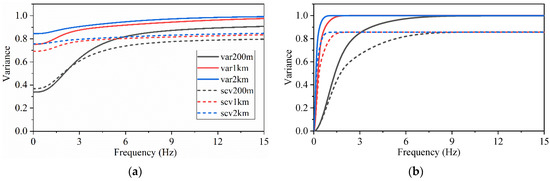
Figure 5.
Loop variance vs. loop SCV: (a) HV1 model and (b) LW model.
An adjustment coefficient, denoted by , is introduced to restore the loop SCV to the loop variance.
where represents the loop variance estimated from the simulations corresponding to 12 evenly distributed stations, means the loop SCV is calculated with the simulations corresponding to stations. As stated in Section 2, the data obtained from the PEER center consist of unavailable records. The influence of unavailable records on the adjustment coefficient is also investigated by conducting Monte Carlo simulations. Figure 6 shows the adjustment coefficients for different unavailable record conditions. As shown in this figure, the more records that are unavailable, the more significant the adjustment coefficients are.
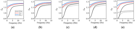
Figure 6.
Adjustment coefficient for different loop configurations: (a) condition 1, (b) condition 2, (c) condition 3, (d) condition 4, and (e) condition 5.
Then, the estimated loop variances of the records’ normalized periodograms for different events and their components in different directions are shown in Figure 7. The normalized periodogram loop variances (NPLVs) are calculated by first calculating the SCV of the corresponding loop. Next, the resulting SCVs are multiplied by the adjustment coefficient according to the unavailable record conditions. The NPLVs of the records are denoted by , and for the inner, middle, and outer loops, respectively. The inter-event mean value of the NPLVs, which is the averaged NPLVs of all the horizontal components of the different events, is presented with bold red lines in each subgraph.
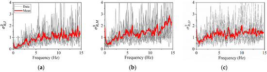
Figure 7.
Loop variance of in different loops: (a) inner loop, (b) middle loop, and (c) outer loop.
In each subgraph of Figure 7, the NPLVs show features similar to that of the FAS amplitude variation reported by Liao and Zerva [14]. As shown in this figure, the NPLVs increase with frequency and reach a relatively steady stage at 6.25 Hz, which is 1/16 of the sampling frequency. In Figure 7b, the average NPLV beyond 12.5 Hz continues to increase to an extremely high value, which can be attributed to the dividing of the small value when calculating the SCV of the normalized periodograms. The energy in the PSD of the five events beyond 12.5 Hz is small and has a low signal-to-noise ratio. The NPLVs for different loops in different events exhibit similar trends with the increase in frequency, indicating that the NPLV is a suitable index for describing spectral amplitude variation. The average of the inter-event mean value of the NPLVs between 6.75 and 12.25 Hz for each loop, denoted by , , and , respectively, are listed in Table 3.
Table 3.
Averaged NPLVs for different loops.
As shown in the previous section, based on the assumption of the Gaussian model, the value of an NPLV should be less than 1. Consequently, the analysis above shows that the Gaussian model underestimates the periodograms’ amplitude variation of the actual ground motions.
3.3. Power Variation of SMART 1 Records
In this subsection, the ground motion power variation of the SMART 1 array records is analyzed to show, in another aspect, that the Gaussian model results in an underestimation of spectral amplitude variation.
First, the power variation with the variation of separation distance is investigated. The ground motion power is the integral of the periodogram in the frequency domain. For loop , ’s mean and standard deviation are represented by and , respectively. The superscript can be replaced by , , and . The power ratio is defined by the ground motion power divided by the power of the central station periodogram, i.e., . The mean power ratios in loop of event , represented by , are plotted by the bold lines with symbols in Figure 8a. The average of all the horizontal components of different events in loop is denoted by . The results of are plotted with fine horizontal lines in this figure. The for the inner, middle, and outer loops are all approximately 90%, indicating that the averaged power changes slightly with the increase in the loop radius. The power of the central station records is greater than that of all the other loops, which systematic reasons outside the scope of this study might cause, such as complex soil-layer distributions and path effects. However, the power of the central-station records remains within one standard deviation from the average power of the other loops. Thus, this difference might also be attributed to the small sample size.
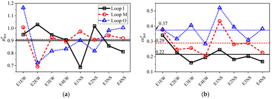
Figure 8.
Power conditions for different events: (a) power ratio and (b) normalized power loop standard deviation.
Next, the loop power variation is used to describe the power variation of the SMART 1 random field. To compare the loop power variation among different events, the normalized power loop standard deviation is defined as . is calculated for the horizontal components of different events and is plotted with bold lines in Figure 8b. The average of all the events and directions is plotted with fine lines and marked with the average values. In this figure, the difference between events are sometimes smaller than the difference between different components in the same event. Therefore, the inter-event power variation is assumed to be negligible. In general, increases with the loop radius.
Monte Carlo simulations were carried out with the conventional Gaussian model. Each estimation adopted ten thousand simulation results. The central station records were used as seeds, and the averaged periodograms of actual earthquakes in each loop were used as the PSD to generate artificial periodograms at different stations. Define the normalized power loop standard deviation, denoted by , as Equation (20). is the counterpart of for the simulated periodograms. Figure 9 presents the results of . is the power of the central station record.
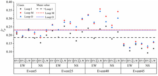
Figure 9.
Simulated normalized power loop standard deviation with Gaussian model.
As shown in this figure, the spectral coherence model can cause a significant difference between the simulated value. Its influence can be more significant than the influence of separation distance but far smaller than the influence of the target PSD of the random field. When the conventional Gaussian model is used, the maximum is 0.37, and the average of all the components is 0.230 for the outer loop. These values are all far smaller than the actual ground motions. The above analysis shows that the conventional Gaussian model underestimates the power loop variation. This conclusion is a side-proof of the study about the periodograms’ amplitude variability in previous sections.
4. Modification of the Gaussian Model
In this section, a modification is made to the Gaussian model to realize the periodograms’ amplitude variation features of the SMART 1 records shown in Figure 7. The statistical characteristics of the modified model and its parameters are investigated.
The modified Gaussian model is acquired by multiplying Equation (14) by a local power variation coefficient , as shown in Equation (21). The modified Gaussian model retains the main structure of the conventional Gaussian model. is a random variable with a mean value of one and a variance of .
In Equation (21), is a coefficient that serves as an amplifier of the periodogram. Since the expected value of is one, it neither affects the target spectrum nor the spectral coherence relationship between any two realized periodograms. Moreover, should be greater than zero.
at different locations are correlated, making the properties of similar to the periodograms at a particular frequency. On account of the previous requirements, assume is exhibiting a noncentral Wishart distribution [40]. The simulated at location can be generated by a Gaussian quadratic form, as shown by Equation (22).
where is the row of matrix , can be solved by any conditional simulating methods, such as Cholesky decomposition. Defining as the cross-variance matrix of , then satisfies . is a vector of random variables with elements that are independent and exhibit the standard normal distribution. The local power coefficient of the seed ground motion is assumed to be 1. is the number of quadratic forms in the summation of Equation (22). The larger is, the smaller the kurtosis of is. When approaches infinity, approaches a normal distribution. When the spectral coherence among locations approaches zero, approaches a chi-squared distribution, i.e., . The variance and kurtosis of are and , respectively.
should be a proper value that is not too large in case the variance of is not large enough to capture the expected NPLV nor too small in case the fourth moment of the periodogram become too large to have a stable estimation of the second moment with a small sample size.
Regarding artificial ground motion simulation, the Fourier coefficients simulated by the conventional Gaussian model are multiplied by the square root of . Equation (23) shows the formula of ground motions simulated by the modified Gaussian model.
where and are the Fourier coefficients generated by the conventional Gaussian-model-based conditional methods, can be directly calculated by .
Figure 10 shows the realization of the normalized periodograms’ variance and coefficient of variance when equal to 12. The subscript and represent the results realized by the conventional Gaussian model and the modified model, respectively. As shown in this figure, the SCVs are smaller than the variances of the periodograms, which is consistent with the conclusion derived in the previous section. The SCV realized by the Gaussian model is smaller than one and obviously smaller than the actual ground motion.
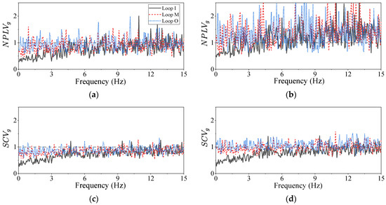
Figure 10.
Numerical realization of the normalized periodograms’ variance and SCV: (a) variance of Gaussian model, (b) variance of modified Gaussian model, (c) SCV of Gaussian model, and (d) SCV of modified Gaussian model.
The variance and coherence between at different locations cannot be solved directly. In this study, a genetic algorithm is used to search for the coherence of , such that the simulated NPLVs comply with the actual ground motions in Table 3. Monte Carlo simulations were carried out to calculate the NPLVs with the modified Gaussian model.
In the SMART 1 array, 37 stations possess 36 unique separation distances. The coherence value for these separations should be updated, which should be smaller than one and greater than zero. The derivative of a coherence model with respect to separation distance should be smaller than zero because the coherence is expected to decrease with the increase in separation distance. Therefore, the coherence of , denoted by , is assumed to possess a form as shown by Equation (24).
where is the distance between two locations, and is the function’s parameter to be fitted. Since , and is expected to decrease with the increase in , thus, the following equations should be established.
In the Monte Carlo simulations, when , was forced to be zero, and when , was forced to be one. The NPLVs of the modified Gaussian model are estimated with ten thousand simulation results. The difference between the simulated NPLVs and the actual ground motions is defined as Equation (26).
where represents the Euclidean norm of the inner variable . The conditions when and are studied to show the influence of on the coherence of .
Table 4 lists the fitted results of the parameters in Equation (24). The fitness results when are better than when .
Table 4.
Results of the searched parameters and fitness values.
Table 5 lists the results of the averaged NPLVs and their error ratios relative to the actual records for different . The averaged NPLVs of actual earthquakes can be referred to in Table 3. As detailed in Table 5, nearly all the results from the model when are better than those when . Figure 11 demonstrates the fitted results of coherence model for different and different spectral coherence models. As shown in Figure 11b, all the fitted coherence models of reach zero far before the separation distance reaches four kilometers. At this condition, has reached its greatest possible variance. Still, this value is insufficient to realize the NPLVs of actual earthquake records.
Table 5.
Simulated averaged NPLVs for different spectral coherence models and different .
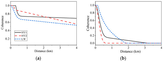
Figure 11.
Coherence of estimated by different spectral coherence models : (a) and (b) .
The search result when is shown in Figure 11a. None of the fitted coherence reaches zero. For this condition, the fitting accuracy depends mainly on the functional form chosen in Equation (24).
The characteristics of the fitted coherence in Figure 11a estimated from different spectra show no features in common, indicating that the coherence of should be calculated according to the spectral coherence model.
Figure 12 shows the NPLVs realized by different spectral coherence models. As shown in Figure 12, the results obtained by the modified Gaussian model amplify the NPLV compared with those obtained by the Gaussian model.
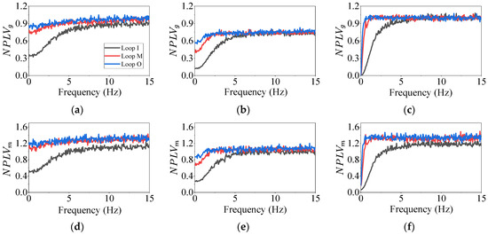
Figure 12.
Influence of spectral coherence models (a) HV1, (b) HV2, (c) LW, (d) HV1, (e) HV2, and (f) LW on the NPLVs calculated by (a–c) Gaussian model and (d–f) modified Gaussian model.
In this study, is assumed to be a frequency-independent random variable. However, the spectral coherence model has a significant influence on the shape of NPLVs between 0 and 5 Hz. Further studies should be carried out to reveal the dependency of on the frequency.
5. Conclusions
In this study, by examining the compliance of the conditional simulated random field by the Gaussian model with the spectral features of four groups of SMART 1 array earthquake records, the conventional Gaussian model was confirmed to underestimate the periodograms’ amplitude variation of the actual ground motions. A modified Gaussian model is developed to tackle the detected defects. An LPC was introduced as an amplifier of the periodogram. The LPC is a random variable exhibiting a noncentral Wishart distribution; the mean value of the LPC is one, and the variance increases with the separation distance. A simulation method for the LPC based on the conventional CPDF method was developed. Monte Carlo simulations and the genetic algorithm method were combined to search the coherence model of the LPC. The LPC’s coherence models for three different spectral coherence models are calculated. The results of the Monte Carlo simulations show that the modified Gaussian model is more effective in describing the periodograms’ amplitude variation than the conventional Gaussian model. The following conclusions were summarized.
- The periodogram’s loop SCV underestimates the periodogram’s loop variance when the spectral coherence is small.
- The conventional Gaussian model underestimates the power loop variance and the periodogram’s loop variance of the actual earthquake records.
- The spectral coherence model has a significant influence on the coherence of the LPC. The fitted LPC’s coherence model depends highly on the chosen spectral coherence model. As a result, no general LPC coherence model can be obtained.
Author Contributions
Conceptualization, H.Q. and L.L.; Methodology, H.Q.; Software, H.Q.; Validation, H.Q.; Formal analysis, H.Q.; Data curation, H.Q.; Writing—original draft, H.Q.; Writing—review & editing, H.Q. and L.L.; Supervision, L.L.; Project administration, L.L.; Funding acquisition, L.L. All authors have read and agreed to the published version of the manuscript.
Funding
This work and APC was supported by the National Natural Science Foundation of China, Grant No. 51678116.
Data Availability Statement
The earthquake waveform and the corresponding metadata were acquired from the Pacific Earthquake Engineering Research Center (PEER). https://ngawest2.berkeley.edu/site, accessed on 22 November 2022.
Acknowledgments
The earthquake waveform and the corresponding metadata were acquired from the Pacific Earthquake Engineering Research Center.
Conflicts of Interest
The authors declare no conflict of interest.
References
- Somaini, D.R. Seismic behaviour of girder bridges for horizontally propagating waves. Earthq. Eng. Struct. Dyn. 1987, 15, 777–793. [Google Scholar] [CrossRef]
- Soyluk, K.; Dumanoglu, A.A. Comparison of asynchronous and stochastic dynamic responses of a cable-stayed bridge. Eng. Struct. 2000, 22, 435–445. [Google Scholar] [CrossRef]
- Allam, S.M.; Datta, T. Seismic response of a cable-stayed bridge deck under multi-component nonstationary random ground motion. Earthq. Eng. Struct. Dyn. 2004, 33, 375–393. [Google Scholar] [CrossRef]
- Sextos, A.; Karakostas, C.; Lekidis, V.; Papadopoulos, S. Multiple support seismic excitation of the Evripos bridge based on free-field and on-structure recordings. Struct. Infrastruct. Eng. 2015, 11, 1510–1523. [Google Scholar] [CrossRef]
- Loh, C.; Penzien, J.; Tsai, Y. Engineering analyses of SMART 1 array accelerograms. Earthq. Eng. Struct. Dyn. 1982, 10, 575–591. [Google Scholar] [CrossRef]
- Katayama, T.; Yamazaki, F.; Nagata, S.; Lu, L.; Turker, T. A strong motion database for the Chiba seismometer array and its engineering analysis. Earthq. Eng. Struct. Dyn. 1990, 19, 1089–1106. [Google Scholar] [CrossRef]
- Svay, A.; Perron, V.; Imtiaz, A.; Zentner, I.; Cottereau, R.; Clouteau1, D.; Bard, P.Y.; Hollender, F.; Lopez-Caballero, F. Spatial coherency analysis of seismic ground motions from a rock site dense array implemented during the Kefalonia 2014 aftershock sequence. Earthq. Eng. Struct. Dyn. 2017, 46, 1895–1917. [Google Scholar]
- Goulet, C.A.; Kottke, A.; Boore, D.M.; Bozorgnia, Y.; Hollenback, J.; Kishida, T.; Der Kiureghian, A.; Ktenidou, O.J.; Kuehn, N.M.; Rathje, E.M.; et al. Effective amplitude spectrum (EAS) as a metric for ground motion modeling using Fourier amplitudes. In Proceedings of the 2018 Seismology of the Americas Meeting, Miami, FL, USA, 17 May 2018. [Google Scholar]
- Bayless, J.; Abrahamson, N.A. Summary of the BA18 ground-motion model for Fourier amplitude spectra for crustal earthquakes in California. Bull. Seismol. Soc. Am. 2019, 109, 2088–2105. [Google Scholar] [CrossRef]
- Bayless, J.; Abrahamson, N. An Empirical Model for Fourier Amplitude Spectra Using the NGA-West2 Database; PEER 2018/07; Pacific Earthquake Engineering Research Center, Headquarters at the University of California: Berkeley, CA, USA, 2018; Available online: https://peer.berkeley.edu/news/new-peer-report-201807-empirical-model-fourier-amplitude-spectra-using-nga-west2-database (accessed on 21 October 2022).
- Abrahamson, N. Spatial Variation of Earthquake Ground Motion for Application to Soil-Structure Interaction; Electric Power Research Institution: Palo Alto, CA, USA, 1992. [Google Scholar]
- Ancheta, T.D.; Stewart, J.P.; Abrahamson, N.A. Engineering characterization of earthquake ground motion coherency and amplitude variablity. In Proceedings of the IAEE International Symposium: Effects of Surface Geology on Seismic Motion 2011, Santa Barbara, CA, USA, 23–26 August 2011; Santa Barbara: Los Angeles, CA, USA, 2011. [Google Scholar]
- Abrahamson, N. Generation of spatially incoherent strong motion time histories. In Proceedings of the Earthquake Engineering, Tenth World Conference, Madrid, Spain, 19−24 July 1992; Balkema: Rotterdam, The Netherlands, 1992. [Google Scholar]
- Liao, S.; Zerva, A. Physically compliant, conditionally simulated spatially variable seismic ground motions for performance-based design. Earthq. Eng. Struct. Dyn. 2006, 35, 891–919. [Google Scholar] [CrossRef]
- Kameda, H.; Morikawa, H. An interpolating stochastic process for simulation of conditional random fields. Probabilistic Eng. Mech. 1992, 7, 243–254. [Google Scholar] [CrossRef]
- Rodda, G.K.; Basu, D. Spatial variation and conditional simulation of seismic ground motion. Bull. Earthq. Eng. 2018, 16, 4399–4426. [Google Scholar] [CrossRef]
- Abrahamson, N. Spatial interpolation of array ground motions for engineering analysis. In Proceedings of the Ninth World Conference on Earthquake Engineering, Tokyo, Japan, 4 December 1988. [Google Scholar]
- Zerva, A. Seismic ground motion simulations from a class of spatial variability models. Earthq. Eng. Struct. Dyn. 1992, 21, 351–361. [Google Scholar] [CrossRef]
- Ramadan, O.; Novak, M. Simulation of spatially incoherent random ground motions. J. Eng. Mech. 1993, 119, 997–1016. [Google Scholar] [CrossRef]
- Vanmarcke, E.H.; Fenton, G.A. Conditioned simulation of local fields of earthquake ground motion. Struct. Saf. 1991, 10, 247–264. [Google Scholar] [CrossRef]
- Krige, D. Two-dimensional weighted moving average trend surfaces for ore-evaluation. J. S. Afr. Inst. Min. Metall. 1966, 66, 13–38. [Google Scholar]
- Vanmarcke, E.H.; Heredia-Zavoni, E.; Fenton, G.A. Conditional simulation of spatially correlated earthquake ground motion. J. Eng. Mech. 1993, 119, 2333–2352. [Google Scholar] [CrossRef]
- Shinozuka, M.; Zhang, R. Equivalence between Kriging and CPDF methods for conditional simulation. J. Eng. Mech. 1996, 122, 530–538. [Google Scholar] [CrossRef]
- Morikawa, H.; Kameda, H. Conditional random fields containing nonstationary stochastic processes. Probabilistic Eng. Mech. 2001, 16, 341–347. [Google Scholar] [CrossRef]
- Wang, L. Stochastic Modeling and Simulation of Transient Events; University of Notre Dame: Notre Dame, IN, USA, 2008. [Google Scholar]
- Hu, L.; Xu, Y.L.; Zheng, Y. Conditional simulation of spatially variable seismic ground motions based on evolutionary spectra. Earthq. Eng. Struct. Dyn. 2012, 41, 2125–2139. [Google Scholar] [CrossRef]
- CEN. Eurocode 8: Design of Structures for Earthquake Resistance-Part 1: General Rules, Seismic Actions and Rules for Buildings; European Committee for Standardization: Brussels, Belgium, 2005. [Google Scholar]
- Abrahamson, N.A.; Bolt, B.A.; Darragh, R.B.; Penzien, J.; Tsai, Y.B. The SMART I accelerograph array (1980–1987): A review. Earthq. Spectra 1987, 3, 263–287. [Google Scholar] [CrossRef]
- Zerva, A.; Zervas, V. Spatial variation of seismic ground motions: An overview. Recent Dev. World Seismol. 2002, 55, 271–297. [Google Scholar] [CrossRef]
- Abrahamson, N. Spatial Coherency Models for Soil-Structure Interaction; Draft EPRI Report; Electric Power Research Institute: Palo Alto, CA, USA, 2005. [Google Scholar]
- Hao, H.; Oliveira, C.; Penzien, J. Multiple-station ground motion processing and simulation based on SMART-1 array data. Nucl. Eng. Des. 1989, 111, 293–310. [Google Scholar] [CrossRef]
- Loh, C.H. Analysis of the spatial variation of seismic waves and ground movements from smart-1 array data. Earthq. Eng. Struct. Dyn. 1985, 13, 561–581. [Google Scholar] [CrossRef]
- Harichandran, R.S.; Vanmarcke, E.H. Stochastic variation of earthquake ground motion in space and time. J. Eng. Mech. 1986, 112, 154–174. [Google Scholar] [CrossRef]
- Luco, J.; Wong, H. Response of a rigid foundation to a spatially random ground motion. Earthq. Eng. Struct. Dyn. 1986, 14, 891–908. [Google Scholar] [CrossRef]
- Harichandran, R.S.; Hawwari, A.; Sweidan, B.N. Response of long-span bridges to spatially varying ground motion. J. Struct. Eng. 1996, 122, 476–484. [Google Scholar] [CrossRef]
- Zerva, A. Spatial Variation of Seismic Ground Motions: Modeling and Engineering Applications; CRC Press: Boca Raton, FL, USA, 2016. [Google Scholar]
- Rencher, A.C.; Schaalje, G.B. Linear Models in Statistics; John Wiley & Sons: Hoboken, NJ, USA, 2008. [Google Scholar]
- Sokal, R.R.; Rohlf, F.J. Biostatistics; Francise & Co.: New York, NY, USA, 1987. [Google Scholar]
- Koopmans, L.H.; Owen, D.B.; Rosenblatt, J.I. Confidence intervals for the coefficient of variation for the normal and log normal distributions. Biometrika 1964, 51, 25–32. [Google Scholar] [CrossRef]
- Mathai, A.M.; Provost, S.B. Quadratic Forms in Random Variables: Theory and Applications; Marcel Dekker: New York, NY, USA, 1992. [Google Scholar]
Publisher’s Note: MDPI stays neutral with regard to jurisdictional claims in published maps and institutional affiliations. |
© 2022 by the authors. Licensee MDPI, Basel, Switzerland. This article is an open access article distributed under the terms and conditions of the Creative Commons Attribution (CC BY) license (https://creativecommons.org/licenses/by/4.0/).