Article

Soft Computing Approach to Design a Triple-Band Slotted Microstrip Patch Antenna

by
Mahmud Esad Yiğit
1,2,*,
Gülay Öke Günel
3,
Mustafa Emre Aydemir
4 and
Tayfun Günel
5
1
Department of Electrical and Electronics Engineering, Çankırı Karatekin University, Çankırı 18100, Turkey
2
Graduate School, Department of Electronics & Communication Engineering, Istanbul Technical University, Istanbul 34469, Turkey
3
Control and Automation Engineering Department, Istanbul Technical University, Istanbul 34469, Turkey
4
Department of Electrical and Electronics Engineering, Istanbul Esenyurt University, Istanbul 34510, Turkey
5
Department of Electronics & Communication Engineering, Istanbul Technical University, Istanbul 34469, Turkey
*
Author to whom correspondence should be addressed.
Appl. Sci. 2022, 12(23), 11923; https://doi.org/10.3390/app122311923
Submission received: 10 October 2022 / Revised: 12 November 2022 / Accepted: 14 November 2022 / Published: 22 November 2022
(This article belongs to the Section Electrical, Electronics and Communications Engineering)

Abstract

:
The design process of antenna structures that meet up-to-date requirements takes a long time and brings a high computational load. In this paper, an approach based on Soft Computing (SC) techniques was used to shorten the design time and to achieve an antenna structure that yields performance characteristics as close as possible to the desired values. In order to obtain a microstrip patch antenna with the targeted characteristics and the best accuracy in a faster way, a Support Vector Machine (SVM)-based regression model was employed. A triple-band microstrip antenna with desired resonance frequencies and gain values was designed by using the Support Vector Regression (SVR) model by introducing multiple slots and arc-truncation to the patch antenna. Simulation results of the High-Frequency Structural Simulator (HFSS) and measurements of implementation of the designed antenna are given. Performance characteristics of the obtained antenna are also compared with those given in the literature, which have triple-band properties. In addition, the antenna was redesigned using the optimization tool in HFSS for comparison. The accuracy of the results and required time for design were compared for both the SVR model approach and the HFSS optimization tool.

1. Introduction

Soft computing (SC) refers to a group of methods that achieve tractable, robust, and low-cost solutions for problems that involve imprecise and uncertain conditions. Soft computing techniques are mainly inspired by intelligence in nature, such as the functioning principles of the biological brain, the reasoning mechanism of the human mind, or the natural selection principles of evolutionary processes. The term “Soft Computing” was proposed by Lotfi A. Zadeh [1,2].
The results obtained in SC techniques are not mathematically exact; approximate optimum results are obtained, whereas, in Hard Computing (HC), certain and precise results are attained. However, this increases computational time and load. In addition, HC requires the ideal model of the system or analytical expressions describing the behavior of the system and is not suitable for complex real-world problems where ideal model is not available. SC is the aggregation of various computational techniques. Some of the SC techniques and their applications include fuzzy logic [1,2], evolutionary algorithms [3,4,5,6,7,8,9,10,11,12,13,14,15,16,17,18], artificial neural networks (ANN) [19,20,21,22,23,24,25,26,27], and support vector machines (SVM) [19,20,28].
SVMs have been introduced by Vapnik [19,28]. Briefly, SVMs set up a hyperplane that separates two different sample sets from each other with a maximum margin in classification [20]. SVMs have usually been used for classification, but they are also used in regression problems and are named Support Vector Regressors (SVR). SVRs have proven their capabilities in various studies of electromagnetics and microwaves due to their generalization properties [29,30,31,32,33,34,35,36]. They are used to design single-band antennas [32,33,34,35,36].
Electromagnetic simulation programs are used for antenna analysis and synthesis [37,38,39]. As the number of design parameters increases, the processing load and the time spent in the analyses performed by these programs also increase. Antennas need to be optimized with the changes in geometric structure to obtain the desired response. This also increases the design time. Even if the designer’s knowledge and experience are sufficient, repetitively running programs with/without optimization or trial and error method negatively affects the design time. Furthermore, successful results are not guaranteed after repetitive trials.
Nowadays, there are many studies on the analysis and synthesis of microstrip antennas. Microstrip antennas have gained great interest since they were first introduced due to their features such as easy fabrication, low cost, compatibility with integrated circuits, and low weight. Moreover, by adding slots on the microstrip antenna patch and/or ground, antenna performance can be improved easily and efficiently. However, a general analytical formula for slots with various numbers and different types are not given in the literature so far. Additionally, the complexity of the design and time spent are increased with the number of slots.
In this paper, in order to overcome these drawbacks, a soft computing-based method is utilized in the design of a microstrip patch antenna that operates in triple-band. The resonance frequency and gain that yield the desired performance are obtained by utilizing an SVR model. Multiple slots and arc truncation [40,41] are implemented to patch the antenna to obtain an antenna that operates in triple-band with desired gains. The desired resonance frequencies of the triple-band are selected in 2.4 and 5 GHz bands of Wireless Local Area Network (WLAN) and the n80 (4.4–4.9 GHz) band [42] of 5G. There are two main novelties of the work presented, the first one is the novel structure of a triple-band antenna, and the second novelty is the implementation of a triple-band antenna designed using SVR for the first time. As far as the authors know, this work presents the first implementation of a triple-band antenna designed via SVR.
In order to verify the performance of the proposed antenna design method, simulation and implementation results are presented. Additionally, the achieved performance is compared with those of several antenna designs in the literature. The obtained results demonstrate the superiority of the proposed approach.
The contents of this paper are as follows: After this brief introduction, Section 2 presents a brief overview of Support Vector Regression. Section 3 describes the proposed design method for the triple-band antenna. Simulation and implementation results, as well as a comparison with existing designs in the technical literature, are presented in Section 4. Additionally, a comparison with the design carried out with the HFSS optimization tool is provided in Section 5. Section 6 briefly concludes the paper.

2. Theory of Support Vector Regression

A training data set S can be given by
S = { x i ,   y i } i = 1 N x i X n ,   y
where N is the number of elements in S and n is the dimension of the input. S can be represented by the regression model [20]:
y i = w , Φ ( x i ) + b         i = 1 , 2 , . N
where Φ ( x i ) is the image of the input data in feature space, b is regressor bias, and w is a weighting vector. The aim of the optimization is to find the optimal regressor within ε tube by minimizing the training error and optimizing the geometric margin. The primal form of the optimization problem can be formulated as [20,43,44]:
min ( w , b ) 1 2 w 2 + C i = 1 N ( ξ i + ξ i * )
subject to
y i w , Φ ( x i ) b ε + ξ i w , Φ ( x i ) + b y i ε + ξ i *   ξ i ,     ξ i * 0 ;           i = 1 ,   2 ,   ,   N
where ε is the upper limit for the acceptable error, the slack variables ξ i and ξ i * define the deviation from the ε tube [43,44]. The constraints of the optimization problem are constructed by an ε insensitive loss function [44,45]. The primal function and its constraints are used to define a Lagrange function. Lagrangian can be derived by combining the primal function and related constraints by presenting non-negative Lagrange multipliers β, β *, η, and η * [43,44]:
L = 1 2 w 2 + C i = 1 N ( ξ i + ξ i * ) i = 1 N β i ( ε + ξ i y i + w , Φ ( x i ) + b ) i = 1 N β i * ( ε + ξ i * + y i w , Φ ( x i ) b ) i = 1 N ( η i ξ i + η i * ξ i * )
Here, C is a parameter that controls the trade-off between the complexity of the obtained model and the number of non-separable points. For optimality, the partial derivatives of the Lagrangian with respect to primal variables have to vanish because of the saddle point property of the Lagrangian with respect to the primal variables and dual variables at the solution [44]:
L w = 0     w i = 1 N β i w , Φ ( x i ) = 0
L b = 0     i = 1 N ( β i β i * ) = 0
L ξ i = 0     C β i η i = 0 ,     i = 1 , 2 , N
L ξ i * = 0     C β i * η i * = 0 ,     i = 1 , 2 , N
The dual form can be defined by using optimality conditions (6–9) in (5):
D = 1 2 i = 1 N j = 1 N ( β i β i * ) ( β j β j * ) K i j + ε i = 1 N ( β i + β i * ) y i i = 1 N ( β i β i * )
subject to
0 β i C 0 β i * C i = 1 N ( β i β i * ) = 0 i = 1 , 2 , N
where K i j is the kernel function and can be given by K i j = Φ T ( x i ) Φ ( x i ) . The dual form has a convex objective function with linear constraints; therefore, a global solution to the problem is guaranteed. The optimal solution to the dual problem can be achieved by employing a quadratic programming solver, and the Lagrange multipliers are obtained.
The training data with non-zero Lagrange multipliers constitute the “support vectors” [43,45,46]. The regression problem of (2) can be solved by estimation via the support vectors and the corresponding Lagrange multipliers:
y ^ ( x ) = i = 1 N λ i K ( x ,   x i ) + b ,       λ i = β i β i *
Mostly used kernel functions are linear, polynomial, and radial basis kernel (RBF) functions. RBF function can be given as:
K ( X i , X j ) = e x p ( γ X i X j 2 )
where γ is the Gaussian parameter and X is the training vector.
Wavelet functions can also be used as kernel functions [47,48,49,50] in SVR, as well as the functions mentioned above. Wavelet analysis has the advantage that it processes signals in both time and frequency domains. The prediction is achieved more accurately via wavelet kernel than other types of kernel functions [35]. The orthonormality of wavelet functions results in an increase in the generalization capability of SVR [47]. A wavelet function is defined as [47]
h a , b ( x ) = 1 a h ( x b a )
where a is the scaling factor and b is the shifting parameter. Wavelet kernel is derived as [47]
K ( X , X ) = i = 1 N h ( x i b i a ) h ( x i b i a )
where X and X are N-dimensional vectors, h(x) is a wavelet function and a ,   b i ,   b i ,   x i ,   x i R and X , X R N . Wavelet kernel independent of shifting is given as [47]:
K ( X , X ) = i = 1 N h ( x i x i a )
The Morlet wavelet function is defined as [47,48]:
h ( x ) = cos ( 1 . 75 x ) exp ( x 2 2 )
The Morlet wavelet kernel function is given as [47,48]:
K ( X , X ) = i = 1 N cos ( 1.75 ( x i x i ) a ) · exp ( x i x i 2 a 2 )
The Mexican-hat wavelet kernel function is written as [47,48]:
K K ( X , X ) = i = 1 N cos ( 1 ( x i x i ) 2 a ) · exp ( x i x i 2 2 a 2 )
In this study, wavelet kernel functions are preferred in the SVR approach due to their advantages, and specifically Mexican-hat wavelet kernel function is used since it has achieved the best results in the simulations. Other details related to the SVR design of the antenna are presented in the following sections.

3. Design of Triple-Band Antenna

Firstly, a rectangular microstrip patch antenna operating in 2.4 GHz of WLAN was designed by using formulations given in the literature [51].
The patch width (W) is computed by (20) for a rectangular microstrip patch antenna whose resonance frequency and relative permittivity of the substrate are f r and ε r , respectively [51]:
W = c 2 f r 2 ε r + 1
where c denotes the velocity of light in free space. The length of the antenna patch (L) can be calculated by [51]:
L = [ c 2 f r ε r e f f ] 2 Δ L
Here, ΔL is the extension of the length due to the effect of fringing fields and is given as [51]:
Δ L = 0.412 h ( ε r e f f + 0.3 ) ( W h + 0.264 ) ( ε r e f f 0.258 ) ( W h + 0.8 )
Effective permittivity ε r e f f is given by [51]:
ε r e f f = [ ε r + 1 2 ] + [ ε r 1 2 ] [ 1 + 12 h W ] 1 / 2
The desired resonance frequency of the rectangular microstrip patch antenna is selected as 2.4 GHz, WLAN base frequency. The antenna substrate is selected as Rogers RT/duroid 5870 with relative permittivity of 2.33, thickness of 0.787 mm, and loss tangent of 0.0012. By using (20–23), antenna patch dimensions L and W are computed as 38.6 mm and 47.5 mm, respectively. Then, parametric analysis in a High-Frequency Structural Simulator (HFSS) [37] is carried out to find the best reflection coefficient and input impedance and tune the resonance frequency to be close to 2.4 GHz for obtaining the feed location of the microstrip patch antenna without slots.
A parametric analysis method is used to simulate multiple variations for a design model [37]. A parametric analysis begins with the description of a series of variable values (variations) with chosen step sizes within a range. HFSS carries out an analysis of the design for each variation. Then, the results can be compared to see how each variation affects the performance of the design. Parametric analysis is frequently employed before the optimization process since it provides a reasonable range of variable values [37].
As a result of this process, the feed location of the antenna is computed as xf = 7.0 mm and yf = 0 mm. The same location is preserved for the microstrip patch antenna with triple slots and arc truncation.
After that, multiple slots were added to the conventional microstrip antenna that had the same patch dimensions and substrate to obtain multiband property. Then, the arc-truncation technique [40,41,52,53] was applied to the four edges of the antenna to improve gain performance. It is shown that there is an inverse relationship between the length of truncation and the Q factor of a truncated microstrip patch antenna [52,53]. Low radiation Q factor causes high antenna efficiency [52] value, which means high gain. In this study, it has also been observed that the reflection coefficient value decreases by introducing arc truncations to the antenna. This leads to an increase in the realized gain. The effect of the arc-truncation on the gain performance is ~1 dB increase. Center points for the two large slots are selected such that the slots are far away from the feed point and not so near to the edge of the antenna patch. The center point for the small slot is located at the upper half of the antenna patch. Thus, it is ensured that slots would not coincide with each other, feed point, and edges of the antenna. The initial positions of the slots were selected randomly. Then, parametric analysis via HFSS was carried out with a few steps to determine the positions of the slots, which provide frequency values close to the desired frequency bands. The geometric centers of the slots are equal to x1 = 0 mm, y1 = −19.35 mm; x2 = −7.32 mm, y2 = 0 mm; and x3 = 0 mm, y3 = 19.35 mm, respectively.
A general schematic representation of the microstrip patch antenna with triple slots and arc-truncation (MPATSAT) is shown in Figure 1a. L is the antenna length, W is the antenna width, sL1 and sL2 are the slot lengths, sW1 and sW2 are the slot widths, and r is the radius of the arc-truncation in Figure 1a. The sketch of MPATSAT in HFSS is also illustrated in Figure 1b.
The inputs of the SVR model are triple-band resonance frequencies f r 1 , f r 2 , and f r 3 and desired minimum gains at these frequencies g 1 , g 2 , and g 3 . The outputs of the SVR model are slot length and width values (sL1, sL2, sW1, and sW2) and the radius of arc-truncation (r) of the MPATSAT. The parametric analysis tool of HFSS was used to create proper training and testing patterns. Parametric analysis is used in HFSS to obtain resonance frequencies and gain values with respect to the slot dimensions and radii of arc-truncations. The sampling procedure for training and testing patterns is given in Table 1. Different values selected in an extensive range are used for constructing training and testing patterns to be able to obtain desired performance characteristics from the antenna. In soft computing methods, the selected dataset must cover all parts of the range that is required to be learned. The range of the slot dimensions and radii of the arc-truncations are selected to ensure that slots and truncation would not coincide with each other, feed point, and edges of the antenna. The step size between the selected samples of the ranges determines the number of samples. Step sizes are selected randomly; however, too-small values are avoided not to increase the computational load of the computer. The number of samples (variants) is limited by the computational power of the computer.
After parametric analysis, the whole HFFS’ parametric analysis data are imported to MATLAB. Some of the elements of the data set are reserved as test samples, and the remaining ones are used to train the SVR model in MATLAB. Desired kernel function is selected and created in MATLAB via the required parameters (a for the Mexican-hat wavelet kernel). The dual form of the regression problem with linear constraints is written in MATLAB with related parameters (kernel function, C, ε). The dual form has a convex objective function with linear constraints; therefore, a global solution to the problem is guaranteed. The optimal solution of the dual problem can be achieved via employing a quadratic programming solver, and the Lagrange multipliers are obtained. “quadprog” function of MATLAB is used as a quadratic programming solver in this study. β and λ are obtained via a quadratic programming solver, and w values are updated. Bias (b) values are updated with respect to the difference between the output of the training pattern values and weight values. The regression problem of (2) is solved by obtaining λ, b and using the kernel function. In this way, a trained SVR model is obtained. This model can be used to compute the testing error, which gives the accuracy of the model. SVR model parameters related to the Mexican-hat wavelet kernel function are given in Table 2.
HFSS simulation of training and testing patterns with a total of 1249 samples took 2 h and 36 min using a computer that has 3.2 GHz CPU and 16 GB RAM. In total, 1100 training samples were used to train the SVR model, applying related parameters given in Table 2 via MATLAB [54]. The SVR parameters that yielded the best performance were selected. Training time was 2.8 s. Mean accuracy was acquired as 98.35% via testing with the remaining 149 test samples.
The trained SVR model was used to obtain geometric values of the MPATSAT (sL1, sL2, sW1, sW2, and r) for the desired resonant frequencies and desired minimum gains. Desired input resonance frequencies are chosen as f r 1 = 2.4 GHz, f r 2 = 4.7 GHz and f r 3 = 5.3 GHz bands for WLAN and 5G (n80) and expected minimum gain is g = 5 dB. Geometric values of MPATSAT were computed as sW1 = 1.3 mm, sW2 = 0.65 mm, sL1 = 29.3 mm, sL2 = 14.70 mm, and r = 4.9 mm using the trained SVR model.
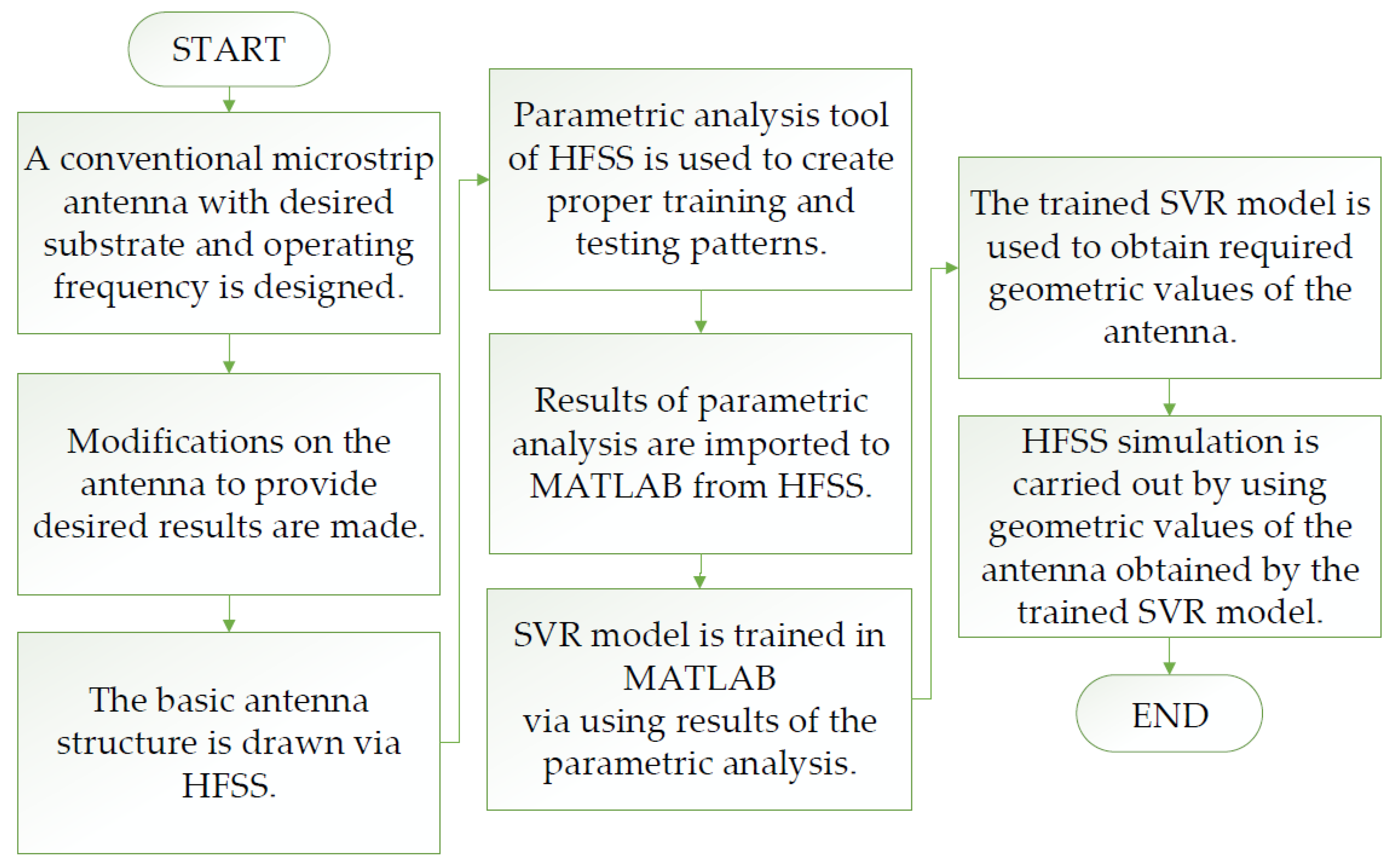
The design procedure is explained within a flow chart in Figure 2.

4. Simulation and Implementation

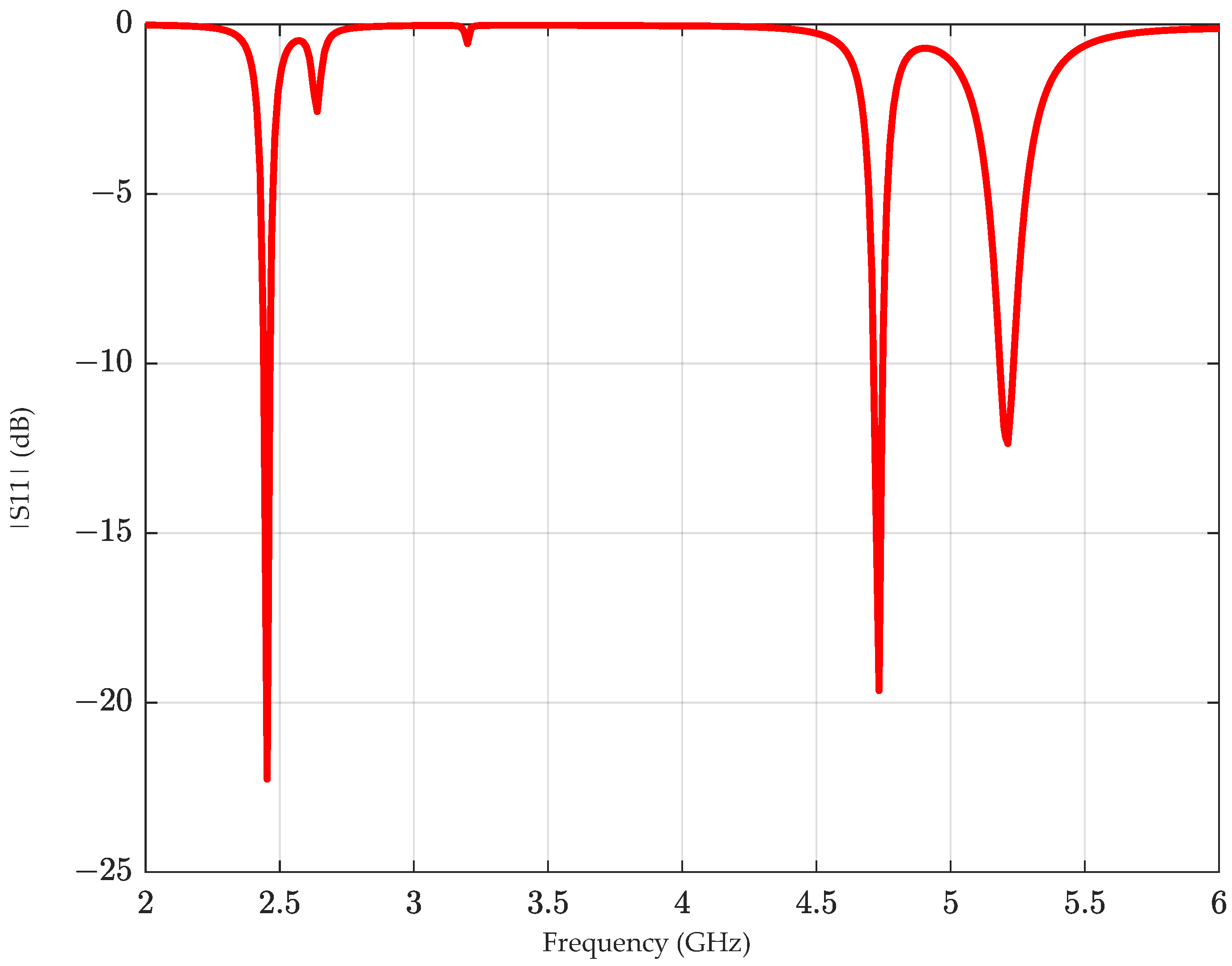
HFSS simulation is carried out by using (sL1, sL2, sW1, and sW2) and (r) parameter values of the MPATSAT obtained by the trained SVR model in Section 3. |S11| plot of MPATSAT is illustrated in Figure 3. The obtained resonance frequencies are 2.45 GHz, 4.73 GHz, and 5.21 GHz. At these frequencies, the 10 dB bandwidths are obtained as 20 MHz, 40 MHz, and 50 MHz, respectively.
Three-dimensional realized gain diagrams of MPATSAT for 2.45 GHz, 4.73 GHz, and 5.21 GHz are shown in Figure 4a–c, respectively. The maximum realized antenna gains are obtained as 6.1 dB, 4.6 dB, and 7.21 dB.
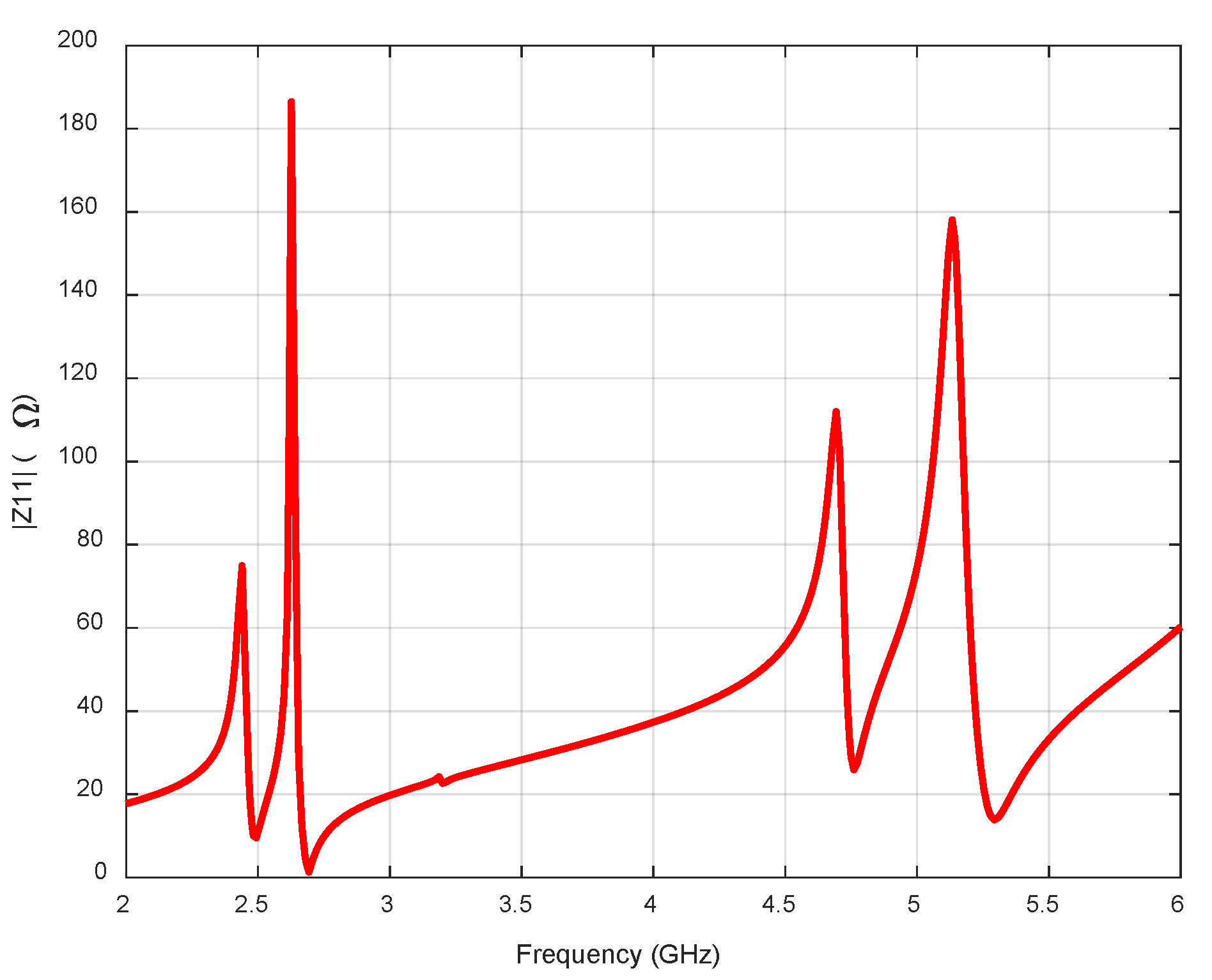
|Z11| parameter plot of MPATSAT is given in Figure 5. Input impedances were tuned to ~50 Ω for resonance frequencies. Input impedances are 47.45 Ω, 44.80 Ω, and 47.02 for 2.45 GHz, 4.73 GHz, and 5.21 GHz, respectively.
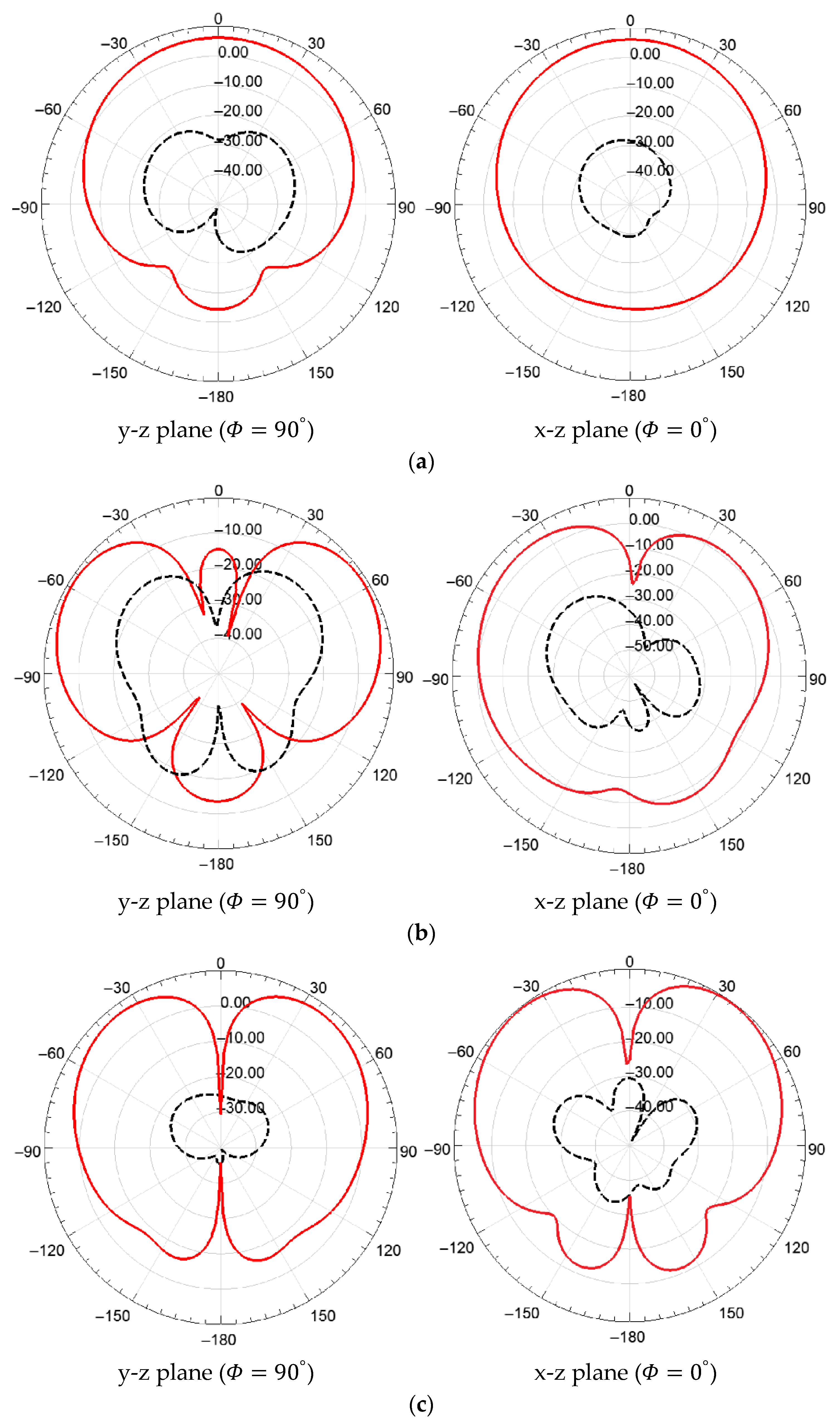
The co-polarization (co-pol.) and cross-polarization (cross-pol.) are very important from the application point of view to analyze the performance of antennas. In Figure 6a–c, co-pol. and cross-pol. radiation diagrams of MPATSAT are shown in the y–z plane and x–z plane for 2.45 GHz, 4.73 GHz, and 5.21 GHz, respectively.
Current distributions at the surface of MPATSAT for 2.45 GHz, 4.73 GHz, and 5.21 GHz are shown in Figure 7a–c, respectively. Current flows that cause the radiations in resonance frequencies can clearly be seen in Figure 7.
Radiation efficiency is obtained as 96% for 2.45 GHz, 75% for 4.73 GHz, and 98% for 5.21 GHz. Satisfactory radiation efficiency values are acquired at the resonance frequencies.
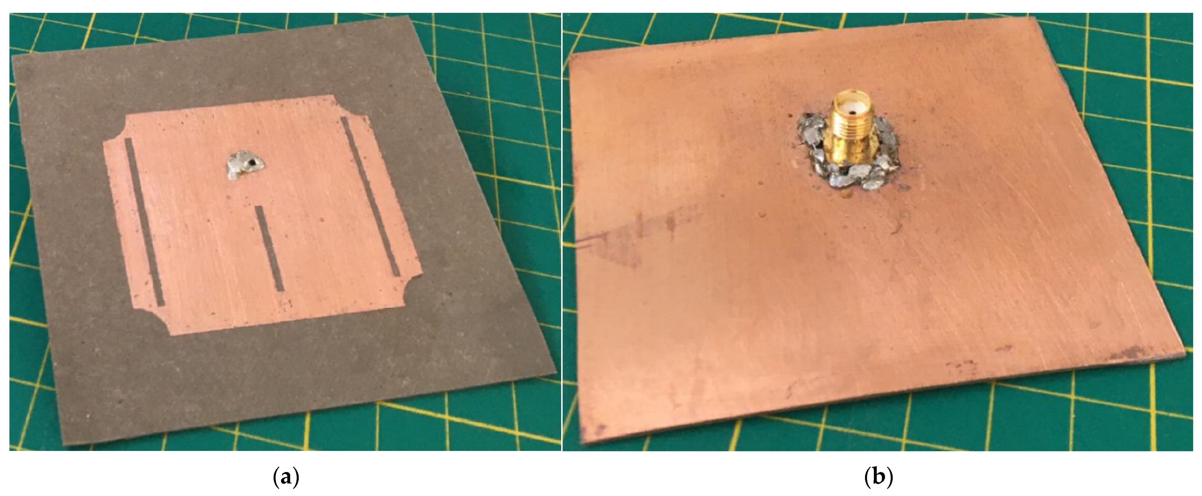
MPATSAT given in Figure 1a,b was implemented by using Rogers RT/duroid 5870 with relative permittivity of 2.33 and substrate thickness of 0.787 mm and antenna geometric values given above. The top and bottom views of the implemented MPATSAT are presented in Figure 8a,b, respectively. The soldering in Figure 8 is implemented by hand in a classical way. After connections are tested via a Multimeter, no connection problem was detected between the outer conductor-antenna ground and inner conductor-antenna patch. |S11| plot of the implemented MPATSAT is obtained by a network analyzer.
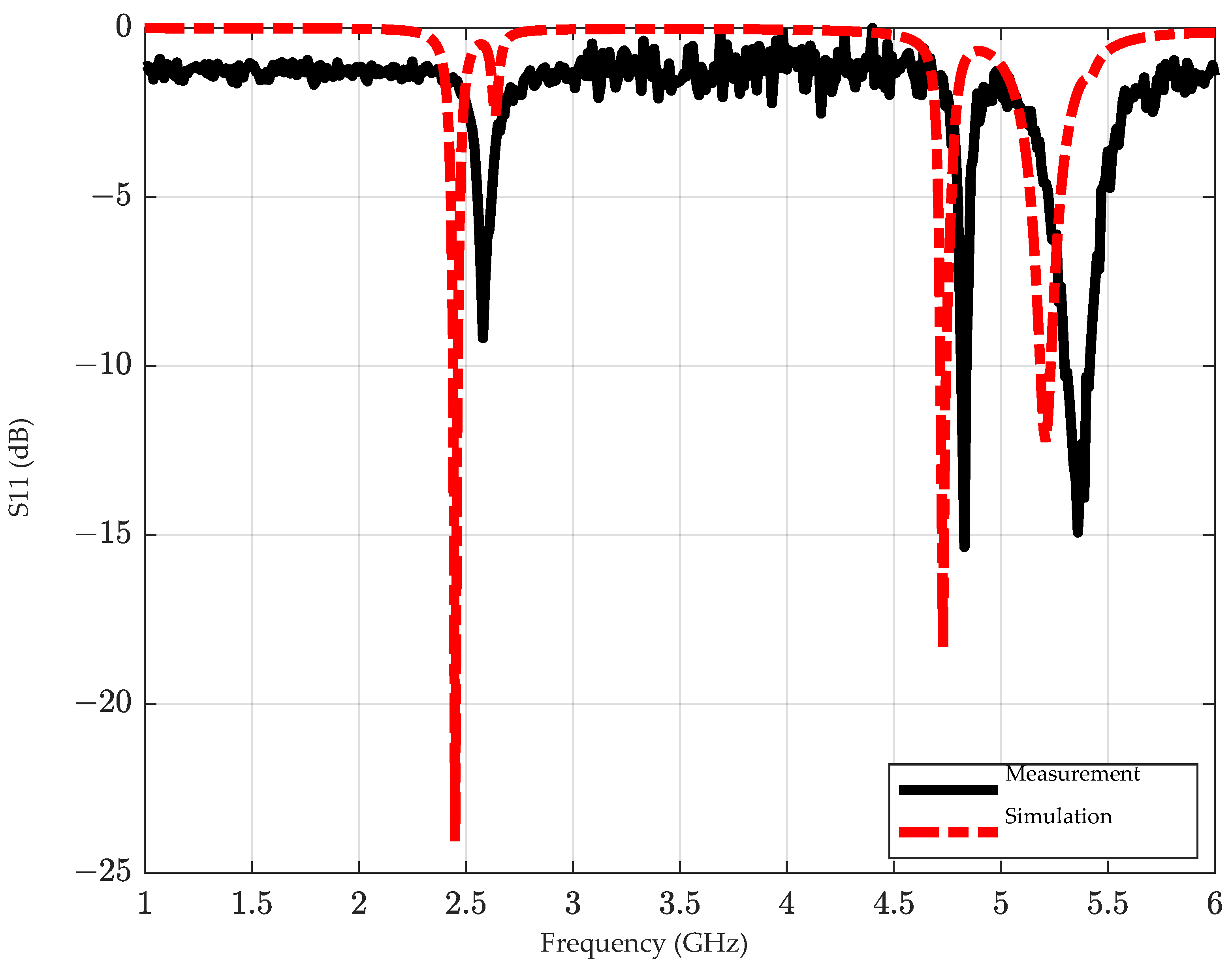
A comparison of |S11| plots of the simulation and measurement results is given in Figure 9. It can be observed that the simulation and measurement results coincide with each other approximately. The difference between simulation and measurement is due to measurement and implementation errors. The measured maximum antenna gains at the measured resonance frequencies are 3.1 dB, 3.8 dB, and 7.1 dB, respectively.
Table 3 shows the comparison of the antenna designed by the proposed method with several triple-band antennas given in the literature [55,56,57,58,59,60,61,62]. In terms of antenna gains, MPATSAT gives relatively better results. It should be noted that these antennas given in the literature were not designed with soft computation techniques.

5. Antenna Design via HFSS Optimization Tool

In order to compare the results attained by the SVR method, the HFSS optimization tool was also used in this paper. The required time during the optimization and accuracy of the simulation results from the desired values are selected as the main comparison parameters. HFSS optimization tool includes various types of optimization methods such as gradient- and search-based algorithms.
In this study, Genetic Algorithm (GA) [3,4,5,6,7,8] and Pattern Search (PS) [63,64,65] methods were used as optimizer in the HFSS optimization setup. Goal parameters are selected as the magnitude of S11 in dB values at f r 1 = 2.4 GHz, f r 2 = 4.7 GHz, and f r 3 = 5.3 GHz. Goal values are chosen to be less than or equal to −10 dB at these resonance frequencies. HFSS optimizer options are given in Table 4 for GA and PS. The same sampling strategy with the SVR model was used in the HFSS optimizer that is given in Table 1.
It can be observed that at the 715th iteration, the GA optimizer of HFSS obtained the optimal results. At the end of the optimization process via GA HFSS optimization tool, slot and arc truncation values are obtained as sW1 and sW2 = 1.8 mm, sL1 = 25.5 mm, sL2 = 12.75 mm and r = 1.36 mm via HFSS optimization with GA optimizer. Resonance frequencies with these antenna geometric parameters are obtained as 2.37 GHz, 4.52 GHz, and 5.17 GHz by HFSS simulation. The maximum realized antenna gains are 5.9 dB, 3.5 dB, and 6.6 dB, respectively, for these resonance frequencies.
PS HFSS optimizer obtained the optimal results at the 625th iteration. Slot and arc truncation values are obtained as sW1 and sW2 = 3.23 mm, sL1 = 21.34 mm, sL2 = 10.67 mm, and r = 1.0 mm via HFSS optimization with PS optimizer. Resonance frequencies are obtained as 2.33 GHz, 4.54 GHz, and 5.38 GHz by HFSS simulation. The maximum realized antenna gains are 5.6 dB, 2.8 dB, and 6.5 dB, respectively, for the resonance frequencies.
Simulation results obtained by the SVR model approach given in Section 3 and Section 4 were compared with the results obtained with HFSS optimizations; the comparison is provided in Table 5. Computation time for the SVR model is the required time for obtaining training and testing patterns via HFSS parametric simulation given in Section 3, and computation time for HFSS optimization is the total optimization time required by the HFSS optimization tool, as presented in Table 5. Computed resonance frequencies for the SVR model are given in Figure 3 of Section 4. Computed maximum realized gains at the resonance frequencies are given in Figure 4 of Section 4.
In Table 5, TAE denotes the total absolute error, and it is used to evaluate the accuracy of the methods used in this paper. TAE for resonance frequencies can be calculated by:
T A E f = | f r 1 d f r 1 c | + | f r 2 d f r 2 c | + | f r 3 d f r 3 c   |
where f r 1 d , f r 2 d , and f r 3 d are the desired resonance frequencies; and f r 1 c , f r 2 c , and f r 3 c are the computed resonance frequencies.

6. Conclusions

In this paper, one of the soft computing methods, Support Vector Regression (SVR), was used to design a triple-band antenna with the desired resonance frequency and gain. The SVR model was utilized to obtain the optimal values for the geometric parameters of an antenna that provides the desired antenna variables. A microstrip patch antenna with triple slots and arc-truncation (MPATSAT) was simulated using these values via High-Frequency Structural Simulator (HFSS), and simulation and measurement results were compared. The performance characteristics of MPATSAT were compared with those obtained for several antennas given in the literature. Then, the antenna was redesigned by using the optimization tools in HFSS with the same desired antenna parameter values. The SVR approach and HFSS optimization method were compared with respect to accuracy and required computation time. These comparison results justify the superiority of the proposed design approach.

Author Contributions

Conceptualization, T.G. and M.E.Y.; methodology, T.G. and M.E.Y.; software, G.Ö.G. and M.E.Y.; validation, T.G., M.E.A. and M.E.Y.; investigation, M.E.Y. and M.E.A.; resources, T.G., G.Ö.G. and M.E.A.; writing—original draft preparation, M.E.Y.; writing—review and editing, G.Ö.G., T.G., M.E.A. and M.E.Y.; visualization, T.G. and M.E.Y.; supervision, T.G. All authors have read and agreed to the published version of the manuscript.

Funding

This research received no external funding.

Institutional Review Board Statement

Not applicable.

Informed Consent Statement

Not applicable.

Data Availability Statement

Not applicable.

Conflicts of Interest

The authors declare no conflict of interest.

References

  1. Zadeh, L.A. Soft computing and fuzzy logic. IEEE Softw. 1994, 11, 48–56. [Google Scholar] [CrossRef]
  2. Zadeh, L.A. Fuzzy logic = computing with words. IEEE Trans. Fuzzy Syst. 1996, 4, 103–111. [Google Scholar] [CrossRef] [Green Version]
  3. Goldberg, D.E. Genetic Algorithms in Search, Optimization and Machine Learning Reading; Addison-Wesley: Boston, MA, USA, 1989. [Google Scholar]
  4. Haupt, R.L. An introduction to genetic algorithms for electromagnetics. IEEE Antennas Propag. Mag. 1995, 37, 7–15. [Google Scholar] [CrossRef] [Green Version]
  5. Weile, D.S.; Michielssen, E. Genetic algorithm optimization applied to electromagnetics: A review. IEEE Trans. Antennas Propag. 1997, 45, 343–353. [Google Scholar] [CrossRef]
  6. Johnson, J.M.; Rahmat-Samii, V. Genetic algorithms in engineering electromagnetics. IEEE Antennas Propag. Mag. 1997, 39, 7–21. [Google Scholar] [CrossRef] [Green Version]
  7. Haupt, R.L.; Werner, D.H. Genetic Algorithm in Electromagnetics; Wiley-Interscience: Hoboken, NJ, USA, 2007. [Google Scholar]
  8. Haupt, R.L. Thinned arrays using genetic algorithms. IEEE Trans. Antennas Propag. 1994, 42, 993–999. [Google Scholar] [CrossRef]
  9. Kennedy, J.; Eberhart, R. Particle swarm optimization. In Proceedings of the ICNN’95—International Conference on Neural Networks, Perth, WA, Australia, 27 November–1 December 1995. [Google Scholar] [CrossRef]
  10. Robinson, J.; Rahmat-Samii, Y. Particle swarm optimization in electromagnetics. IEEE Trans. Antennas Propag. 2004, 52, 397–407. [Google Scholar] [CrossRef]
  11. Boeringer, D.W.; Werner, D.H. Particle swarm optimization versus genetic algorithms for phased array synthesis. IEEE Trans. Antennas Propag. 2004, 52, 771–779. [Google Scholar] [CrossRef]
  12. Taguchi, G.; Chowdury, S.; Wu, Y. Taguchi’s Quality Engineering Handbook; Wiley-Interscience: Hoboken, NJ, USA, 2005. [Google Scholar]
  13. Boyd, S.; Vandenberghe, L. Convex Optimization; Cambridge University Press: Cambridge, UK, 2004; Available online: https://web.stanford.edu/~boyd/cvxbook/bv_cvxbook.pdf (accessed on 8 October 2022).
  14. Tsai, J.-T.; Liu, T.-K.; Chou, J.-H. Hybrid Taguchi-genetic algorithm for global numerical optimization. IEEE Trans. Evol. Comput. 2004, 8, 365–377. [Google Scholar] [CrossRef]
  15. Afsari, A.; Abbosh, A.; Rahmat-Samii, Y. Adaptive beamforming by compact arrays using evolutionary optimization of Schelkunoff polynomials. IEEE Trans. Antennas Propag. 2022, 70, 4485–4497. [Google Scholar] [CrossRef]
  16. Weng, W.; Yang, F.; Elsherbeni, A.Z. Linear antenna array synthesis using Taguchi’s method: A novel optimization technique in electromagnetics. IEEE Trans. Antennas Propag. 2007, 55, 723–730. [Google Scholar] [CrossRef]
  17. Günel, T.; Aydemir, E. Application of continuous parameter genetic algorithm to the problem of synthesizing bandpass distributed amplifiers. AEU-Int. J. Electron. Commun. 2002, 56, 351–354. [Google Scholar] [CrossRef]
  18. Günel, T.; Yiğit, M.E.; Günel, G.Ö. Genetic-based approach to the synthesis of rectangular microstrip antenna elements with reduced mutual coupling. In Proceedings of the 2018 International Symposium on Advanced Electrical and Communication Technologies (ISAECT), Rabat, Morocco, 21–23 November 2018. [Google Scholar] [CrossRef]
  19. Vapnik, V.N. An overview of statistical learning theory. IEEE Trans. Neural Netw. 1999, 10, 988–999. [Google Scholar] [CrossRef] [PubMed] [Green Version]
  20. Haykin, S. Neural Networks and Learning Machines, 3rd ed.; Pearson Prentice Hall: Hoboken, NJ, USA, 2009. [Google Scholar]
  21. Khan, T.; De, A. Modeling of microstrip antennas using neural networks techniques: A review. Int. J. RF Microw. Comp. Aid. Eng. 2015, 25, 747–757. [Google Scholar] [CrossRef]
  22. Khan, T.; De, A. Prediction of slot-shape, slot-size and inserted air-gap of a microstrip antenna using knowledge-based neural network. Prog. Electromagn. Res. C 2016, 65, 23–32. [Google Scholar] [CrossRef] [Green Version]
  23. Jain, S.K. Bandwidth enhancement of patch antennas using neural network dependent modified optimizer. Int. J. Microw. Wirel. Technol. 2016, 8, 1111–1119. [Google Scholar] [CrossRef]
  24. Aneesh, M.; Singh, A.; Ansari, J.A.; Kamakshi; Sayeed, S.S. Investigations for performance improvement of X-shaped RMSA using artificial neural network by predicting slot size. Prog. Electromagn. Res. C 2014, 47, 55–63. [Google Scholar] [CrossRef] [Green Version]
  25. Günel, T. Combination of artificial neural network model with genetic algorithm for the synthesis of microstrip radial stub. AEU-Int. J. Electron. Commun. 2000, 54, 241–243. [Google Scholar]
  26. Aşık, U.; Günel, T.; Erer, I. A wavelet-based radial basis function neural network approach to the inverse scattering of conducting cylinders. Microw. Opt. Technol. Lett. 2004, 41, 506–510. [Google Scholar] [CrossRef]
  27. Guney, K.; Sarikaya, N. A hybrid method based on combining artificial neural network and fuzzy inference system for simultaneous computation of resonant frequencies of rectangular, circular, and triangular microstrip antennas. IEEE Trans. Antennas Propag. 2007, 55, 659–668. [Google Scholar] [CrossRef]
  28. Cortes, C.; Vapnik, V. Support vector network. Mach. Learn. 1995, 20, 273–297. [Google Scholar] [CrossRef]
  29. Cai, J.; King, J.; Yu, C.; Liu, J.; Sun, L. Support vector regression-based behavioral modeling technique for RF power transistors. IEEE Microw. Wirel. Compon. Lett. 2018, 28, 428–430. [Google Scholar] [CrossRef]
  30. Xu, J.; Jiang, W.; Ma, L.; Li, M.; Yu, Z.; Geng, Z. Augmented time-delay twin support vector regression-based behavioral modeling for digital predistortion of RF power amplifier. IEEE Access 2019, 7, 59832–59843. [Google Scholar] [CrossRef]
  31. Wu, Y.; Tang, Z.; Xu, Y.; Guo, Y.; Zhang, B. Support vector regression for measuring electromagnetic parameters of magnetic thin-film materials. IEEE Trans. Magn. 2007, 43, 4071–4075. [Google Scholar] [CrossRef]
  32. Angiulli, G.; Cacciola, M.; Versaci, M. Microwave devices and antennas modelling by support vector regression machines. In Proceedings of the 2006 12th Biennial IEEE Conference on Electromagnetic Field Computation, Miami, FL, USA, 30 April–3 May 2006. [Google Scholar] [CrossRef]
  33. Tokan, N.T.; Gunes, F. Support vector design of the microstrip antenna. In Proceedings of the 2008 IEEE 16th Signal Processing, Communication and Applications Conference, Aydin, Turkey, 20–22 April 2008. [Google Scholar] [CrossRef]
  34. Roy, C.; Khan, T.; Kanaujia, B. Performance parameters prediction of slotted microstrip antennas with modified ground plane using support vector machine. Int. J. Microw. Wirel. Technol. 2016, 9, 1169–1177. [Google Scholar] [CrossRef]
  35. Yiğit, M.E.; Günel, T.; Günel, G.Ö. PSO based approach to the synthesis of a cylindrical-rectangular ring microstrip conformal antenna using SVR models with RBF and wavelet kernels. In Proceedings of the 2018 18th Mediterranean Microwave Symposium (MMS), Istanbul, Turkey, 31 October–2 November 2018. [Google Scholar] [CrossRef]
  36. Dai, X.W.; Mi, D.L.; Wu, H.T.; Zhang, Y.H. Design of Compact Patch Antenna Based on Support Vector Regression. Radioengineering 2022, 31, 339–345. [Google Scholar] [CrossRef]
  37. Ansys, HFSS 3D High Frequency Simulation Software. Available online: https://www.ansys.com/products/electronics/ansys-hfss (accessed on 8 October 2022).
  38. Dassault Systems, CST Studio Suite Electromagnetic Field Simulation Software. Available online: https://www.3ds.com/products-services/simulia/products/cst-studio-suite (accessed on 8 October 2022).
  39. Cadence, AWR Software Microwave Office. Available online: https://www.awr.com/awr-software/products/microwave-office (accessed on 8 October 2022).
  40. Verma, S.; Ansari, J.A.; Singh, A. Truncated equilateral triangular microstrip antenna with and without superstrate. Wirel. Pers. Commun. 2017, 95, 873–889. [Google Scholar] [CrossRef]
  41. Nirate, S.; Vani, R.M.; Hunagund, P.V.; Mallikarjun, S.L. Arc truncated suspended rectangular microstrip antenna. Int. J. Adv. Res. Electr. Electron. Instrum. Eng. 2016, 5, 1771–1775. [Google Scholar]
  42. Kumar, S.; Dixit, A.S.; Malekar, R.R.; Raut, H.D.; Shevada, L.K. Fifth generation antennas: A comprehensive review of design and performance enhancement techniques. IEEE Access 2020, 8, 163568–163593. [Google Scholar] [CrossRef]
  43. Iplikci, S. Online trained support vector machines-based generalized predictive control of non-linear systems. Int. J. Adapt. Control. Signal Processing 2006, 20, 599–621. [Google Scholar] [CrossRef]
  44. Smola, A.J.; Schölkopf, B. A tutorial on support vector regression. Stat. Comput. 2004, 14, 199–222. [Google Scholar] [CrossRef] [Green Version]
  45. Cristianini, N.; Shawe-Taylor, J. An Introduction to Support Vector Machines and Other Kernel-Based Learning Methods; Cambridge University Press: Cambridge, UK, 2000. [Google Scholar]
  46. Iplikci, S. A comparative study on a novel model-based PID tuning and control mechanism for nonlinear systems. Int. J. Robust Nonlinear Control 2009, 20, 1483–1501. [Google Scholar] [CrossRef]
  47. Hou, S.; Zhou, Y.; Liu, H.; Zhu, N. Wavelet support vector machine algorithm in power analysis attacks. Radioengineering 2017, 26, 890–902. [Google Scholar] [CrossRef]
  48. Zhang, L.; Zhou, W.; Jiao, L. Wavelet support vector machine. IEEE Trans. Syst. Man Cybern. Part B Cybern. 2004, 34, 34–39. [Google Scholar] [CrossRef] [Green Version]
  49. Parikh, U.B.; Das, B.; Maheshwari, R.P. Combined wavelet-SVM technique for fault zone detection in a series compensated transmission line. IEEE Trans. Power Deliv. 2008, 23, 1789–1794. [Google Scholar] [CrossRef]
  50. Du, P.; Tan, K.; Xing, X. Wavelet SVM in reproducing kernel Hilbert space for hyperspectral remote sensing image classification. Opt. Commun. 2010, 283, 4978–4984. [Google Scholar] [CrossRef]
  51. Balanis, C.A. Antenna Theory Analysis and Design, 3rd ed.; John Wiley & Sons, Inc.: Hoboken, NJ, USA, 2005. [Google Scholar]
  52. Haneishi, M.; Yoshida, S. A design method of circularly polarized rectangular microstrip antenna by one-point feed. Electron. Comm. Jpn. Part I 1981, 64, 46–54. [Google Scholar] [CrossRef]
  53. Mathew, S.; Anitha, R.; Deepak, U.; Aanandan, C.K.; Mohanan, P.; Vasudevan, K. A Compact tri-band dual-polarized corner-truncated sectoral patch antenna. IEEE Trans. Antennas Propag. 2015, 63, 5842–5845. [Google Scholar] [CrossRef]
  54. Mathworks, MATLAB. Available online: https://www.mathworks.com/products/matlab.html (accessed on 9 September 2022).
  55. Parveen, T.; Khan, Q.U.; Fazal, D.; Ali, U.; Akhtar, N. Design and analysis of triple band circular patch antenna. AEU-Int. J. Electron. Commun. 2019, 112, 152960. [Google Scholar] [CrossRef]
  56. Li, Y.; Yu, W. A miniaturized triple band monopole antenna for WLAN and WIMAX applications. Int. J. Antennas Propag. 2015, 2015, 146780. [Google Scholar] [CrossRef] [Green Version]
  57. Li, L.; Zhang, X.; Yin, X.; Zhou, L. A compact triple-band printed monopole antenna for WLAN/WiMAX applications. IEEE Antennas Wirel. Propag. Lett. 2016, 15, 1853–1855. [Google Scholar] [CrossRef]
  58. Zheng, Y.; Wang, P.; Hua, M.; Gao, P. Compact triple-band monopole antenna for WLAN/WiMAX applications. IEICE Electron. Express 2013, 10, 20130638. [Google Scholar] [CrossRef] [Green Version]
  59. Paul, P.M.; Kandasamy, K.K.; Sharawi, M.S. A tri-band slot antenna loaded with split ring resonators. Microw. Opt. Technol. Lett. 2017, 59, 2638–2643. [Google Scholar] [CrossRef]
  60. Sarkar, D.; Saurav, K.; Srivastava, K.V. Multi-band microstrip-fed slot antenna loaded with a split-ring resonator (SRR). Electron. Lett. 2014, 50, 1498–1500. [Google Scholar] [CrossRef]
  61. Li, H.; Du, J.; Yang, X.-X. Compact triple-band wearable circular patch antenna for WLAN/WiMAX applications. In Proceedings of the 2021 International Symposium on Antennas and Propagation (ISAP), Taipei, Taiwan, 19–22 October 2021. [Google Scholar] [CrossRef]
  62. Maity, B.; Nayak, S.K. Design of compact microstrip-fed triple-band slot antenna with defected ground structure for wireless communications. J. Electromagn. Waves Appl. 2022, 36, 1702–1716. [Google Scholar] [CrossRef]
  63. Hooke, R.; Jeeves, T.A. Direct search solution of numerical and statistical problems. J. ACM 1961, 8, 212–229. [Google Scholar] [CrossRef]
  64. Torczon, V. On the Convergence of pattern search algorithms. SIAM J. Optim. 1997, 7, 1–25. [Google Scholar] [CrossRef]
  65. Gardeux, V.; Omran, M.G.H.; Chelouah, R.; Siarry, P.; Glover, F. Adaptive pattern search for large-scale optimization. Appl. Intell. 2017, 45, 319–330. [Google Scholar] [CrossRef]
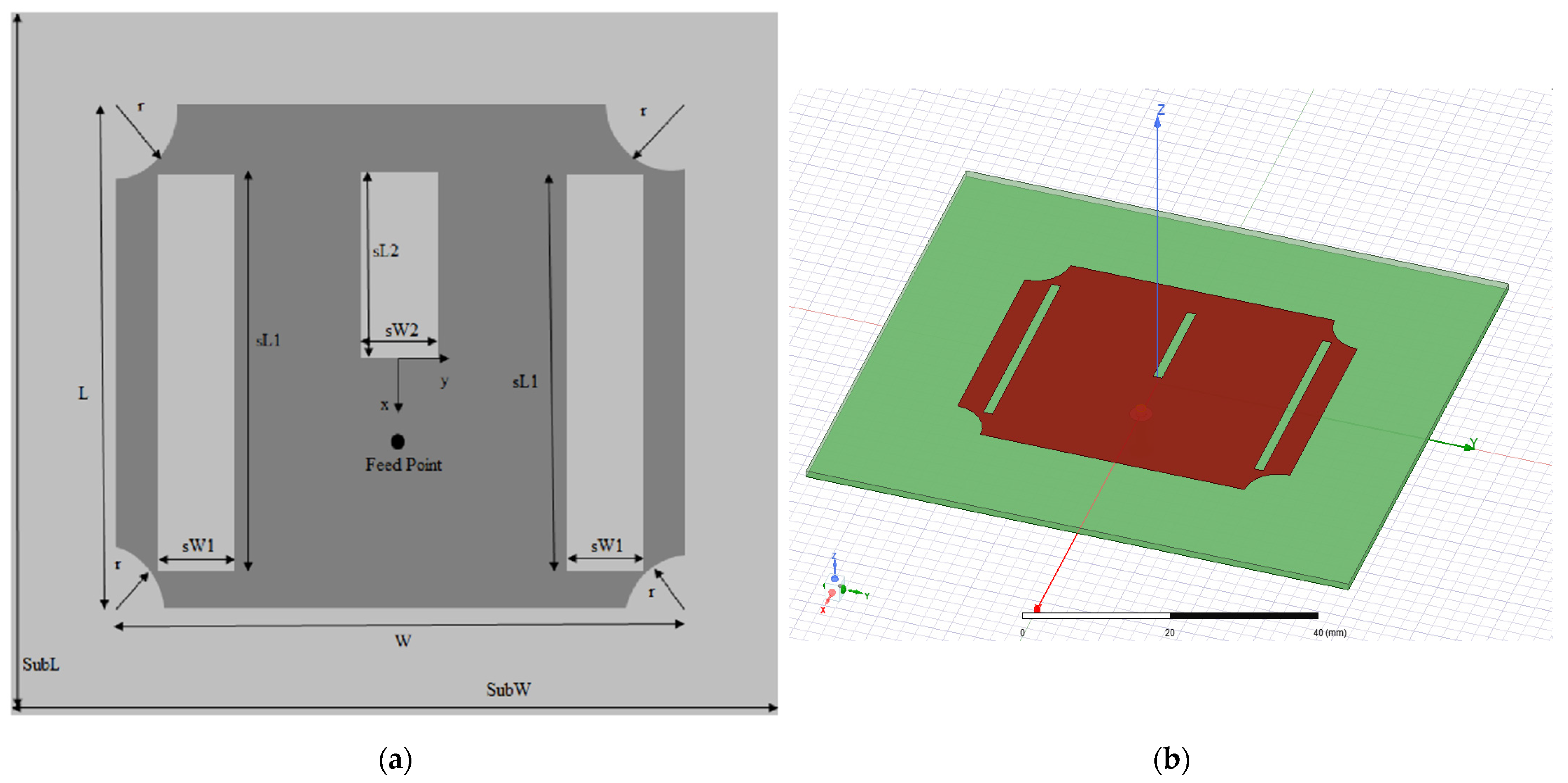
Figure 1. Drawings of the proposed antenna: (a) general schematic representation of MPATSAT; (b) sketch of MPATSAT in HFSS.
Applsci 12 11923 g001
Figure 2. Flow chart of the design procedure.
Applsci 12 11923 g002
Figure 3. |S11| plot of MPATSAT.
Applsci 12 11923 g003
Figure 4. Three-dimensional realized gain diagrams of MPATSAT: (a) for 2.45 GHz; (b) for 4.73 GHz; (c) for 5.21 GHz.
Applsci 12 11923 g004
Figure 5. |Z11| plot of MPATSAT.
Applsci 12 11923 g005
Figure 6. Co-pol. () and cross-pol. (---) radiation diagrams of MPATSAT in y–z ( Φ = 90 ° ) and x–z plane ( Φ = 0 ° ): (a) for 2.45 GHz; (b) for 4.73 GHz; (c) for 5.21 GHz.
Applsci 12 11923 g006
Figure 7. Current distributions at the surface of MPATSAT: (a) for 2.45 GHz; (b) for 4.73 GHz; (c) for 5.21 GHz.
Applsci 12 11923 g007
Figure 8. Implemented MPATSAT: (a) Top view; (b) Bottom view.
Applsci 12 11923 g008
Figure 9. Comparison of |S11| plots of the simulation and the measurement.
Applsci 12 11923 g009
Table 1. Sampling procedure for training and testing.
VariablesIntervals and Number of Samples
slot Width 1 (sW1) 0.5   mm s W 1 10   mm
slot Width 2 (sW2) 0.5   mm s W 2 10   mm
slot Length 1 (sL1) 10   mm s L 1 30   mm
slot Length 2 (sL2) 0.5   mm s L 2 15   mm
radius of arc-truncation (r) 0.5   mm r 5   mm
number of training samples1100
number of testing samples149
total number of samples1249
Table 2. SVR model parameters.
SVR ParametersSelected Kernel Function Type and Parameter Values
Kernel functionMexican-hat wavelet (19)
C2 × 1012
ε5 × 10⁻⁴
a2.97
Table 3. Comparison of performance characteristics of MPATSAT with several antennas given in the literature.
MPATSAT[55][56][57][58][59][60][61][62]
number of bandstripletripletripletripletripletripletripletripletriple
antenna dimensions L × W (mm)47.5 × 38.627 (radius)34 × 1820 × 2129 × 1060 × 6040 × 5060 × 6044 × 45
substrateRT Duroid 5870RT Duroid 5870FR-4FR-4FR-4FR-4FR-4denimFR-4
substrate thickness (mm)0.7871.51.61.571.61.560.811.6
resonance (operating) frequencies (GHz)2.5
4.8
5.3
1.8
2.4
5.4
2.5
3.5
5.5
1.29
2.44
3.26
2.4
3.5
5.5
2.6
4.2
4.6
1.65
1.93
2.2
2.45
3.25
5.8
2.39
3.55
4.13
bandwidths (MHz)20
40
50
-300
300
1000
210
300
1390
80
420
600
580
120
100
70
60
280
76
156
328
196
110
220
gains at resonance frequencies (dB)3.1
3.8
7.1
5.5
7.8
7.9
0.28
1.42
4.76
1.29
2.44
3.26
~1.75
~2
~2.3
4.4
3.9
3.8
1.08
1.82
2.93
0.025
−1.871
3.703
4.05
2.52
2.15
Table 4. HFSS optimizer options for Genetic Algorithm and Pattern Search.
ParameterGAPS
number of parents (current gen.)30-
number of mates30-
number of children30-
crossover typesimulated binary-
mutation typepolynomial-
number of survivors10-
number of individuals (next gen.)30-
selection typeroulette-
selection pressure10-
maximum number of iterations10001000
mutation probability0.01-
crossover probability0.98-
cost function norm typeL1L1
weights11
Table 5. Comparison of results of SVR model and HFSS optimization tool.
SVR Model
Approach
HFSS Optimization
Tool (GA)
HFSS Optimization
Tool (PS)
computation time2 h and
36 min
9 h and
46 min
7 h and
32 min
TAEf (GHz) (24)0.170.340.31
desired resonance
frequencies (GHz)
2.4
4.7
5.3
2.4
4.7
5.3
2.4
4.7
5.3
computed resonance frequencies (GHz)2.45
4.73
5.21
2.37
4.52
5.17
2.33
4.54
5.38
computed maximum realized gains at the resonance
frequencies (dB)
6.1
4.6
7.21
5.9
3.5
6.6
5.6
2.8
6.5
Publisher’s Note: MDPI stays neutral with regard to jurisdictional claims in published maps and institutional affiliations.