Article

Multiscale Backcast Convolution Neural Network for Traffic Flow Prediction in The Frequency Domain

1
College of Urban Rail Transit and Logistics, Beijing Union University, Beijing 100101, China
2
Beijing Key Laboratory of Information Service Engineering, Beijing Union University, Beijing 100101, China
*
Authors to whom correspondence should be addressed.
Appl. Sci. 2022, 12(23), 11912; https://doi.org/10.3390/app122311912
Submission received: 22 October 2022 / Revised: 11 November 2022 / Accepted: 14 November 2022 / Published: 22 November 2022
(This article belongs to the Section Transportation and Future Mobility)

Abstract

:
With the construction of intelligent transportation systems in recent years, intelligent methods for the prediction of traffic flow are becoming more and more important, and accurate prediction plays a key role in enabling downstream scheduling algorithms. However, the accuracy of most current forecasting algorithms remains unsatisfactory. Because traffic depends on the time of the day and varies throughout the week, such as during peak commuting periods as opposed to other times, traffic flow data show evident cyclical patterns. We capitalize on this notion and propose a multiscale convolutional feedback network for frequency prediction based on frequency angle. We combine multiscale convolution (MSC) with dilated convolution, and increase the convolutional receptive field by expanding cavity size while retaining similar parameterization costs, and achieve multiscale convolution with kernels referring to different receptive fields. At the same time, we incorporate an autoencoding module by assigning the same set of hidden features to input reconstruction and output prediction, which results in enhanced stability of features within the hidden layers. When we tested our approach on the Traffic dataset, our model achieved the best performance as assessed via the three indicators measured using mean squared error (MSE), mean absolute error (MAE), and correlation coefficient (CORR), with improvements of 3.818%, 2.472% and, 0.1515%, respectively.

1. Introduction

Recent economic developments worldwide have led to a steady increase in road traffic. Because many of the problems posed by the increase of traffic flow are difficult to solve, such as traffic jams, traffic accident and so on [1,2,3], intelligent transportation systems (ITS) have become increasingly important [4]. Current technology can maximize road utilization without changing the existing road structure, and various scheduling algorithms rely on traffic flow data, which can be accessed through various data mining algorithms. Traffic flow and calendar time are strongly coupled because traffic flow varies over different time periods, and can be treated as a natural time series. In addition, because traffic intersections are key nodes for analyzing traffic flow and different intersections are strongly coupled over space, traffic flow data are also characterized by spatial correlations. In summary, traffic flow data represent a form of spatially correlated time series data, and the prediction of traffic flow time series can guide the deployment of downstream processing algorithms.
In the last twenty years, a lot of traffic flow prediction approaches were proposed from different perspectives [5,6,7,8]. The traffic flow data is represented by time series data; hence, the most typical approaches used for traffic flow prediction are AutoRegressive based approaches [9,10,11]. The AutoRegressive based methods suppose that the prediction time stamp result is a linear combination of the past several time stamp values. This priori hypotheses works well in solving some simple prediction tasks but brings new problems at the same time, such as ignoring spatial correlation between multiple time series, unable to capture complex temporal varying mode, etc. Similarly, Support Vector Regression based approaches [12,13], another classical approach, faces a homologous problem. The accuracy of these classical approaches is relatively low due to the limited fitting and generalization ability of functions, especially for solving prediction tasks with a modern complex traffic flow time series dataset.
As the deep learning techniques develop, the fitting and generalization ability of learning system is greatly raised. In recent years, the methods used for traffic flow prediction have been mainly based on deep learning techniques operating over temporal and spatial dimensions, such as Feed-forward Neural Networks [14], Recurrent Neural Networks (RNN) [15], and Convolutional Neural Networks (CNN) [16]. After intense research and development, these networks have achieved good results in traffic flow prediction problems, as recently demonstrated by Bi-LSTM [17], StemGNN [18], and Autoformer [19]. These findings go far beyond traditional statistical methods, which are essentially focused on the time-domain patterns of sequences and attempt to predict future information from past point-in-time information. Notwithstanding the success of machine learning in this area, two main problems remain unresolved. First, traffic flow data are strongly cyclical (traffic flow is more intense than usual during the morning and evening rush hours, and less intense on weekends than on weekdays). This important feature is difficult to model directly via a time-domain representation. Second, RNN architectures based on time-domain information are greatly affected by the length of the input sequence (as the length increases, model performance decreases and inference time increases). To overcome these limitations, in this study, we eliminate the influence of time domain characteristics by operating our analysis in the frequency domain, and we propose a multiscale convolutional feedback network that is also based on the frequency domain. The core contributions of this article are the following:
  • This paper proposes a new prediction network based on a deep learning approach, which captures and learns the strong periodic pattern of traffic flow data by processing the frequency domain characteristics of traffic flow data. The network is integrated into a multiscale structure by combining dilated convolution modules of different sizes to increase network responsiveness to different frequency components and increase the robustness of network features. At the same time, inspired by the autoencoder structure and the N-BEATS network [20], our network is divided into a feedback branch and a prediction branch. The prediction branch is used to output the prediction result, while the feedback branch is used to fit the input sequence. This approach stabilizes features within hidden layers.
  • Our model outperformed four other models when challenged with the Traffic public dataset, delivering superior results in terms of Mean Squared Error (MSE), Mean Absolute Error (MAE), and Correlation coefficient (CORR). The role played by different model components was studied via ablation experiments.

2. Related Works

In recent years, traffic flow prediction methods based on deep learning have received more and more attention, and numerous new methods have emerged that build upon classical deep learning algorithms. The most basic methods, such as the LSTM [21] and GRU [22] models based on RNN architectures, are widely used in traffic flow prediction problems. Recent studies have focused on solving the gradient problem associated with LSTM and GRU models, and the problem of slow training speed, for example using effective attention mechanisms. Attention mechanisms were proposed to improve the accuracy of sequence-to-sequence (Seq2Seq) models [4] by assigning weights to features at different time steps. This was achieved by calculating similarity with a given metric (Key) to enhance the feature extraction capabilities of the model. For example, MTGNN [23] attempts to model multivariate time series through an attention mechanism operating over both temporal and spatial dimensions. Do et al. [24] establish the spatial-temporal correlation of sequences by combining convolutional gating recursive units with attention mechanisms. Cheng et al. [25] use attention mechanisms to model different series at adjacent intersections, known as sequential slots. They extract features from the upstream and downstream sequence slots of each target location, and then use the attention mechanism to assign weights to them. Xiao et al. [26] adopted LSTM in combination with the attention mechanism to extract time domain features and used convolutional layers to extract spatial features. Thanks to recent breakthroughs in applying the Transformer structure [27] to a wide range of deep learning tasks, its core module named the self-attention mechanism, has become an effective improvement on the standard attention mechanism. Unlike standard attention mechanisms, the similarity indicator (Key) used to support self-attention mechanisms is derived from a linear transformation of the input, hence the adoption of the term “self” to denote this class of attentional algorithms. Zhang et al. proposed SATP-GAN [28], which is based on self-attention mechanisms and generative adversarial networks (GAN). Their approach uses self-attention instead of an RNN structure to extract sequential time patterns and relies on reinforcement learning methods to adjust model parameters. Yan et al. [29] proposed a Traffic Transformer model that uses global and local encoders to improve transformers for traffic flow prediction problems. The latest time series forecasting model, Autoformer [19], has also achieved excellent performance on traffic flow dataset. This model incorporates a series-level autocorrelation mechanism based on autocorrelation theory to replace the self-attention mechanism, with the goal of capturing periodic information across the sequence more effectively.
In addition to the above methods, graph neural networks are also commonly used for traffic flow modeling. Graph neural networks are deep learning methods for processing graph data structures. They are better suited to describing the spatial relationships of roads than convolutional networks; the latter can only handle spatial relationships in Euclidean spaces represented by two-dimensional matrices or raster images, while graph neural networks [29] can represent non-Euclidean pairwise relationships in road networks. Through prior knowledge, self-learning, and other methods, it is possible to obtain a graph structure adjacency matrix between traffic intersections. This tool can be used to describe the degree of correlation between different intersections to explicitly model spatial relationships associated with traffic flow data. Seo et al. [30] propose a graph convolutional recursive network method that combines graph convolution with recurrent neural networks. Yu et al. [31] propose a graph convolutional neural network with a gating mechanism, which preserves the ability of the model to capture long-term temporal correlations. To more effectively reconstruct the adjacency matrix of the traffic flow data graph, StemGNN [18] exploits an attention mechanism to derive a relationship diagram for the intersection by encoding traffic flow data via the GRU unit. This unit is used to model the graph neural network and extract features in the frequency domain.

3. Model Architecture

This section describes the input data processing pipeline and the overall architecture of the multiscale convolutional feedback network operating in the frequency domain.

3.1. Problem Definition and Preprocessing

In this paper, all processing characteristics of the model are defined in the frequency domain. Problem definition and data flow are detailed below.
Given a multivariate time series X = x t i N × T , X is a real matrix, N is the number of variables, T is the length of time, and   x t i  x the value of the ith sequence at moment t. The prediction length is L:
W ¯ k = F X T = t = 0 T 1 x t i e i 2 π k K t W k = r e s h a p e W ¯ k V l = f W k V ¯ l = r e s h a p e 1 V l Y ^ L = F 1 V ¯ l = 1 L k = 0 L 1 V ¯ k e i 2 π k K l
F   is the Fourier transform, F 1 is the inverse Fourier transform, W ¯ k is a complex matrix containing the frequency representation of the input sequence X T . Taking advantage of the conjugate symmetry that characterizes the output of the Fourier transform, we only consider the half-side spectrum so k = T / 2 + 1 , where [*] is the rounding operation. Imaginary part and real part of the complex matrix are subsequently extracted via the r e s h a p e operation and stacked onto two-dimensional vectors in the form of real numbers. W k   is the converted real matrix. Taking one series with length T as an example, the preprocessing method is shown in Figure 1:
f is the learning target for the model, and the output of the model is in the same format as W k . The inverse of the r e s h a p e operation is used to convert V l into a complex matrix V ¯ l , which is then subjected to inverse Fourier transformation to obtain the final prediction result Y ^ L of length L .
In general, our goal is to obtain a frequency mapping model, which receives the frequency representation of the input time series and outputs the combination of the imaginary part and the real part of the prediction frequency. Thus, we can ignore the temporal features of input/output series to simplify our prediction problem.

3.2. Multiscale Backcast Convolution Neural Network

3.2.1. Dilated Multi-Scale Convolutional Layer

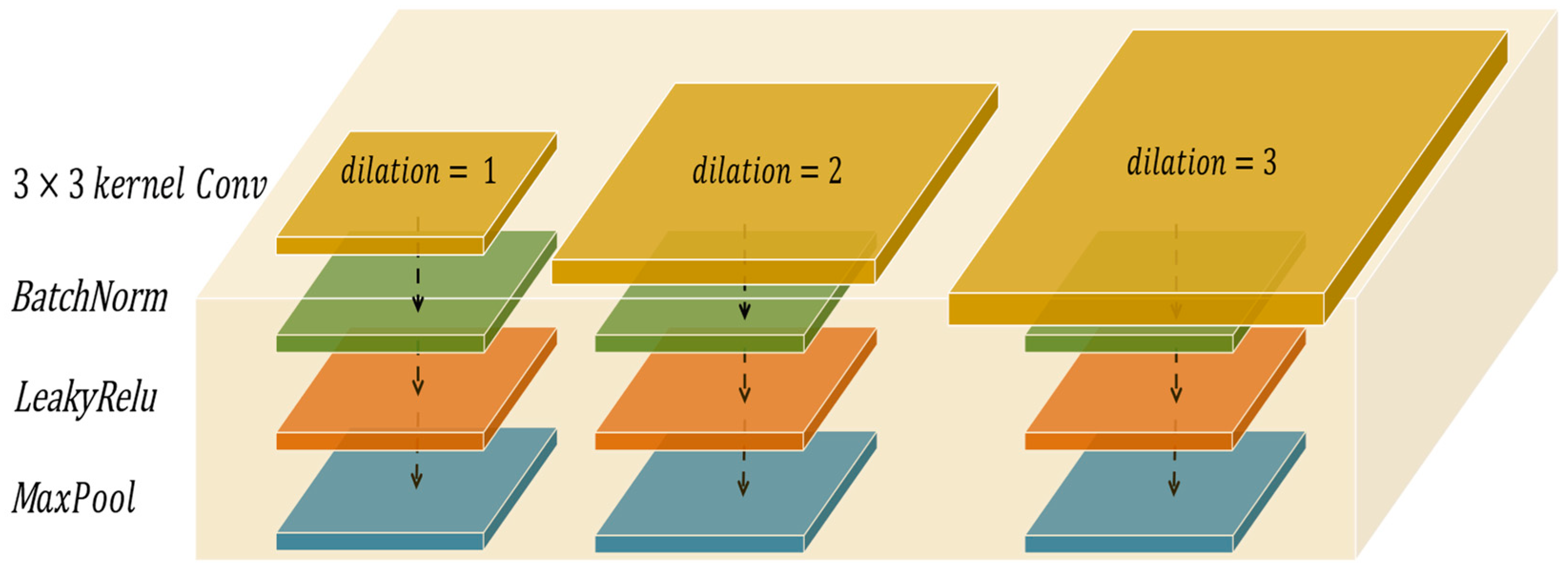
After the preprocessing method described in Section 3.1, the traffic flow time series of two-dimensional multivariate data, initially composed of variable dimensions and time dimensions, was transformed into three-dimensional data composed of variable dimensions, frequency dimensions, and complex dimensions. We denote this object with W k N × k × 2 , where 2 in the final dimension represents imaginary and real parts. Because the frequency domain representation of the time series records amplitude from low to high frequency, the different frequency components are not independent. In order to use as few parameters as possible to explore the dependencies between different frequency bands, we designed a multiscale convolutional feedback network for the frequency domain based on a two-dimensional convolution module. Multiscale convolution comes from the Inception Network [32], which uses multiple sizes of convolution kernels to extract features of different scales for the same set of feature maps, and then combines results across scales. This method can effectively improve the utilization rate of feature maps. Building on this approach, model parameters are further reduced by using dilated convolution [33] to enhance the receptive field of the convolutional kernel without increasing the number of parameters for convolutional kernels spanning multiple scales. The multiscale convolutional layer adopted in this paper is shown in Figure 2.
In the figure, dilation represents the size of the dilation. Each multiscale convolutional layer contains three convolutional kernels of different sizes. Size variation is generated by the size of the dilation, not by the size of the convolutional kernel. By increasing dilation size, the receptive field of the convolutional kernel can be expanded without altering the number of parameters associated with the convolutional kernel. The three convolutional layers use padding operations to keep the feature map size of the input and output unchanged. After that, the features are normalized using the BatchNorm layer. By using LeakyRelu as the activation function, and by downsampling the feature map using maximum pooling, we obtain feature maps for the three different receptive fields. It should be noted that the dimensions of the three sets of feature maps are the same.

3.2.2. Overall Architecture

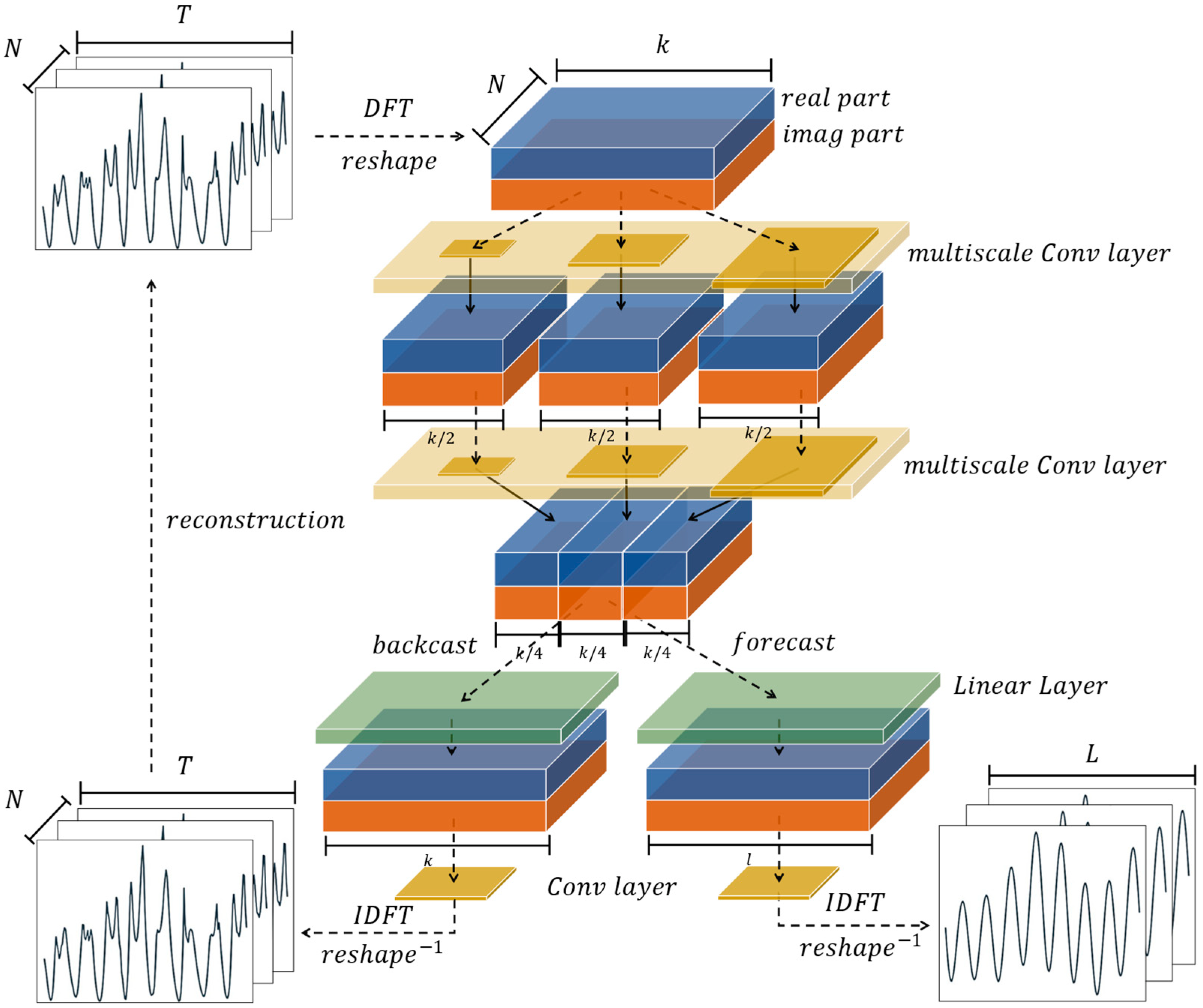
The overall architecture diagram of our model is shown in Figure 3. First, the input multivariate sequence X T N × T is transformed to obtain the frequency domain representation. Real and imaginary parts of the complex matrix are separated by the reverse operation to form a three-dimensional real matrix W k N × k × 2 , which is then used as input for the model. W k goes through the first multiscale convolutional layer to obtain a feature map of three sets with half frequency length:
U 1 1 , U 2 1 , U 3 1 = M u l t i s c a l e C o n v W k   U i 1 m × k 2 × 2   ,   i 1 ,   2 ,   3
In the above expression, m indicates the number of convolutional kernels in the convolutional layer, which is set to 512 for the experiments reported in this article. By applying a similar operation, we obtain a second multiscale convolutional layer U 1 2 , U 2 2 , U 3 2 with frequency length 4 / k .
After obtaining three sets of feature maps, we use the concatenation operation to connect the three sets of feature maps:
  U 3 = c o n c a t U 1 2 , U 2 2 , U 3 2 m × 3 × k 4 × 2
  U 3 is used as an encoding feature for forecasting. We are inspired by the Autoencoder and StemGNN [6], where the feedback branch and the prediction branch are used separately. First, the two branches expand or shorten the frequency length of   U 3 through their respective fully connected layers, to accommodate the requirements of both branches for their respective frequency bands:
U f o r e c a s t 4 = U 3 W f m × l × 2 ,  
U b a c k c a s t 4 = U 3 W b m × k × 2
W f and W b are learnable parameters. Following this step, the two sets of features are processed by the convolutional layer. The output is represented in the frequency domain, so it needs to be converted to the time domain via inverse Fourier transformation.
U b a c k c a s t 4 is used to reconstruct the X T of the input sequence to stabilize the hidden features of the model, while U f o r e c a s t 4 is used to predict the future. The errors of the two together constitute the training loss function:
loss = ( B t i X T x t i ) 2 + y ^ l i y l i 2
In the expression above, B t i X T is the reconstruction value of the ith variable output by the model backcasting at moment t, x t i is the input value of the simulcast, y ^ l i is the predicted value of the l-moment of the ith variable, and y l i is the real value of the simulcast. The result is added as the loss value of the model, and model parameters are optimized using the Adam optimizer [34].

4. Experiments and Analysis

4.1. Dataset and Evaluation Metrics

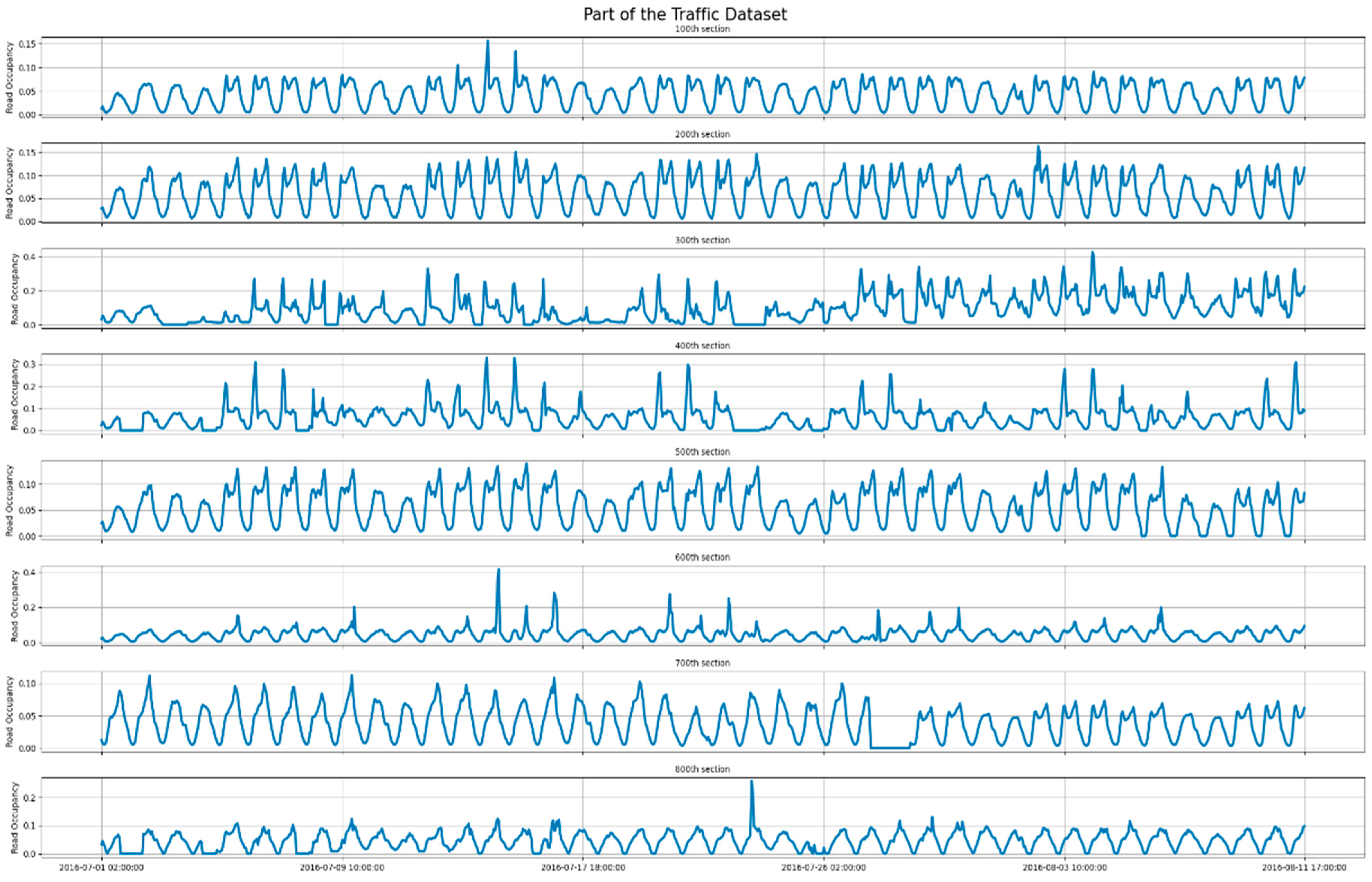
We used the public Traffic dataset from the California Department of Transportation as experimental input data to our model. This dataset contains 17,544 records of road occupancy rates recorded by 862 sets of sensors between 1 July 2016 and 2 July 2018, recording every 1 h. Part of the dataset is shown in Figure 4.
In the experiment, the Autoformer’s experiment configuration [19] was followed; we used the first 70% (12,184 data elements) as a training set, 70–80% of the data as validation set, and the last 20% of the data as a test set to verify the model’s performance. The performance of the model was measured using mean squared error (MSE), mean absolute error (MAE), and correlation coefficient (CORR):
MSE = 1 n t = 1 n ( y t y ^ t ) 2
MAE = 1 n t = 1 n y t y ^ t
CORR = c o v Y , Y ^ σ Y σ Y ^
Lower MSE/MAE values and higher CORR values correspond to better model performance. We compared performance from our model with that associated with three baseline models: Autoformer [19], StemGNN [18], and LSTM [21]. The LSTM model is a Seq2Seq model with a hidden layer dimension of 256, a codec of 3 layers each, and a 20% dropout rate to avoid overfitting. Autoformer [19] and StemGNN [18] were implemented using the default configuration provided by the author.

4.2. Compare Experiments

The experimental platform used in this experiment carries the following specifications: Intel i7-7700 CPU, GTX 1080 graphics card, 32 GB RAM, Ubuntu version 18.04. We used Pytorch 1.10.1 (based on Python 3.8) as our deep learning framework.
Table 1 details the hyperparameter configuration adopted during model training. We model the experimental configuration of Autoformer [19], setting both the input and output length to 96. The final experimental results on the test set are shown in Table 2. Results are based on the average of three experiments.
Compared with Autoformer, our model showed MSE, MAE, and CORR increased by 3.818%, 8.887%, and 4.627%, respectively. Compared with StemGNN, our model showed these figures were 15.059%, 21.48%, and 7.791%. Compared with LSTM, our model showed these figures were 5.712%, 2.472%, and 0.1515%.
Part of the prediction results as shown in Figure 5:

4.3. Ablation Experiments

In this section, we probe the contribution of each model component experimentally by setting up three ablation models, which we then compare with the intact model termed multiscale backcast convolution neural network (MBCNN). The none-backcast variant of the model involved removal of the feedback branch. The none-dilation model was designed to test the role of the multiscale convolution module. This variant of MBCNN only implemented standard convolution instead of multiscale convolution. Finally, the none-dilation-backcast variant lacks both the backcast branch and the multiscale convolutional layer. We introduced this variant to study the combined effect of these two model components. Table 3 shows results from the ablation experiments, averaged over three experiments.
It is clear that removing the feedback branch reduced performance: MSE, MAE, and CORR decreased by 2.0%, 2.5%, and 0.58%, respectively. After removing the multiscale convolution, performance decreased by 1.66%, 3.69%, and 0.64%, respectively. Removing both components caused the most obvious degradation in performance with losses of 3.01%, 4.19%, and 0.94% for the three metrics, respectively. However, thanks to the advantages brought by frequency domain angle analysis, the residual performance obtained after removing the two components is still better than most baseline model indicators, and only MAE and CORR indicators are worse than those associated with LSTM.

5. Conclusions and Future Research

With the goal of exploiting the strong periodicity of traffic flow data, this paper proposes a MBCNN to predict traffic flow. We implement multiscale convolution with fewer parameters through different dilation sizes of cavity convolution, and we achieve efficient use of feature maps via two layers of multiscale convolution. At the same time, we enhance features within the hidden layers of multiscale convolutional extraction via co-optimization of the feedback branch and prediction branch; these two branches use the same set of feature maps in the frequency domain to achieve efficient reconstruction and prediction. We validate the effectiveness of this architecture through ablation experiments. Comparative experiments with the latest results from other models show that our model achieves the best performance indicators for the traffic road occupancy dataset. Notably, the worst ablated variant of our model, nevertheless, outperforms most baseline models, further emphasizing the effectiveness of extracting features from traffic flow data in the frequency domain.
The traffic flow prediction problem, as an essential part of the intelligent transportation systems (ITS), is still facing a lot of challenges. Based on neural network and supervised learning, this study proposes a new solution for traffic flow prediction. In addition, with the rapid development of other methods in the field of artificial intelligence, many advanced algorithms have the potential to solve the traffic flow prediction problem and be used for building ITS, such as heuristics optimization algorithm. For example, a learning-based evolutionary many-objective algorithm (RVEMA/OL) with better generalization ability [35], or a Mixed-integer Linear Programming (MILP) model used for finding the best ambulance dispatching strategy [36]. Beyond that, the Adaptive Polyploid Memetic Algorithm (APMA) [37] proposed to solve the problem of scheduling cross-docking terminal (CDT) trucks. Pasha et al. proposed a novel multi-objective optimization model for the vehicle routing problem [38], which aimed to minimize the total cost associated with traversing the edges of the network and the total cost associated with visiting the nodes of the network. Kavoosi et al. developed a mixed-integer linear programming mathematical model to minimize the summation of waiting costs, handling costs, and late departure costs of the vessels that are to be served at a marine container terminal [39]. The above methods provide different ideas for ITS construction from varying perspectives, which can be referred as the direction of future research.

Author Contributions

Conceptualization, S.W.; Methodology, S.W.; Software, S.W.; Validation, E.F.; Investigation, E.F.; Data curation, S.W.; Writing—original draft, S.W.; Project administration, S.T.; Funding acquisition, Y.Z. All authors have read and agreed to the published version of the manuscript.

Funding

This research was funded by [National Key R&D Program for Young Scientists] grant number [2021YFB1715700] And [Science and Technology Program Project of Beijing Education Committee] grant number [KM202111417003].

Data Availability Statement

Conflicts of Interest

The authors declare no conflict of interest.

References

  1. Tan, H.; Wu, Y.; Shen, B.; Jin, P.J.; Ran, B. Short-term traffic prediction based on dynamic tensor completion. IEEE Trans. Intell. Transp. Syst. 2016, 17, 2123–2133. [Google Scholar] [CrossRef]
  2. Zhang, J.; Wang, F.-Y.; Wang, K.; Lin, W.-H.; Xu, X.; Chen, C. Data-Driven Intelligent Transportation Systems: A survey. IEEE Trans. Intell. Transp. Syst. 2011, 12, 1624–1639. [Google Scholar] [CrossRef]
  3. Zhao, Z.; Chen, W.; Wu, X.; Chen, P.C.; Liu, J. LSTM network: A deep learning approach for short-term Traffic forecast. IET Intell. Transp. Syst. 2017, 11, 68–75. [Google Scholar] [CrossRef] [Green Version]
  4. Do, L.N.; Taherifar, N.; Vu, H.L. Survey of neural network-based models for short-term Traffic state prediction. WIREs Data Min. Knowl. Discov. 2018, 9, e1285. [Google Scholar] [CrossRef] [Green Version]
  5. Chen, C.; Hu, J.; Meng, Q.; Zhang, Y. Short-time traffic flow prediction with Arima-GARCH model. In Proceedings of the 2011 IEEE Intelligent Vehicles Symposium (IV), Baden-Baden, Germany, 5–9 June 2011. [Google Scholar] [CrossRef]
  6. Smith, B.L.; Williams, B.M.; Keith Oswald, R. Comparison of parametric and nonparametric models for traffic flow forecasting. Transp. Res. Part C Emerg. Technol. 2002, 10, 303–321. [Google Scholar] [CrossRef]
  7. Gavirangaswamy, V.B.; Gupta, G.; Gupta, A.; Agrawal, R. Assessment of Arima-based prediction techniques for road-traffic volume. In Proceedings of the 5th International Conference on Management of Emergent Digital EcoSystems—MEDES ’13, Luxembourg, 28–31 October 2013. [Google Scholar] [CrossRef]
  8. Dong, H.; Jia, L.; Sun, X.; Li, C.; Qin, Y. Road traffic flow prediction with a time-oriented Arima model. In Proceedings of the 2009 5th International Joint Conference on INC, IMS and IDC, Seoul, Republic of Korea, 25–27 August 2009. [Google Scholar] [CrossRef]
  9. Duan, P.; Mao, G.; Zhang, C.; Wang, S. Starima-based traffic prediction with time-varying lags. In Proceedings of the 2016 IEEE 19th International Conference on Intelligent Transportation Systems (ITSC), Rio de Janeiro, Brazil, 1–4 November 2016. [Google Scholar] [CrossRef]
  10. Han, C.; Song, S.; Wang, C.H. A real-time short- term traffic flow adaptive forecasting method based on arima model. Acta Simulata Syst. Sin. 2004, 16, 1530–1535. [Google Scholar] [CrossRef]
  11. Wang, Y.; Li, L.; Xu, X. A piecewise hybrid of arima and svms for short-term traffic flow prediction. In Proceedings of the 2017 International Conference on Neural Information Processing, Guangzhou, China, 14–18 November 2017. [Google Scholar]
  12. Castro-Neto, M.; Jeong, Y.-S.; Jeong, M.-K.; Han, L.D. Online-SVR for short-term traffic flow prediction under typical and atypical traffic conditions. Expert Syst. Appl. 2009, 36, 6164–6173. [Google Scholar] [CrossRef]
  13. Zeng, D.; Xu, J.; Gu, J.; Liu, L.; Xu, G. Short term traffic flow prediction based on online learning SVR. In Proceedings of the 2008 Workshop on Power Electronics and Intelligent Transportation System, Guangzhou, China, 2–3 August 2008. [Google Scholar] [CrossRef]
  14. Park, D.; Rillet, L.R. Forecasting freeway link travel times with a multilayer feedforward neural Network. Comput. Aided Civ. Infrastruct. Eng. 1999, 14, 357–367. [Google Scholar] [CrossRef]
  15. Zhang, H.M. Recursive prediction of traffic conditions with neural network models. J. Transp. Eng. 2000, 126, 472–481. [Google Scholar] [CrossRef]
  16. Ma, X.; Dai, Z.; He, Z.; Ma, J.; Wang, Y.; Wang, Y. Learning traffic as images: A deep convolutional neural network for large-scale transportation network speed prediction. Sensors 2017, 17, 818. [Google Scholar] [CrossRef] [Green Version]
  17. Ma, C.; Dai, G.; Zhou, J. Short-term traffic flow prediction for Urban Road sections based on time series analysis and LSTM_BILSTM method. IEEE Trans. Intell. Transp. Syst. 2022, 23, 5615–5624. [Google Scholar] [CrossRef]
  18. Cao, D.; Wang, Y.; Duan, J.; Zhang, C.; Zhu, X.; Huang, C.; Tong, Y.; Xu, B.; Bai, J.; Tong, J.; et al. Spectral temporal graph neural network for multivariate time-series forecasting. Adv. Neural Inf. Process. Syst. 2020, 33, 17766–17778. [Google Scholar]
  19. Wu, H.; Xu, J.; Wang, J.; Long, M. Autoformer: Decomposition transformers with auto-correlation for long-term series forecasting. Adv. Neural Inf. Process. Syst. 2021, 34, 22419–22430. [Google Scholar]
  20. Oreshkin, B.N.; Carpov, D.; Chapados, N.; Bengio, Y. N-BEATS: Neural basis expansion analysis for interpretable time series forecasting. In Proceedings of the 8th International Conference on Learning Representations, ICLR 2020, Addis Ababa, Ethiopia, 26–30 April 2020. [Google Scholar]
  21. Hochreiter, S.; Schmidhuber, J. Long short-term memory. Neural Comput. 1997, 9, 1735–1780. [Google Scholar] [CrossRef]
  22. Cho, K.; van Merriënboer, B.; Gulcehre, C.; Bahdanau, D.; Bougares, F.; Schwenk, H.; Bengio, Y. Learning phrase representations using RNN encoder–decoder for statistical machine translation. In Proceedings of the 2014 Conference on Empirical Methods in Natural Language Processing (EMNLP), Doha, Qatar, 25–29 October 2014; pp. 1724–1734. [Google Scholar]
  23. Wu, Z.; Pan, S.; Long, G.; Jiang, J.; Chang, X.; Zhang, C. Connecting the dots: Multivariate time series forecasting with Graph Neural Networks. In Proceedings of the 26th ACM SIGKDD International Conference on Knowledge Discovery Data Mining, Virtual Event, 6–10 July 2020. [Google Scholar] [CrossRef]
  24. Do, L.N.N.; Vu, H.L.; Vo, B.Q.; Liu, Z.; Phung, D. An effective spatial-temporal attention based neural network for traffic flow prediction. Transp. Res. Part C Emerg. Technol. 2019, 108, 12–28. [Google Scholar] [CrossRef]
  25. Cheng, X.; Zhang, R.; Zhou, J.; Xu, W. DeepTransport: Learning spatial-temporal dependency for traffic condition forecasting. In Proceedings of the 2018 International Joint Conference on Neural Networks (IJCNN), Rio de Janeiro, Brazil, 8–13 July 2018. [Google Scholar] [CrossRef]
  26. Xiao, Y.; Yin, H.; Zhang, Y.; Qi, H.; Zhang, Y.; Liu, Z. A dual-stage attention-based Conv-LSTM network for spatio-temporal correlation and multivariate time series prediction. Int. J. Intell. Syst. 2021, 36, 2036–2057. [Google Scholar] [CrossRef]
  27. Vaswani, A.; Shazeer, N.; Parmar, N.; Uszkoreit, J.; Jones, L.; Gomez, A.N.; Kaiser, L.; Polosukhin, I. Attention is all you need. In Proceedings of the Advances in Neural Information Processing Systems, Long Beach, CA, USA, 4–9 December 2017; Volume 30. [Google Scholar]
  28. Zhang, L.; Wu, J.; Shen, J.; Chen, M.; Wang, R.; Zhou, X.; Xu, C.; Yao, Q.; Wu, Q. SATP-Gan: Self-attention based generative adversarial network for traffic flow prediction. Transp. B Transp. Dyn. 2021, 9, 552–568. [Google Scholar] [CrossRef]
  29. Yan, H.; Ma, X.; Pu, Z. Learning dynamic and hierarchical traffic spatiotemporal features with Transformer. IEEE Trans. Intell. Transp. Syst. 2021, 23, 22386–22399. [Google Scholar] [CrossRef]
  30. Wu, Z.; Pan, S.; Chen, F.; Long, G.; Zhang, C.; Yu, P.S. A comprehensive survey on Graph Neural Networks. IEEE Trans. Neural Netw. Learn. Syst. 2021, 32, 4–24. [Google Scholar] [CrossRef] [Green Version]
  31. Seo, Y.; Defferrard, M.; Vandergheynst, P.; Bresson, X. Structured sequence modeling with graph convolutional recurrent networks. In Neural Information Processing; Springer: Cham, Switzerland, 2018; pp. 362–373. [Google Scholar] [CrossRef] [Green Version]
  32. Szegedy, C.; Liu, W.; Jia, Y.; Sermanet, P.; Reed, S.; Anguelov, D.; Erhan, D.; Vanhoucke, V.; Rabinovich, A. Going deeper with convolutions. In Proceedings of the IEEE Conference on Computer Vision and Pattern Recognition, Boston, MA, USA, 7–12 June 2015; pp. 1–9. [Google Scholar]
  33. Yu, F.; Koltun, V.; Funkhouser, T. Dilated Residual Networks. In Proceedings of the 2017 IEEE Conference on Computer Vision and Pattern Recognition (CVPR), Honolulu, HI, USA, 21–26 July 2017. [Google Scholar] [CrossRef] [Green Version]
  34. Kingma, D.P.; Adam, B.J.L. A method for stochastic optimization. In Proceedings of the 3rd International Conference on Learning Representations ICLR 2015, San Diego, CA, USA, 7–9 May 2015; pp. 1–15. [Google Scholar]
  35. Zhao, H.; Zhang, C. An online-learning-based evolutionary many-objective algorithm. Inf. Sci. 2020, 509, 1–21. [Google Scholar] [CrossRef]
  36. Rabbani, M.; Oladzad-Abbasabady, N.; Akbarian-Saravi, N. Ambulance routing in disaster response considering variable patient condition: NSGA-II and MOPSO algorithms. J. Ind. Manag. Optim. 2022, 18, 1035. [Google Scholar] [CrossRef]
  37. Dulebenets, M.A. An adaptive polyploid memetic algorithm for scheduling trucks at a cross-docking terminal. Inf. Sci. 2021, 565, 390–421. [Google Scholar] [CrossRef]
  38. Pasha, J.; Nwodu, A.L.; Fathollahi-Fard, A.M.; Tian, G.; Li, Z.; Wang, H.; Dulebenets, M.A. Exact and metaheuristic algorithms for the vehicle routing problem with a factory-in-a-box in multi-objective settings. Adv. Eng. Inform. 2022, 52, 101623. [Google Scholar] [CrossRef]
  39. Kavoosi, M.; Dulebenets, M.A.; Abioye, O.F.; Pasha, J.; Wang, H.; Chi, H. An augmented self-adaptive parameter control in evolutionary computation: A case study for the berth scheduling problem. Adv. Eng. Inform. 2019, 42, 100972. [Google Scholar] [CrossRef]
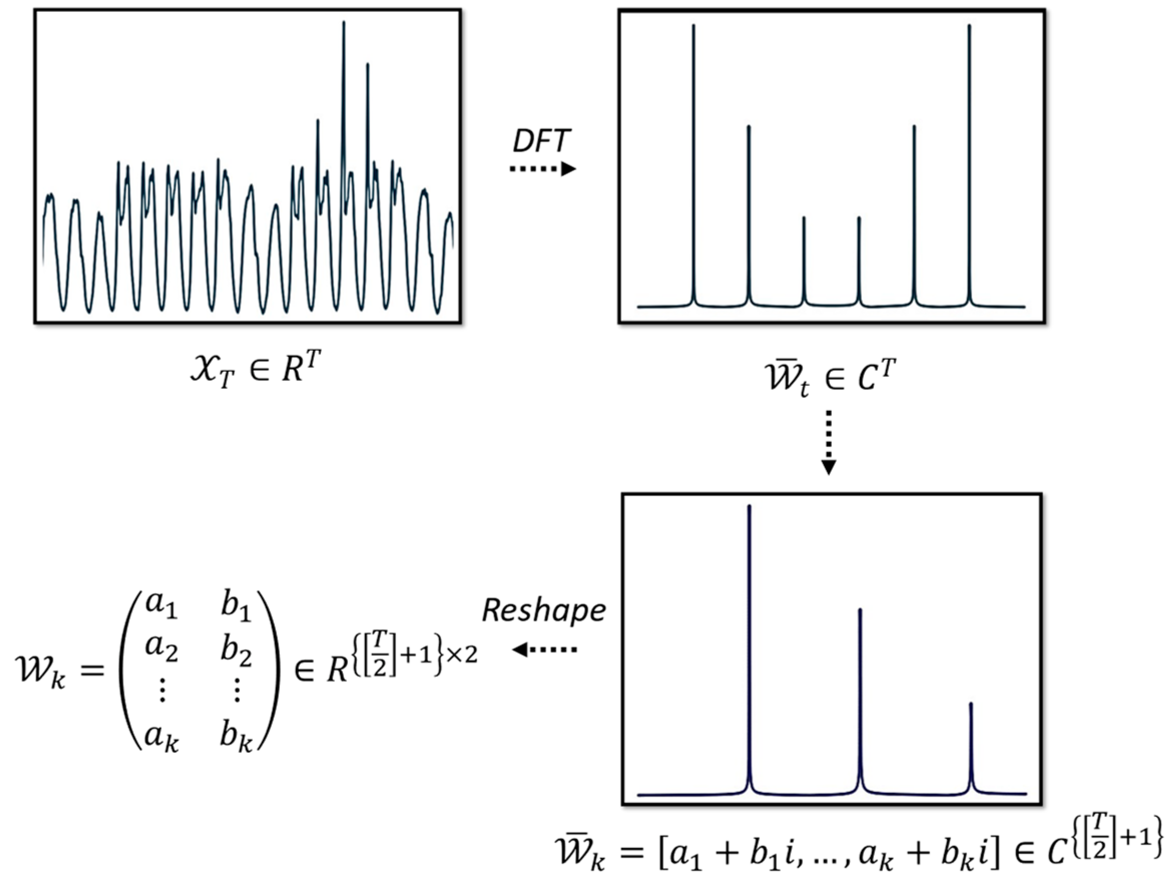
Figure 1. Preprocessing method, where i is imaginary unit.
Applsci 12 11912 g001
Figure 2. Multiscale convolutional layers.
Applsci 12 11912 g002
Figure 3. Multiscale backcast convolution neural network structure.
Applsci 12 11912 g003
Figure 4. Part of the Traffic dataset used in our experiments.
Applsci 12 11912 g004
Figure 5. Part of the test set prediction results for sensors 100~500. The curves are the prediction results of each sensor. The “Input”, “GT”, and “Prediction” below each curve correspond to the frequency domain representation of the input time series, the ground truth series, and the model prediction result. The core frequency components are accurately captured by our model, especially the low-frequency components with large amplitude.
Applsci 12 11912 g005
Table 1. Training Hyperparameter Configuration.
HyperparameterValue
Batch Size128
Epoch40
Early Stop3
Learning Rate (Initial value)0.0005
Input Timestamp Length96
Prediction Length96
Model Hidden Dimension512
Table 2. Comparison of Results Different Models.
ModelMSEMAECORR
Ours0.62720.36290.8592
Autoformer [19]0.65210.39830.8212
StemGNN [18]0.73840.46220.7971
LSTM 0.66520.37210.8579
Table 3. Results of Ablation Experiments.
ModelMSEMAECORR
MBCNN0.62720.36290.8592
none-backcast0.63980.37220.8542
none-dilation0.63760.37630.8537
none-dilation-backcast0.64610.37810.8511
Publisher’s Note: MDPI stays neutral with regard to jurisdictional claims in published maps and institutional affiliations.