Article

Evaluation of Different Control Algorithms for Carbon Dioxide Removal with Membrane Oxygenators

1
Institute of Engineering Design and Product Development, TU Wien, 1060 Vienna, Austria
2
Institute of Chemical, Environmental and Bioscience Engineering, TU Wien, 1060 Vienna, Austria
*
Author to whom correspondence should be addressed.
Appl. Sci. 2022, 12(23), 11890; https://doi.org/10.3390/app122311890
Submission received: 20 September 2022 / Revised: 18 November 2022 / Accepted: 18 November 2022 / Published: 22 November 2022
(This article belongs to the Special Issue Control Systems Approaches and Applications for Biomedical Systems)

Abstract

:
Membrane oxygenators are devices that benefit from automatic control. This is especially true for implantable membrane oxygenators—a class of wearable rehabilitation devices that show high potential for fast recovery after lung injury. We present a performance comparison for reference tracking of carbon dioxide partial pressure between three control algorithms—a classical proportional-integral (PI) controller, a modern non-linear model predictive controller, and a novel deep reinforcement learning controller. The results are based on simulation studies of an improved compartmental model of a membrane oxygenator. The compartmental model of the oxygenator was improved by decoupling the oxygen kinetics from the system and only using the oxygen saturation as an input to the model. Both the gas flow rate and blood flow rate were used as the manipulated variable of the controllers. All three controllers were able to track references satisfactorily, based on several performance metrics. The PI controller had the fastest response, with an average rise time and settling time of 1.18 s and 2.24 s and the lowest root mean squared error of 1.06 mmHg. The NMPC controller showed the lowest steady state error of 0.17 mmHg and reached the reference signal with less than 2% error in 90% of the cases within 15 s. The PI and RL reached the reference with less than 2% error in 84% and 50% of the cases, respectively, and showed a steady state error of 0.29 mmHg and 0.5 mmHg.

1. Introduction

Blood membrane oxygenators are devices that are widely used in extracorporeal circuits taking over the function of the lungs during surgical procedures [1]. Alternatively, they can be used to assist respiration and decrease the load on a lung under mechanical ventilation [2]. A miniaturized implantable membrane oxygenator could complement the physiological ventilation and help the lungs rehabilitate after a lung injury or a lung disease [3].
There are two main modes of operation of a membrane oxygenator. It can either be used to deliver enough oxygen to the blood or to remove carbon dioxide from the blood. The difference lies in the transport efficiency mismatch between the two gases. CO2 content in blood (approximately 0.5 mL/mL at 37 °C and 750 mmHg) significantly exceeds that of O2 (approximately 0.2 mL/mL at 37 °C and 750 mmHg). While O2 is mainly bound to hemoglobin, CO2 is mainly bound in blood in the form of bicarbonate. The different binding of the two gases influences the control strategy and the operating conditions—blood flow rate, sweep gas flow rate, and sweep gas partial pressure, depending on the operation mode. Generally, the oxygenation mode needs higher blood flow rates than the CO2 removal mode [4].
State-of-the-art membrane oxygenators consist of a packing of cylindrical hollow and asymmetric polymethylpentene fibers that are usually arranged concentrically along the long axis of the device. The blood flows on the shell side of the membrane fibers and is pumped by a blood pump, while the sweep gas is pumped through the lumen side of the membranes. The gas phase and the blood phase exchange CO2 and O2 through the permeable membrane, due to the partial pressure differences of the gases in both phases. The sweep gas usually consists of O2 and N2 in different ratios, while the CO2 concentration should be close to zero, in order to maximize partial pressure differences. Thus, CO2 diffuses from the blood into the sweep fluid and gets removed to the ambient, while O2 diffuses through the membrane into the blood. For a detailed review of membrane oxygenators, the interested reader is referred to [5].
In the clinics, the heart–lung machine (oxygenator, blood pump, and all periphery) is controlled by a perfusionist. The perfusionist is a highly trained member of the medical staff whose role [6], among others, is to adjust the parameters of the blood oxygenator—blood flow rate, gas flow rate, and sweep oxygen—content in a way that sets the CO2 partial pressure and blood oxygenation at desired levels [7]. Due to the human factor, this process is prone to errors that can lead to serious injuries to tissues and organs [8]. An automatic controller with accurate reference tracking can reduce the costs and treatment risks. For future wearable intracorporal membrane oxygenators, automatic control is obligatory, since a perfusionist is not available outside a clinical setting. Therefore, here we present a feasible method to automatically control these classes of devices.
Many efforts can be found in the literature that attempt to automate the heart–lung machine. Most of the works focus on controlling blood oxygenation with proportional-integral (PI) controllers, but some also take care of CO2 removal. Misgeld et al. [9] developed a PI controller with gain scheduling for the control of both blood gases. Manap et al. recently proposed a self-tuning fuzzy-PI [10] that follows setpoints for the CO2 partial pressure in the blood. Sadati et al. [11] proposed a fractional PI that controls the oxygen partial pressure. Allen et al. [12] presented a linear quadratic gaussian controller to control the oxygenation of the blood. All of the above-mentioned studies used the sweep flow rate as the manipulated variable.
In this work, we compare three different control algorithms for reference tracking of the CO2 partial pressure in a membrane oxygenator using both the sweep flow rate and blood flow rate as manipulated variables. To that end, first, a compartmental model of the blood membrane oxygenator is presented, detailing the CO2 kinetic and transport. Next, the three control algorithms are introduced—a PI feedback controller, a non-linear model predictive controller (NMPC), and a deep reinforcement learning (RL) controller. Their effectiveness in tracking setpoints and rejecting disturbances is presented. Finally, based on the results of the experiments, the advantages and disadvantages of each control algorithm are discussed.

2. Modeling and Control

2.1. Mathematical Model

The model of the membrane oxygenator (Appendix A Table A1) has been adopted from a compartmental model of the lungs described by Hill et al. [13]. The compartmental model is suitable for simulations for control applications because it is inexpensive to simulate, compared to models that calculate the spatial distribution of variables [14]. The compartments are assumed to be homogenous at all times, i.e., the perfect mixing of the compartments. The three compartments are gas, blood plasma, and erythrocytes (Figure 1a). These compartments exchange carbon dioxide in different forms: dissolved, bound to proteins, or converted to bicarbonate. The whole model consists of nine differential equations describing the dynamics of the three compartments.

2.1.1. Gas Compartment

In the membrane oxygenator, the dissolved CO2 from the blood diffuses through the membrane into the gas phase and gets removed from the system with the sweep gas flow.

2.1.2. Plasma Compartment

In the plasma compartment, CO2 exists in its dissolved form and as a bicarbonate. Here, the CO2 gets hydrated to carbonic acid, which then dissociates to bicarbonate and hydrogen ions. The plasma compartment exchanges dissolved CO2 with the gas compartment of the oxygenator and CO2 and HCO3 with the erythrocytes.

2.1.3. Erythrocytes Compartment

In the erythrocytes, CO2 exists in all three forms—dissolved, bound to proteins, and as a bicarbonate. Here, the hydration of CO2 is catalyzed by the enzyme carbonic anhydrase, which increases the reaction rate by a factor of ~104. Thus, when the partial pressure of CO2 ( p C O 2 , p l ) is high, CO2 would diffuse in the erythrocytes from the plasma, where it gets hydrated to HCO3, which then diffuses back into the plasma compartment. However, this generates a charge imbalance, because H+ ions are accumulating in the erythrocytes, due to the dissociation of carbonic acid, leading to a decrease in pH. To compensate for that, chloride diffuses from the plasma into the red blood cells (Hamburger shift [15]). The CO2 can also bind to hemoglobin and form carbamate. One hemoglobin molecule can bind to up to four CO2 molecules. The CO2 competes with O2 to bind to hemoglobin through the Bohr and Haldane effects. The Bohr effect describes the decreasing O2 affinity of hemoglobin at lower pH, thus improving O2 release under venous conditions. The Haldane effect refers to the reduced CO2 affinity of oxygen-saturated hemoglobin, which allows for improved CO2 release in the lungs.

2.1.4. Model Adjustment

Our model is adopted from the work of Hill et al. [13]. Others have previously [9,16,17,18] attempted similar adoptions. However, in [9,16,17], the dependence of S on the virtual pH and CO2 partial pressure is not considered when computing the rate of change of O2 concentration. They define the O2 concentration as:
[ O 2 ] b = α O 2 · p O 2 , b + c a p b · S ( p O 2 , v i r t u a l )
with
p O 2 , v i r t u a l = p O 2 , b · 10 0.024 ( 37 T ) + 0.4 ( pH v i r t u a l 7.4 ) + 0.06 × log 40 p CO 2
The rate of change of the O2 partial pressure is:
V b ( α O 2 + c a p b d S d p O 2 , v i r t u a l d p O 2 , v i r t u a l d p O 2 , b ) d p O 2 , b d t = Q b ( [ O 2 ] b , i n [ O 2 ] b ) + D O 2 , m V m , O 2 ( p O 2 , g p O 2 , b )
To acquire the rate of change of the O2 concentration, Equation (1) must be differentiated by time. However, in addition to p O 2 , b , pH v i r t u a l and p CO 2 , p l are also functions of time that are included in the system of differential equations (Appendix A Table A1). Therefore, the chain rule of differentiation requires Equation (2) to be differentiated, with respect to pH v i r t u a l and p CO 2 , p l , in addition to p O 2 , b , leading to:
V b d [ O 2 ] b d t = V b ( α O 2 d p O 2 , b d t + c a p b d S d p O 2 , v i r t u a l ( d p O 2 , v i r t u a l d p O 2 , b d p O 2 , b d t + d p O 2 , v i r t u a l d pH v i r t u a l d pH v i r t u a l d t + d p O 2 , v i r t u a l d p CO 2 , p l d p CO 2 , p l d t ) )
The right side of Equation (4) and the left side of Equation (3) are not equal. Manap et al. 2017 approached this issue by excluding only the incorrect equation from their model, but did not provide an alternative model for the oxygen kinetics. We solved the issue by excluding all oxygen kinetics from the dynamical system. However, the CO2 kinetics were coupled with the O2 kinetics through the Bohr and Haldane effects. We modelled that through the oxygen saturation curve and implemented it as a measured disturbance in our system. This had the effect of greatly simplifying the dynamical system and making it much less non-linear, compared to solving correctly for d [ O 2 ] b d t (Equation (4)). If one is interested in also controlling the oxygen concentration in the blood, then another feedback control loop can be designed that takes care of that specifically. Additionally, in Hexamer et al. (2003), Misgeld (2007), and Manap et al. (2017), there was a missing conversion factor in the membrane diffusion term in the rate of change equations of p C O 2 , p l and [ O 2 ] b . The amount of CO2 and O2, respectively, diffusing through the membrane was measured in l s−1, while all other terms were written in mol s−1. Here, the molar volume ( V m , CO 2 in Equation (A2), Appendix A Table A1) of O2 (~25.7301 L/mol) and CO2 (25.6312 L/mol) at 37 was required to balance the equations.

2.1.5. Model Implementation

The mathematical model of the membrane oxygenator was implemented in MATLAB/Simulink as a set of differential equations with the SymbolicToolbox, which were then solved numerically at each simulation step with a modified Rosenbrock formula of order 2 [19]. The inputs of the model were the blood and gas flow rate. The output was the CO2 partial pressure in the plasma. The blood saturation S and its time derivative were implemented as measured disturbances. The diffusion capacity of the membrane oxygenator was calculated from steady-state conditions of experimental data from in vitro and in vivo measurements [20]. The gas and blood volumes were calculated from the geometry of the oxygenator. The values for the remaining model parameters were taken from the literature (Appendix A Table A2). The initial values for the model variables are listed in Appendix A, Table A3. The non-model symbols used in the text are listed in Appendix A, Table A4.

2.2. Control

There are different possibilities for control strategies [21] of the membrane oxygenator. One example would be the maximization of the CO2 flux through the membrane. Another objective could be to set the CO2 flux at the desired value. In this work, we investigated a strategy that sets the concentration of CO2 in the blood at the desired value. This strategy was applied with three different algorithms—a classic PI controller, a modern non-linear model predictive controller, and a deep neural network-based reinforcement learning controller. Each controller acts both on the blood flow rate and the gas flow rate and has access to all system states.

2.2.1. PI Controller

A PI controller (Figure 1c)) is a classical control scheme that utilizes feedback to calculate an error from the desired output and adjust the control action based on that error. Proportional, integral, and derivative terms with adjustable coefficients are summed up to acquire the new action. There are many ways to tune the coefficients of the PI controller. In this work, the coefficients of the PI controller were tuned by identifying a linear state-space representation of the system from simulation data and designing a robust controller for it. The tuning algorithm used the Zieger–Nichols second method [22] to estimate the coefficients of the PI with at least 10 dB gain and 100 degrees phase margins. PI controllers are powerful and flexible; however, they are not optimal, in general. The problem is that they do not use a model of the system, but only feedback error and constant coefficients, meaning that they are reactive, instead of proactive

2.2.2. Non-Linear Model Predictive Controller

The non-linear model predictive controller (Figure 1d)) [23] is a proactive control scheme that uses a non-linear model of the system of the form:
x + = f ( x , u )
The idea is to predict and optimize a finite horizon trajectory for the future inputs— u —and states— x —of the system. Given the inputs and the current state, the future of the system can be calculated with the state equations (Appendix A Table A1. Equations (A1)–(A10)). However, the optimal inputs that guide the system into the desired state are not known in advance and have to be optimized for. To do that, the NMPC minimizes a quadratic cost function in the inputs and outputs under specified constraints, i.e.,
min u ( 0 ) , , u ( N 1 ) J ( x , u ) = k = 1 N 1 l ( x u ( k ) , u ( k ) )
with
l ( x u ( k ) , u ( k ) ) = x u ( k ) 2 + λ u ( k ) 2
The quadratic cost function (Equation (7)) not only penalizes deviation from the desired states but also imposes a penalty on the control action. The penalty ratio is controlled by the parameter λ 0 . For λ < 1 , deviation from the desired state is penalized more than control action and vice versa for λ > 1 . For λ = 0 , there is no penalty on the control action. Penalization of the control action has two advantages. First, imposing constraints on the possible u values make a solution easier to find numerically. Second, over-actuation, i.e., high u values, is associated with high energy consumption and even violating the physical constraints of the actuators. The NMPC minimizes the cost function over a finite time horizon, which is often different for the prediction and control sequences. After acquiring the optimal control sequence over the control horizon, the first element is applied to the system, and the optimization is repeated for each time step.

2.2.3. Reinforcement Learning Controller

Reinforcement learning (RL) is a machine learning paradigm where an agent acts in an environment (Figure 1e)), which is often modeled as a Markov decision process, that gives rewards as feedback. There are many types of RL algorithms, depending on how the actions are selected or how the learning happens [24]. In this work, a modification of the deep deterministic policy gradient (DDPG) [25] algorithm was used—the twin delayed deep deterministic policy gradient algorithm (TD3) [26]. DDPG is a model-free, off-policy, online reinforcement learning algorithm that uses an actor-critic architecture aiming to learn a policy π that maximizes the expected future reward r . The actor and critic are represented by deep neural networks to approximate the policy and Q-value functions. The actor follows the policy to select and apply actions a t ~ π that transition the environment to new states s t + 1 . The critic estimates the long-term value of an action Q π and critiques the actor on its actions by updating its estimation of the optimal policy [27]. The value function essentially estimates, in the long-term, what states would be visited, what action will be taken, and what reward will be accumulated by the agent, following the current policy. The rewards are given by a reward function, which defines the goal of the agent and has to be tailored for the specific application. The agent actively interacts with the environment, in order to maximize its reward. The ( s t , a t , r t , s t + 1 ) (state-action-reward-next state) tuples are the basis for changing the policy. An action followed by a high reward should be preferred over an action followed by a low reward. The Q-value of a particular state is equal to the reward collected after choosing an action according to the policy, plus the Q-value of the state reached, i.e.,
Q μ ( s t , a t ) = E [ r t + γ Q μ ( s t + 1 , μ ( s t + 1 ) ) ]
Equation (8) is called the Bellman equation. Here, the policy π is deterministic and parametrized by the function μ —a deep neural network. γ is a discount factor, giving less weight to future rewards. The learning is achieved through the n-step temporal difference algorithm, which looks n steps ahead to estimate the total value of a state and is based on the Bellman equation [28], but instead of the Q-value function, a target Q-value function is used, which is updated slowly throughout the training process. The update step of the parameters of the target value function is:
θ Q τ θ Q + ( 1 τ ) θ Q
with τ 1 .
The objective of the policy function is to optimize the expected future rewards, i.e.,
J ( θ ) = E [ Q ( s , a ) | s = s t . a = μ ( s t ) ]
The policy update (Equation (7)) is achieved in the direction of the gradient of the Q-value function [27].
θ μ = 1 N i a Q ( s , a | θ Q ) θ μ μ ( s | θ μ )
The sum in Equation (11) is over a random mini-batch of previous experiences from an experience buffer. Again, a target policy function is used that slowly updates throughout the training process. The target functions are approximated by a deep neural network and with the same architecture as the actor and critic. The target functions increase the stability of the optimization process because the networks are not referring to themselves in the weight update step (Equations (8) and (11)). The additional modifications that TD3 introduces are that there are two critics, instead of one, used to update the target value function. Additionally, the policy is updated less frequently than the value function, and the target policy is regularized, such that similar actions bring similar rewards.
To learn new things about the environment, the actions of the agent during the training process are superposed by correlated noise generated by an Ornstein–Uhlenbeck process. At the beginning of the training, the noise has higher values, which promotes the exploration of the environment. As the training advances, the noise amplitude decays, which allows the agent to exploit the best-learned strategy and score high rewards.

2.2.4. Imitation Learning

Finding the correct policy that controls the system in the desired fashion is very challenging and computationally expensive [29]. To reduce the training time needed to find an optimal policy, the actor can be pre-trained to imitate an expert controller. In this work specifically, we used examples from the NMPC controlling the membrane oxygenator system to pre-train the reinforcement learning agent. To that end, data comprising different setpoints for the p C O 2 , p l and actions taken by the NMPC were generated. Then, the actor neural network was trained to replicate them.

2.2.5. Controller Implementation

The controllers were implemented in MATLAB/Simulink and were interacting with a copy of the same model of the oxygenator system. The PI takes, as an input, only the tracking error and outputs blood flow rate and gas flow rate, which are min-max saturated to meet design criteria.
The NMPC has access to the reference, all states of the model, and the measured disturbances. It outputs the optimal blood flow rate and gas flow rate. The constraints on the control action are natively implemented in the optimization algorithm, which ensures an optimal solution. The value of the equal concern for the relaxation of constraints (ECR) parameter was set to 20, meaning that violating the constraints is allowed if no solution to the optimization can be found. After tuning the controller, the weights on the manipulated variables, the manipulated variable’s rates, and the weight for the output variable were set to (0.1, 0.1), (1, 1), and 10, respectively. The NMPC had a control horizon of 2 samples and a prediction horizon of 10 samples. It is a good idea to ‘warm start’ the controller by passing the resulting sequences of the last optimization procedure as initialization of the current one because it facilitates finding a solution faster. The actual numerical minimization of the cost function was achieved with an algorithm based on the interior point method [30,31].
The reinforcement learning controller also had access to all states and measured disturbances, but also to the tracking error and the integrated tracking error, which helped with disturbance rejection [32]. The constraints on the control action were implemented in the definition of the actor. For each controller, both the blood flow rate and the gas flow rate were constrained between 60 mL/min and 1200 mL/min. The RL agent was trained for 15,000 episodes, where each episode consisted of 40 s of simulated time with a constant p C O 2 . p l setpoint (different for each episode) and changing saturation.
The actor networks were represented by an input and normalization layer, followed by three fully connected hidden layers with 64, 32, and 16 nodes, respectively. The fully connected layers had a rectified linear unit (ReLU) non-linear activation function. The output blocks of the network comprised an action layer with two nodes for each action, combined with a hyperbolic tangent non-linear activation function and, finally, a scaling output layer.
The critic networks had state and action input paths and a common path. The state input path consisted of a normalization input layer, followed by three fully connected hidden layers with 64, 32, and 32 nodes, respectively. The fully connected layers had a ReLU non-linear activation function. The action path consisted, again, of an input normalization layer and two fully connected hidden layers, with 64 and 32 nodes with a ReLU function. Both the state path and action path were fed into the common path, which had three fully connected hidden layers with 16 nodes with ReLU. The output layers of the network comprise a fully connected layer with eight nodes and the final layer which output the estimated value—a scalar.
The learning rate for the actor network was set to 0.001 and for the critic at 0.0001. The standard deviation of the Ornstein–Uhlenbeck process used for exploration started at 5% of the action range and decayed to 0.5% of the action range. The critic learned with the five-step temporal difference algorithm.

2.3. Control Experiments

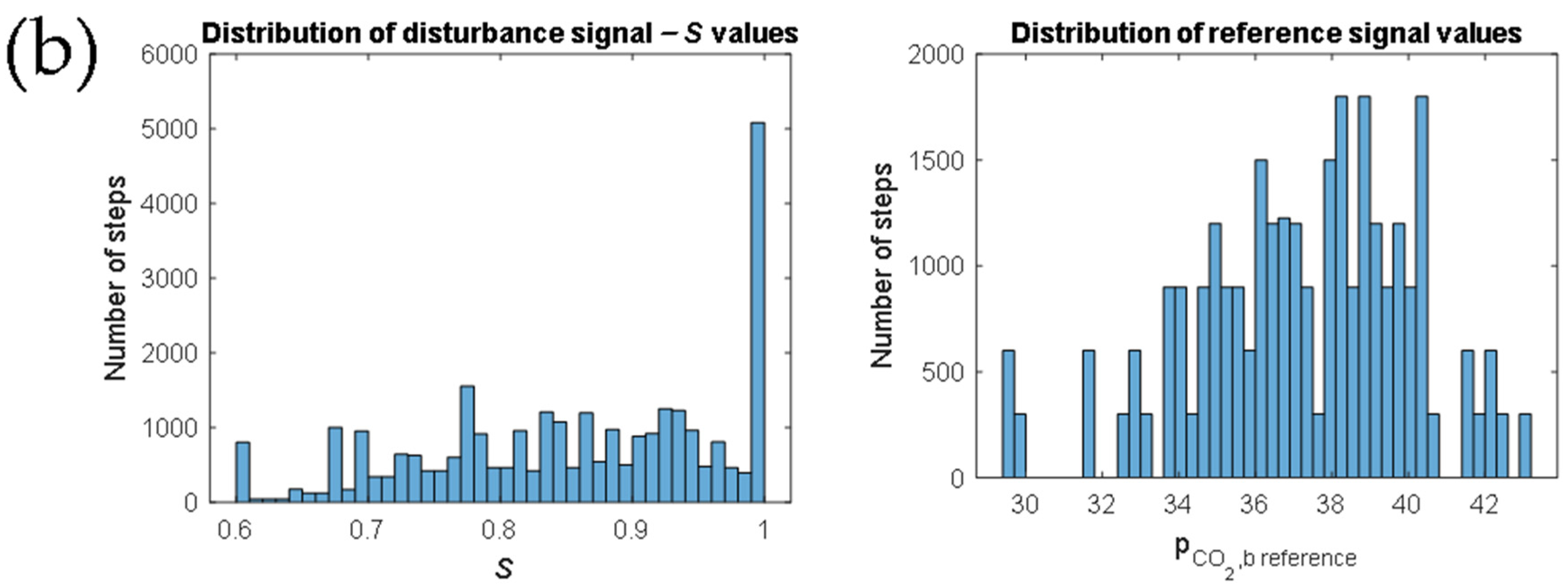
To assess the ability of the controllers to track reference signals, they were tested with a reference signal consisting of 100 step changes and a changing disturbance signal (Figure 2b). The whole experiment lasted 1500 s, or 100 step-like changes with a duration of 15 s each and 50 ramp-like changes in the disturbance signal with a duration of 30 s each. The reference signal had a mean of 37 mmHg and a standard deviation of 1.73 mmHg. The blood oxygen saturation disturbance signal had a mean of 85% and a standard deviation of 2.24%. The slope of the ramp was 0.25%/s. When a new target saturation was generated each 30 s, the ramp would continuously approach this target until it reached it, until the 30 s time ran out, or until one of the saturation limits was reached—minimum 60% and maximum 100% oxygen saturation. The performance of the controllers was assessed based on various relevant characteristics, as follows:

2.3.1. Rise Time

Rise time (RT) is defined as the time needed for the signal to rise from 10% to 90% of the magnitude of the step. It indicates how fast a controller reacts to setpoint change.

2.3.2. Settling Time

Settling time (ST) is the first time the error between the reference and the manipulated variable is less than 2% of the peak error. It indicates how fast a controller reaches a steady state.

2.3.3. Root-Mean-Squared Error

Root mean squared error (RMSE) is the square root of the average squared error between the setpoint and the signal. It indicates how closely setpoints can be tracked.

2.3.4. Action Power

The power of a signal is proportional to the integral of the signal squared. This characteristic shows the power expended by the motor for tracking references.

2.3.5. Action Standard Deviation

The standard deviation σ of the actions produced by the controllers was calculated. This characteristic was used as a proxy for patient comfort. The more varying the signals, the more perceived noise the device would make. Additionally, high variations in Q b might be unpleasant for the patient.

3. Results and Discussion

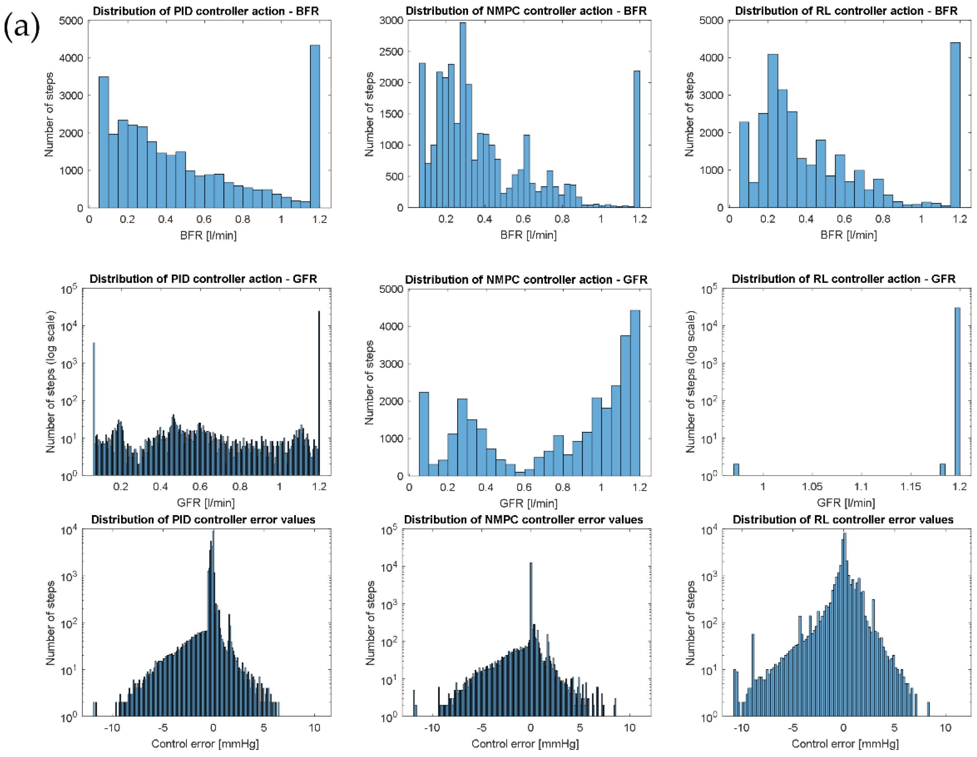
All controllers were able to track the reference signal accurately, while rejecting the disturbance acting on the system. Figure 3 shows a 250 s long snip from the experiment. The PI and NMPC signals had a very similar appearance, which was also confirmed by the measured signal characteristics in Table 1. The steady state error of the PI was larger than the NMPC; however, the NMPC showed an action delay of around five samples, or 25 ms, as can be seen in Figure 3. This action delay could explain the higher RMSE of the NMPC, compared to the PI, even though its steady state error was generally lower—0.17 mmHg vs. 0.29 mmHg. The RL controller had the highest steady state error at 0.5 mmHg, and the high rise and settling time increased its overall RMSE further. Additionally, often the RL controller did not even reach the reference, with less than 2% error in 50% of the cases in the given 15 s window. In comparison, the PI did not reach the reference in 16% and the NMPC in only 10% of the cases. From Figure 3, it can also be seen that the blood flow rate signal of the PI showed the highest spectral density, compared with RL and NMPC. The gas flow rate signal for NMPC had the highest spectral density, while for RL, it was almost constant. More than 99.993% of the sweep flow rate values of RL were at the maximum of the range (Figure 2). PI also showed quite polarizing values for the gas flow rate. Around 70% of all gas flow rates were either the maximum or the minimum of the range. Even though the NMPC controller also tended towards maximum gas flow rate values, its actions were more evenly distributed than RL and PI. The reference tracking error of the NMPC had a mean of −0.12 mmHg and a standard deviation of 1.09 mmHg. The PI error had a mean value of −0.29 mmHg and a standard deviation of 1.03 mmHg. The RL error had a 1.37 mmHg standard deviation with a 0 mean.
Table 1 summarizes the results of the measured characteristics during the experiments. The PI showed the lowest RT at 1.18 s, the lowest RMSE at 1.06 mmHg, and the lowest ST at 2.24 s. However, the PI also showed the most variance in its actions, while the RL produced the most stable inputs for the gas flow rate. For the blood flow rate, the NMPC produced the least varying actions. The NMPC showed the least power consumption for both the blood and gas flow rates, while RL showed the most for gas flow rate and PI for blood flow rate.
In the context of cardiopulmonary bypass and blood oxygenation, the gas flow rate was the main manipulated variable because the system usually takes over the whole blood circulation and oxygen requirement. There were strict constraints on the values that the blood flow rate can take, so that physiological conditions were maintained, and there was minimal clotting in the oxygenator [4]. However, for carbon dioxide removal systems, the blood flow rate seemed to be more appropriate. The plasma carbon dioxide partial pressure was much more sensitive to the blood flow rate, compared to the sweep flow rate—602.7 mmHg L−1 s−1 for blood and 363.2 mmHg L−1 s−1 for gas flow rate in the range of 0 to 1.2 L/min. Since the systemic circulation was usually intact, in the carbon dioxide removal context, the blood flow rate through the catheter could be freely regulated to achieve the desired conditions. Under this assumption, the RL controller optimized to a state in which it omitted the gas flow rate for the control of the CO2 partial pressure, setting it to an almost constant value.
When the control action was not constrained with a lower bound, all controllers simply set the desired CO2 concentration and then switched off all action. This was not the desired behavior because the CO2 flux, in this case, became 0. The literature refers to this behavior as reward hacking, which commonly arises in reinforcement learning tasks [33]. Interestingly, not only the RL but also the PI and the NMPC controllers found this to be an optimal solution to the task. The goal of PI and NMPC controllers is to set p C O 2 , p l with as little deviation as possible from the reference. Blood coming into the oxygenator from the body circulation has almost always different p C O 2 then the one in the oxygenator, because the gas gradients in the oxygenator are opposite to the ones in the body. Thus, the incoming blood counteracts the efforts of the controller to set the p C O 2 , p l at the reference value. It is, therefore, beneficial for the controller to turn off this ‘disturbance’, which leads to this undesired behavior. We solved this issue by implementing a low limit of 60 mL/min for the flow rates that counteract this behavior. The upper limit of 1.2 L/min was chosen, with regard to physiology, equipment limits, and the sensitivity curve of the p C O 2 p l , . Applying these saturation limits after the controller output was the only way to solve this problem for the PI. NMPC allows the constraints to be implemented in the optimization, which makes its solution optimal. However, this issue could also be solved by including a CO2 flux term in the cost function of the NMPC. On the other hand, the RL controller does not always converge to this sub-optimal solution. Our data indicate that the stochasticity in the exploration strategy of the RL agent could be the cause for this behavior.
While compared to the NMPC, the RL and PI controllers showed inferior accuracy in the reference tracking and disturbance rejection task, and they need much fewer computation resources to work, which might be a decisive factor if the optimization of the NMPC does not allow for online use. The tuned NMPC needed, on average, 0.13 s to optimize for an action, which was less than its sample time of 0.4 s, and can, thus, be implemented for online use. However, we found NMPC controllers with different weights that needed, on average, up to 0.63 s to optimize for a control step. This problem arose from the time complexity of the interior point method, which was hard to determine and was dependent, among others, on the weights of the controller and on the quality of the starting point [34]. In comparison, the time complexity of the RL agent actions was ~ O ( k 1 n × m ) , with m—the number of neurons for the current layer of the actor network, n-the number of neurons of the next layer, and k was the number of layers. On average, the RL agent needed 7.24 × 10⁻⁴ s to compute an action. The time complexity of the PI algorithm was ~ O ( p ) , where p was the number of outputs. The average time needed to compute an action of the PI controller was 6.69 × 10⁻⁷ s. There was a performance advantage of ~3 orders of magnitudes between PI and RL and RL and NMPC, when it came to computation time. Regarding memory requirements, PI needs 6 coefficients and takes about 1 kB of memory, NMPC needs around 30 coefficients and takes about 10 kB of memory, while the RL algorithm uses around 1.2 × 10⁻⁴ coefficients and takes around 300 kB of memory. Additionally, the PI controller is a very well-understood off-the-shelf algorithm that is very easy to implement, while the NMPC is a much more complicated control scheme that also needs an accurate model of the system, which might also imply the need for domain knowledge. On the other hand, RL is a model-free algorithm and, thus, does not need any domain knowledge. Training of the neural networks takes a long time, but after the agent is deployed, the selection of actions is fast and computationally inexpensive. The biggest disadvantage of the PI is the noisy nature of its actions. During operation, the high variability in Q b and Q g could lead to patient discomfort, or even potential harm [8,35]. This is not the case with NMPC, because it penalizes varying inputs in its cost function.
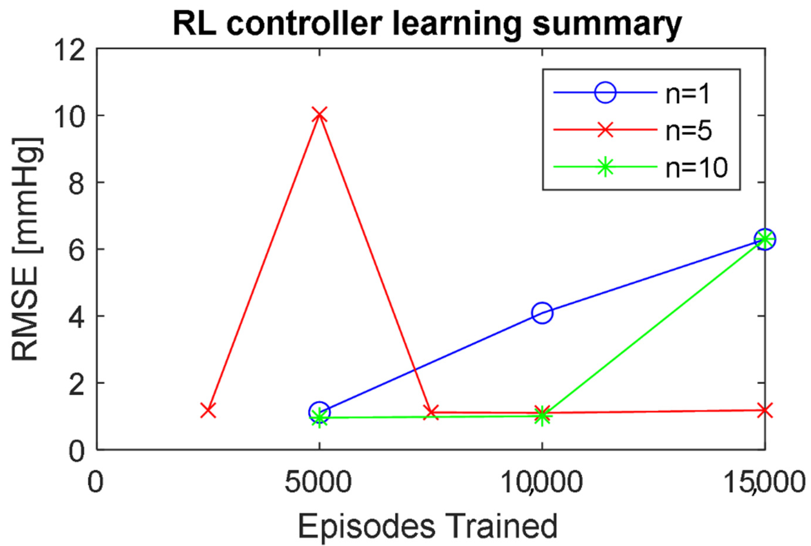
In order to investigate the effect on the policy divergence of n—the steps to look ahead for the n-step temporal difference algorithm, three agents with n = 1, 5, and 10 were trained for 15,000 (6 million steps) episodes on the membrane oxygenator model. The trained controllers were tested on a reference tracking task consisting of 50 random step-like setpoint changes (with the same random seed for comparison), and the RMSE between the setpoint and the actual p C O 2 , p l was calculated. Figure 4 shows the results. The agents with n = 1 and 10 showed diverging behavior with increased training. After the full 15,000 episodes, both controllers kept constant blood and gas flow rates, without attempting to track the reference signal. Divergence often occurs when the critic learns unfeasibly large values for state-action pairs and then, based on those critiques, the actions of the actor, thus changing its policy [36]. On the other hand, the agent with n = 5 remained stable after 15,000 episodes, even though its RMSE slightly increased from its minimum at 10,000 episodes—from 1.1 mmHg to 1.18 mmHg. There was a huge increase in the RMSE for n = 5 at 5000 episodes. This agent gave up and set the blood flow rate at the minimum value for the rest of the experiment after trying for several steps to track the highest setpoint in the validation set of 42.4 mmHg. This, again, can be explained as a mistake by the critic, who probably estimated more value in switching off the control action (which is penalized slightly by the reward function), instead of trying to track this untrackable reference. This, however, is unacceptable behavior, which illustrates the issues of black box control methods for medical devices.

4. Conclusions

This work presents a comparison between PI, NMPC, and deep RL control algorithms for blood CO2 partial pressure reference tracking for membrane oxygenators in simulation. While PI and RL require less computational power when deployed, the NMPC was found to be the most suitable overall, in terms of accuracy, speed, and patient comfort. However, hardware limitations could restrict the use of an NMPC controller.
Furthermore, a compartmental dynamical model of a membrane oxygenator was presented, which fixed and simplified the already existing model, without a loss of information for the carbon dioxide removal setting.
Additionally, it was shown that the blood flow rate was suitable to be a manipulated variable in the carbon dioxide removal setting of membrane oxygenators. All three types of controllers used both the sweep and the blood flow rate to achieve reference tracking and disturbance rejection.
The oxygenator model that was used for the assessment of the performance of the different control algorithms has several limitations. Firstly, it is assumed that the compartments are perfectly mixed, i.e., are homogenous. This means that the concentration polarization layer effect at the membrane surface is not considered, which can negatively affect the gas flux through the membrane. However, this simplification is necessary because solving for the spatial concentrations is very computationally expensive and is not suitable for the presented application. Furthermore, most of the parameters of the model are temperature-dependent, while in the presented model, the values for 37 °C are used. This issue can be fixed by including the temperature as an additional disturbance acting on the model and modeling the temperature dependence of the variables. Finally, changing the blood flow rate also changed the pressure inside the catheter, which could lead to potential harm to the patient. However, because our catheter allows the blood to flow also around it in the vena cava and the drainage and return sites are close to each other, changing the blood flow rate should not induce high pressure changes in the circulation system of the patient. Recirculation, which is usually an undesired phenomenon because it lowers the efficiency of the system to exchange gases, helps in this case to keep blood pressure within physiological conditions. Further investigations should be carried out to test this hypothesis.
In the previous work, we presented an accurate estimator for the most important hydrodynamic parameters of the blood—flow rate, pressure difference, and viscosity [37]. Together with the control of the gases, the most important vital parameters—hemodynamics and gas exchange—were covered. In future work, they have to be integrated into one control system and their performance investigated and validated in in silico, in vitro, and then, finally, in vivo settings.
Membrane oxygenators are medical devices, thus patient safety is one of the main concerns. Any automatic control scheme has to show proof of robustness and stability before it can be applied to any human patient. Additionally, safety control mechanisms can be implemented to supplement the control of hemodynamics and blood gases. A venous–venous membrane oxygenator can benefit from a pressure detection system that can be used for suction prevention and thrombus detection. Moreover, the blood flow rate control can be extended to pulsatile control to mimic better physiological conditions.

Author Contributions

Conceptualization, M.E., B.L., P.E. and C.J.; methodology, M.E.; software, M.E.; validation, M.E., B.L., P.E. and C.J.; formal analysis, M.E.; investigation, M.E.; resources, M.G. and M.H.; writing—original draft preparation, M.E.; writing—review and editing, M.E., B.L., P.E., C.J. and M.G.; visualization, M.E; supervision, M.G.; project administration, M.G.; funding acquisition, M.G. and M.H. All authors have read and agreed to the published version of the manuscript.

Funding

This research was partially funded by the Austrian Research Promotion Agency (FFG). Project: MILL—Minimally Invasive Liquid Lung, grant number 857859.

Institutional Review Board Statement

Not applicable.

Informed Consent Statement

Not applicable.

Conflicts of Interest

The authors declare no conflict of interest.

Appendix A

Table A1. Model equations for the compartmental model.
Gas compartment
V g d p CO 2 , g d t = Q g ( p CO 2 , g , i n p CO 2 , g ) + D CO 2 , m × p b a r ( p CO 2 , p l p CO 2 , g ) (A1)
Plasma compartment
V p l α CO 2 d p CO 2 , p l d t = Q p l α CO 2 ( p CO 2 , p l , i n p CO 2 , p l ) + D CO 2 , m V m , CO 2 ( p CO 2 , g p CO 2 , p l ) + D CO 2 , r b c ( p CO 2 , r b c p CO 2 , p l ) + V p l R HCO 3 , p l (A2)
V p l d [ HCO 3 ] p l d t = Q p l ( [ HCO 3 ] p l , i n [ HCO 3 ] p l ) D HCO 3 , r b c ( [ HCO 3 ] p l [ HCO 3 ] r b c r ) V p l R HCO 3 , p l (A3)
V p l d [ H ] p l d t = Q p l ( [ H ] p l , i n [ H ] p l ) V p l 2.303 β p l [ H ] p l R HCO 3 , p l (A4)
R HCO 3 , p l = k u α C O 2 p CO 2 , p l + k v k [ H ] p l [ HCO 3 ] p l (A5)
Erythrocytes compartment
V r b c α CO 2 d p CO 2 , r b c d t = Q r b c α CO 2 ( p CO 2 , r b c , i n p CO 2 , r b c ) D CO 2 , r b c ( p CO 2 , r b c p CO 2 , p l ) + V r b c R HCO 3 , r b c V r b c d carb d t (A6)
V r b c d [ HCO 3 ] r b c d t = Q r b c ( [ HCO 3 ] r b c , i n [ HCO 3 ] p l ) + D HCO 3 , r b c ( [ HCO 3 ] p l [ HCO 3 ] r b c r ) V r b c R HCO 3 , r b c (A7)
V r b c d [ H ] r b c d t = Q r b c ( [ H ] r b c , i n [ H ] r b c ) + V r b c 2.303 β r b c [ H ] r b c ( R HCO 3 , r b c + 1.5 d carb d t 0.6 d S d t ) (A8)
V r b c d [ carb ] d t = Q r b c ( [ carb ] i n [ carb ] ) + k a p CO 2 , r b c α CO 2 V r b c ( [ Hb ] [ carb ] ) ( k z o S k z o + [ H ] r b c + k z r ( 1 S ) k z r + [ H ] r b c ) V r b c k a [ carb ] [ H ] r b c k c (A9)
d pH v i r t u a l d t = 10 ( pH v i r t u a l lg ( r [ H ] r b c ) ) (A10)
R HCO 3 , r b c = c a t ( k u α C O 2 p CO 2 , r b c + k v k [ H ] r b c [ HCO 3 ] r b c ) (A11)
r = ( 0.058 × pH v i r t u a l 0.437 ) S 0.529 × pH v i r t u a l + 4.6 (A12)
Table A2. Summary of model parameters.
SymbolParameterValueUnit
V g Gas volume0.0055L
V b Blood volume0.0121L
V p l Plasma volume V b × ( 1 h c t ) L
V r b c Erythrocyte volume V b × h c t L
D CO 2 , m Membrane diffusion capacity5.4 × 10−6L (mmHg s)−1
p b a r Gas pressure760mmHg
α CO 2 CO2 solubility coefficient3.5 × 10−5M mmHg−1
V m , CO 2 CO2 molar volume25.64M−1
D CO 2 , r b c Erythrocyte diffusion capacity for CO2 0.693 α CO 2 τ r b c V p l V r b c V p l + V p l M L (mmHg s)−1
D HCO 3 , r b c Erythrocyte diffusion capacity for HCO3 0.693 α CO 2 τ H C O 3 V p l V r b c V p l + V p l M L (mmHg s)−1
τ r b c CO2 half-time erythrocyte membrane diffusion0.001s
τ H C O 3 HCO3 half-time erythrocyte membrane diffusion0.2s
β p l Buffer capacity plasma6 × 10−3M pH−1
β r b c Buffer capacity erythrocytes57.7 × 10−3M pH−1
k u CO2 hydration reaction forward constant0.12s−1
k v CO2 hydration reaction reverse constant89s−1
k Carbonic acid dissociation equilibrium constant5.5 × 10−4M
k a Carbamate generation forward constant5 × 103(M s)−1
k z o Oxygenated hemoglobin ionization constant8.4 × 10−9M
k z r De-oxygenated hemoglobin ionization constant7.2 × 10−8M
k c Carbamate ionization constant2.4 × 10−5-
c a t Carbonic anhydrase catalytic factor13,000-
[ Hb ] Hemoglobin concentration20.7 × 10−3M
Table A3. Summary of model variables. The initial values for states, actions, and values for model disturbances are shown.
SymbolVariableDescriptionUnitValue
p CO 2 , g Partial pressure CO2 gas oxygenatorstatemmHg0.695
p CO 2 , g , i n Partial pressure CO2 gas venousdisturbancemmHg0
p CO 2 , p l Partial pressure CO2 plasma oxygenatorstate, outputmmHg43
p CO 2 , p l , i n Partial pressure CO2 plasma venousdisturbancemmHg46
p CO 2 , r b c Partial pressure CO2 erythrocyte oxygenatorstatemmHg43.1
p CO 2 , r b c , i n Partial pressure CO2 erythrocyte venousdisturbancemmHg46
[ HCO 3 ] p l Bicarbonate concentration plasma oxygenatorstateM263 × 10−4
[ HCO 3 ] p l , i n Bicarbonate concentration plasma venousdisturbanceM263 × 10−4
[ HCO 3 ] r b c Bicarbonate concentration erythrocyte oxygenatorstateM183 × 10−4
[ HCO 3 ] r b c , i n Bicarbonate concentration erythrocyte venousdisturbanceM182 × 10−4
[ H ] p l Hydrogen concentration plasma oxygenatorstateM42.3 × 10−9
[ H ] p l , i n Hydrogen concentration plasma venousdisturbanceM42.3 × 10−9
[ H ] r b c Hydrogen concentration erythrocyte oxygenatorstateM61 × 10−9
[ H ] r b c , i n Hydrogen concentration erythrocyte venousdisturbanceM61 × 10−9
pH v i r t u a l Virtual pHstate-7.37
[ carb ] Carbamate concentrationstateM184 × 10−5
[ carb ] i n Carbamate concentration venousdisturbanceM235 × 10−5
S Blood oxygen saturationmeasured disturbance--
h c t Hematocritdisturbance-0.45
Q g Sweep gas flow ratemanipulated variableL/s-
Q b Blood flow ratemanipulated variableL/s-
Table A4. List of non-model symbols used in the text.
SymbolMeaning
CO2Carbon dioxide
O2Dioxygen
N2Dinitrogen
HCO3Bicarbonate Ion
HHydrogen
pHPotential of hydrogen
[ O 2 ] b Oxygen molar concentration
p O 2 , b Oxygen partial pressure
c a p b Blood oxygen capacity
p O 2 , v i r t u a l Virtual partial pressure of oxygen
T Temperature
α O 2 Oxygen solubility in blood
[ O 2 ] b , i n Venous oxygen molar concentration
D O 2 , m Membrane diffusion capacity for oxygen
V m , O 2 Oxygen molar volume
p O 2 , g Oxygen partial pressure in sweep gas
x + Future state vector
f ( x , u ) Function of x and u
x State vector
u Input vector
min Minimizing function
N Control horizon number of samples, number of transitions
J Cost
k Sample index
l Cost function
λ Regularization parameter
π Policy
Q Q-value function
t Time
a t Agent action at time t
s t Environment state at time t
r Reward
γ Future reward discount factor
μ Policy function
θ Function parameters (weights of the neural net)
Q Target Q-value function
τ Target function update rate

References

  1. Makdisi, G.; Wang, I.W. Extra Corporeal Membrane Oxygenation (ECMO) review of a lifesaving technology. J. Thorac. Dis. 2015, 7, E166–E176. [Google Scholar] [CrossRef] [PubMed] [Green Version]
  2. Jeffries, R.G.; Lund, L.; Frankowski, B.; Federspiel, W.J. An extracorporeal carbon dioxide removal (ECCO 2 R) device operating at hemodialysis blood flow rates. Intensive Care Med. Exp. 2017, 5, 41. [Google Scholar] [CrossRef] [Green Version]
  3. Kneyber, M.C. Mechanical ventilation during extra-corporeal membrane oxygenation: More questions than answers. Minerva Anestesiol. 2019, 85, 91–92. [Google Scholar] [CrossRef] [PubMed]
  4. Ficial, B.; Vasques, F.; Zhang, J.; Whebell, S.; Slattery, M.; Lamas, T.; Daly, K.; Camporota, N.A. Physiological basis of extracorporeal membrane oxygenation and extracorporeal carbon dioxide removal in respiratory failure. Membranes 2021, 11, 225. [Google Scholar] [CrossRef]
  5. Teber, O.O.; Altinay, A.D.; Mehrabani, S.A.N.; Tasdemir, R.S.; Zeytuncu, B.; Genceli, E.A.; Dulekgurgen, E.; Pekkan, K.; Koyuncu, İ. Polymeric hollow fiber membrane oxygenators as artificial lungs: A review. Biochem. Eng. J. 2022, 180, 108340. [Google Scholar] [CrossRef]
  6. Bouchez, S.; de Somer, F. The evolving role of the modern perfusionist: Insights from transesophageal echocardiography. Perfusion 2021, 36, 222–232. [Google Scholar] [CrossRef] [PubMed]
  7. Boeken, U.; Ensminger, S.; Assmann, A.; Schmid, C.; Werdan, G.; Michels, O.; Miera, F.; Schmidt, S.; Klotz, C.; Starck, K. Einsatz der extrakorporalen Zirkulation (ECLS/ECMO) bei Herz- und Kreislaufversagen. Kardiologe 2021, 15, 526–535. [Google Scholar] [CrossRef]
  8. Utley, J.R. Techniques for avoiding neurologic injury during adult cardiac surgery. J. Cardiothorac. Vasc. Anesth. 1996, 10, 38–44. [Google Scholar] [CrossRef]
  9. Misgeld, B.J.E.; Werner, J.; Hexamer, M. Simultaneous automatic control of oxygen and carbon dioxide blood gases during cardiopulmonary bypass. Artif. Organs 2010, 34, 503–512. [Google Scholar] [CrossRef]
  10. Manap, H.H.; Wahab, A.K.A.; Zuki, F.M. Control for Carbon Dioxide Exchange Process in a Membrane Oxygenator Using Online Self-Tuning Fuzzy-PID Controller. Biomed. Signal Process. Control. 2021, 64, 102300. [Google Scholar] [CrossRef]
  11. Sadati, S.J.; Noei, A.R.; Ghaderi, R. Fractional-order control of a nonlinear time-delay system: Case study in oxygen regulation in the heart-lung machine. J. Control Sci. Eng. 2012, 2012, 478346. [Google Scholar] [CrossRef] [Green Version]
  12. Allen, J.; Fisher, A.C.; Gaylor, J.D.S.; Razieh, A.R. Development of a digital adaptive control system for PO2 regulation in a membrane oxygenator. J. Biomed. Eng. 1992, 14, 404–411. [Google Scholar] [CrossRef]
  13. Hill, E.P.; Power, G.G.; Longo, L.D. A mathematical model of carbon dioxide transfer in the placenta and its interaction with oxygen. Am. J. Physiol. 1973, 224, 283–299. [Google Scholar] [CrossRef]
  14. Lukitsch, B.; Ecker, P.; Elenkov, M.; Janeczek, C.; Haddadi, B.; Jordan, C.; Krenn, C.; Ulrich, R.; Gfoehler, M.; Harasek, M. Computation of global and local mass transfer in hollow fiber membrane modules. Sustainability 2020, 12, 2207. [Google Scholar] [CrossRef] [Green Version]
  15. Klocke, R.A. Velocity of CO2 exchange in blood. Annu. Rev. Physiol. 1988, 50, 625–637. [Google Scholar] [CrossRef]
  16. Hexamer, M.; Werner, J. A mathematical model for the gas transfer in an oxygenator. IFAC Proc. Vol. 2003, 36, 409–414. [Google Scholar] [CrossRef]
  17. Misgeld, B.J.E. Automatic Control of the Heart-Lung Machine. Ph.D. Thesis, Ruhr-Universität Bochum, Universitätsbibliothek, Bochum, Germany, 2007. [Google Scholar]
  18. Manap, H.H.; Wahab, A.K.A.; Zuki, F.M. Mathematical Modelling of Carbon Dioxide Exchange in Hollow Fiber Membrane Oxygenator. IOP Conf. Ser. Mater. Sci. Eng. 2017, 210, 012003. [Google Scholar] [CrossRef]
  19. Shampine, L.F.; Reichelt, M.W. The MATLAB ODE Suite. SIAM J. Sci. Comput. 1997, 18, 1–22. [Google Scholar] [CrossRef] [Green Version]
  20. Lukitsch, B.; Ecker, P.; Elenkov, M.; Janeczek, C.; Jordan, C.; Krenn, C.G.; Ulrich, R.; Gfoehler, M.; Harasek, M. Suitable CO2 solubility models for determination of the CO2 removal performance of oxygenators. Bioengineering 2021, 8, 1–25. [Google Scholar] [CrossRef]
  21. Harasek, M.; Elenkov, M.; Lukitsch, B.; Ecker, P.; Janeczek, C.; Gfoehler, M. Design of Control Strategies for the CO2 Removal from Blood with an Intracorporeal Membrane Device. In Proceedings of the 11th Biomedical Engineering International Conference (BMEiCON), Chiang Mai, Thailand, 21–24 November 2018; pp. 1–4. [Google Scholar] [CrossRef]
  22. Ziegler, J.G.; Nichols, N.B. Optimum settings for automatic controllers. J. Dyn. Syst. Meas. Control. Trans. ASME 1993, 115, 220–222. [Google Scholar] [CrossRef] [Green Version]
  23. Grüne, L.; Pannek, J. Nonlinear Model Predictive Control Theory and Algorithms; Springer: Berlin/Heidelberg, Germany, 2017. [Google Scholar]
  24. Sutton, R.S.; Barto, A.G. Reinforcement Learning: An Introduction, 2nd ed.; The MIT Press: Cambridge, MA, USA, 2018. [Google Scholar]
  25. Lillicrap, T.P.; Hunt, J.J.; Pritzel, A.; Heess, N.; Erez, T.; Tassa, Y.; Silver, D.; Wierstra, D. Continuous control with deep reinforcement learning. arXiv 2015, arXiv:1509.02971. [Google Scholar] [CrossRef]
  26. Fujimoto, S.; van Hoof, H.; Meger, D. Addressing Function Approximation Error in Actor-Critic Methods. In Proceedings of the Proceedings of the 35th International Conference on Machine Learning, Stockholm, Sweden, 10–15 July 2015; Volume 4, pp. 2587–2601. [Google Scholar]
  27. François-lavet, V.; Henderson, P.; Islam, R.; Bellemare, M.G.; Pineau, J. An Introduction to Deep Reinforcement Learning. In Foundations and Trends® in Machine Learning; Mike Casey: University of California, Berkeley, CA, USA, 2018; Volume II, pp. 1–140. [Google Scholar] [CrossRef]
  28. Watkins, C.J.C.H.; Dayan, P. Q-learning. Mach. Learn. 1992, 8, 279–292. [Google Scholar] [CrossRef]
  29. Dulac-Arnold, G.; Mankowitz, D.; Hester, T. Challenges of Real-World Reinforcement Learning. arXiv 2019, arXiv:1904.12901. [Google Scholar]
  30. Byrd, R.H.; Gilbert, J.C.; Nocedal, J. A trust region method based on interior point techniques for nonlinear programming. Math. Program. Ser. B 2000, 89, 149–185. [Google Scholar] [CrossRef] [Green Version]
  31. Waltz, R.A.; Morales, J.L.; Nocedal, J.; Orban, D. An interior algorithm for nonlinear optimization that combines line search and trust region steps. Math. Program. 2006, 107, 391–408. [Google Scholar] [CrossRef]
  32. Rizvi, A.S.A.; Pertzborn, A.J.; Lin, Z. Reinforcement Learning Based Optimal Tracking Control Under Unmeasurable Disturbances with Application to HVAC Systems. IEEE Trans. Neural Netw. Learn. Syst. 2021, 1–11. [Google Scholar] [CrossRef]
  33. Amodei, D.; Olah, C.; Steinhardt, J.; Christiano, P.; Schulman, J.; Mané, D. Concrete Problems in AI Safety. arXiv 2016, arXiv:1606.06565. [Google Scholar]
  34. Potra, F.A.; Wright, S.J. Interior-point methods. J. Comput. Appl. Math. 2000, 124, 281–302. [Google Scholar] [CrossRef] [Green Version]
  35. Mills, N.L.; Ochsner, J.L. Massive air embolism during cardiopulmonary bypass. Causes, prevention, and management. J. Thorac. Cardiovasc. Surg. 1980, 80, 708–717. [Google Scholar] [CrossRef]
  36. Van Hasselt, H.; Doron, Y.; Strub, F.; Hessel, M.; Sonnerat, N.; Modayil, J. Deep Reinforcement Learning and the Deadly Triad. arXiv 2018, arXiv:1812.02648. [Google Scholar]
  37. Elenkov, M.; Lukitsch, B.; Ecker, P.; Janeczek, C.; Harasek, M.; Gföhler, M. Non-parametric dynamical estimation of blood flow rate, pressure difference and viscosity for a miniaturized blood pump. Int. J. Artif. Organs 2022, 45, 207–215. [Google Scholar] [CrossRef] [PubMed]
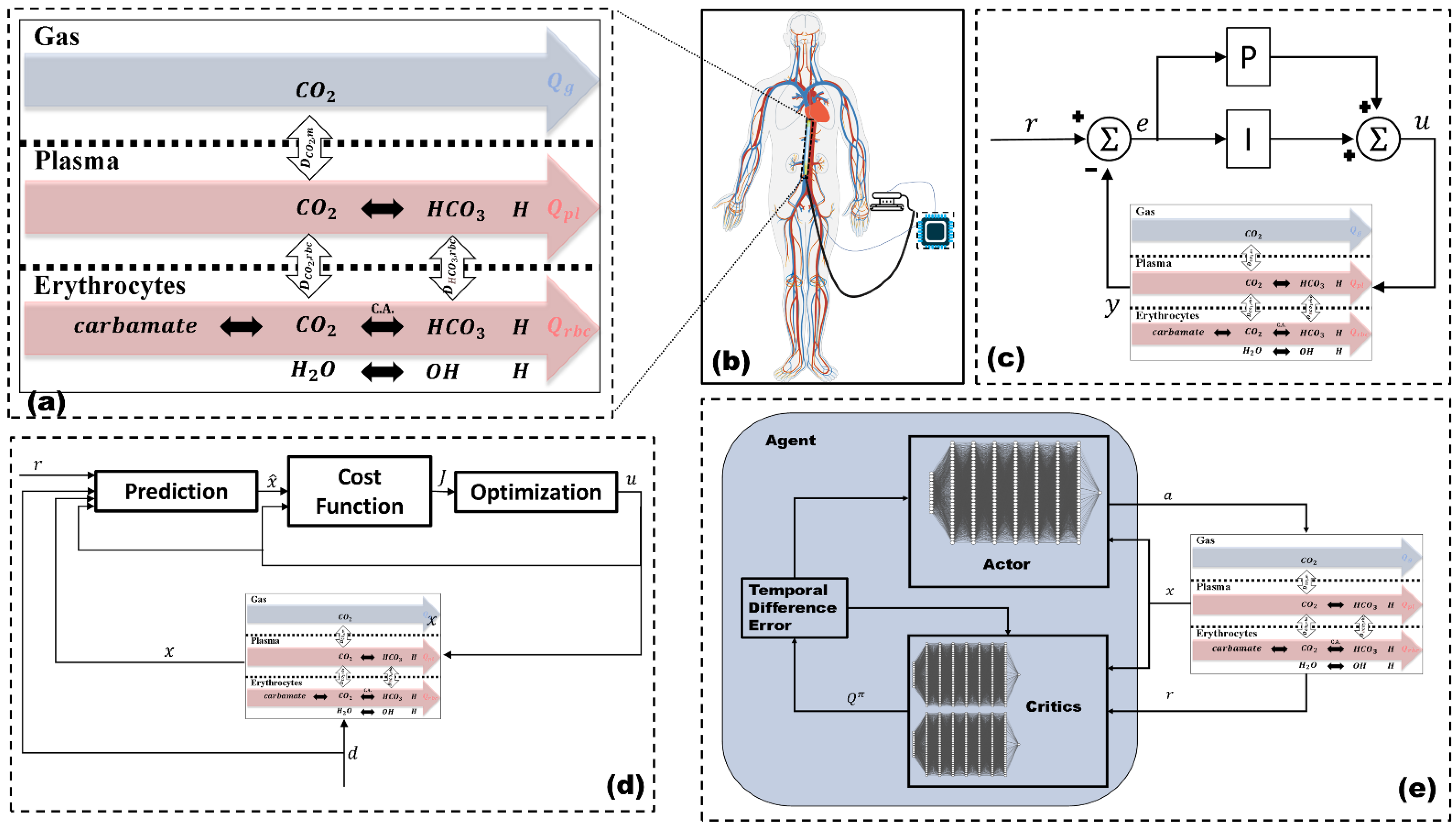
Figure 1. An overview of the system and controllers: (a) A schematic representation of the compartmental model of the membrane oxygenator; (b) A drawing of the physical system. The catheter—membrane oxygenator and blood pump—is inserted in the vena cava superior. The extracorporeal part of the device-controller and a compressor are worn by the patient; (c) A schematic representation of the PI controller; (d) A schematic representation of the NMPC controller; (e) A schematic representation of the deep RL controller.
Applsci 12 11890 g001
Figure 2. Statistics of the results of the experiments: (a) the distributions for the control action and reference tracking error for each controller; (b) distributions for the reference signal and the disturbance signal.
Applsci 12 11890 g002aApplsci 12 11890 g002b
Figure 3. Results of the control experiments. The top row shows setpoints and manipulated variable— p C O 2 , p l for the three controllers. The bottom row shows the actions taken—sweep flow rate (SFR) and blood flow rate (BFR)—by each controller for a snip of the reference tracking task. The disturbance S is also shown.
Applsci 12 11890 g003
Figure 4. Results of the RL controller training for n = 1, 5, and 10. The agents with n = 1 and 10 showed diverging behavior.
Applsci 12 11890 g004
Table 1. Results of the control experiments. The PI, NMPC, and RL controllers were assessed based on rise time (RT), settling time (ST), root-mean-squared error (RMSE), action power P, and action standard deviation σ.
PINMPCRL
RT [s]1.181.334.9
ST [s]2.243.577.6
RMSE [mmHg]1.061.091.37
P Q g [L2s−2]6.7 × 10−34.1 × 10−38 × 10−3
P Q b [L2s−2]2.2 × 10−31.4 ×10−32 × 10−3
σ Q g [mLs−1]6.536.530.03
σ Q b [mLs−1]6.35.055.95
Publisher’s Note: MDPI stays neutral with regard to jurisdictional claims in published maps and institutional affiliations.