Abstract
In this paper, two identification methods are proposed for a ground robotic system. A Gaussian process regression (GPR) model is presented and adopted for a system identification framework. Its performance and features were compared with a wavelet-based nonlinear autoregressive exogenous (NARX) model. Both algorithms were compared and experimentally validated for a small ground robot. Moreover, data were collected throughout the onboard sensors. The results show better prediction performance in the case of the GPR method, as an estimation algorithm and in providing a measure of uncertainty.
1. Introduction
Gaussian process regression (GPR) is a nonlinear modeling technique that has recently received interest in various fields of engineering. It provides a non-parametric and probabilistic model fully described by its mean and covariance functions. One of the advantages of the GP approach over traditional methods is its ability to provide information for the system even in off-equilibrium regions, where limited data are available. Moreover, with this method, the hyperparameters can be directly learned from the data points [1]. Furthermore, the analytic expression of the model uncertainty provided by GP models as well as the robustness against overfitting are useful for model-based control strategies.
GPs were first employed in the representation of the geostatistics field (also known as kriging) and then widespread in machine learning [2,3], robotics, controls, and system identification frameworks [4,5]. Models for various spatial and temporal problems, such as Brownian motion, Langevin processes, and Wiener processes are examples of GP applications [6]. A consistent number of publications can be found about the use of parametric prediction methods to obtain a mathematical model of a dynamic system from observed input–-output data. Considering classical approaches, such as prediction error methods (PEM), statistical properties of prediction error are used to build an optimal model by selecting a proper model structure, as in [7]. Linear structures, such as black box structures, include the FIR model (finite impulse response model), OE model (output error model), ARX model (autoregressive with an external input model), ARMAX model (autoregressive moving average with external input model), and BJ model (Box–-Jenkins model), but nonlinear black box modeling techniques are also available (see [8] for an overview). Some of the examples that can be found in the literature are neural networks, fuzzy logic-based models, and wavelet expansions. They is evidence of the influence of machine learning techniques in system identification fields. A survey of different techniques can be found in [9]. Furthermore, some research is focused on the non-convex optimization problem that provides the model parameters, and on methods to improve convergence to the optimal solution. In [10], the authors provide an overview on the use of evolutionary strategies and swarm algorithms in the field of system identification. In a more recent contribution [11], a novel fractional hierarchical gradient descent algorithm was used to find the NARX model parameters.
The use of the GP model in nonlinear system identification is documented in [12], where Gaussian processes are presented as alternatives to other black box structures with the advantages of having a small number of required training parameters, a facilitated structure determination, and a confidence estimation for the model. A complete discussion about system identification and control using GPs is also provided in [13]. The application of GP for system identification can be seen in [14], where this approach is used for online target tracking and smoothing, and in [15], where it allows the description of the target dynamics in which external disturbances are explicitly incorporated. Unfortunately, GP is subjected to the “curse of dimensionality”, and it requires high computational power both for training and prediction, which scales with and with n the number of data points. As a consequence, classic GP is not suitable for large datasets or online computation. Several methods have been proposed to solve this problem, such as sparse GPs [16] and recursive GPs [17,18].
The novelty of this research lies in the application of GPR in the system identification framework for modeling ground robots. Starting from [12] and considering the variety of application fields in which the method has already been tested, this paper extends the application of Gaussian process models for the identification of complex nonlinear systems, such as mobile robots and exploiting real onboard sensors for measurement. A comparison in terms of accuracy and features was performed with a NARX model obtained by exploiting a wavelet network. The goal was to demonstrate the validity of the Gaussian process model as an alternative to the more traditional ones. Moreover, even if the computational effort of the GP is high compared with that of a NARX model, we show that a reduced number of training datapoints provides good results when the GP is used as identification method. Finally, the results show that the GP method is a more suitable estimation method, including the evaluation of model uncertainties. A discussion on the implementation limitations of the control system design is also included. The GP identification method can be useful for the tuning of control parameters and avoiding expensive and time consuming methods for building a real model.
The paper is organized as follows. In Section 2, some general concepts related to GPs are reported. A general structure for a GP regression and some characteristics of its parameters are discussed. A system identification framework is introduced in Section 3, together with the GP-NARX model and the wavelet-based NARX (WANARX) model structures. An overview of the system identification process is also offered. Section 4 discusses the experimental setup and an experiment, with highlights of the significant aspects for the identification of the robot model. Results and considerations are also reported. Finally, some future work is proposed to solve critical issues of the GP approach for identification purposes.
2. Theoretical Background
2.1. Gaussian Process Regression
A Gaussian process regression can be used to identify input–output relationships among observed data. The aim is to obtain a function that approximates the given data points fully characterized by the mean and variance.
Consider the dataset containing N pairs of input–output noisy data. The regression problem is of the form [3]:
where
is a stochastic process with mean and covariance :
corrupted by Gaussian noises with variance .
The mean and covariance functions are selected a priori. Usually, a function = 0 is considered [5]. For Equation (4), also called kernel, a squared exponential covariance function is usually employed:
with and l defining the magnitude and characteristic length scales of the regressor functions, respectively. Together with the variance , they are known as hyperparameters of the GP. Let be a training dataset, with , , and a test dataset. The goal is to find the predictive distribution of the test dataset based upon the set of N training input–output data pairs. Under the assumption of independence between noises and function values, the joint distribution of the observed values and the unknown function values can be written as
where is the vector of training targets, is the covariance matrix denoted by elements , is the matrix of covariances between training data and test data, and is the autocovariance matrix of the test data.
The posterior conditional distribution of the function values can be obtained by conditioning this joint Gaussian distribution on the observations :
where
are the mean and the covariance of the normal distribution, respectively.
2.2. Hyperparameter Selection
The selection of a kernel and its hyperparameters is referred to as model training and determines the properties of the Gaussian process function, such as stationarity and smoothness. The selected SE kernel is an example of a stationary and smooth function with unknown parameters to be identified. In particular, the characteristic length scale l represents the length along which data points are strongly correlated [19], while and are the magnitude of the covariance function and the magnitude of the noise term, respectively. As in [3], all the unknown parameters are considered hyperparameters. A possible method of parameter identification uses the definition of logarithmic marginal likelihood
where is the covariance matrix for noisy targets , the term is a penalty depending on covariance and inputs and is a normalization constant depending on N the number of observations.
The value of the hyperparameters is found by maximizing the log function. This optimization problem is non-convex, requiring the use of algorithms, such as gradient descent or Broyden–Fletcher–Goldfarb–Shanno (BFGS) [20].
2.3. Data Curation
During GP training, the inversion of the kernel matrix is required. The computational cost of this operation is , while GP prediction computational cost scales linearly with N for the predictive mean and with for the predictive variance. To improve training speed, some techniques are available. The most used one is sparsification of the training dataset. Sparse GP [16,21,22] only uses m samples for training, which can be considered as hyperparameters and, thus, determined through parameter learning. In this way, the computational cost is reduced to for training and for prediction.
3. System Identification
System identification is able to provide a mathematical description of the system dynamics valid for a wide variety of operating scenarios. The identification procedure requires several steps:
- Model purpose identification;
- Design of the experiment;
- Collection of data;
- Choice of the model structure;
- Selection of the model parameters estimation method;
- Model training;
- Validation of the obtained model.
It is an iterative procedure in which the a priori assumptions and the structure selection are tested and rectified until a satisfactory model behavior is not achieved. The candidate models are selected based on a priori knowledge, engineering experience, or physical background, and the decision must reflect the purpose of the model.
Suppose there is a nonlinear relationship between the current output, the past output, and input values. The general identification problem can be expressed as a nonlinear autoregressive with the moving average and exogenous input model (NARMAX) as
with the current output value, , the past output values, , the input values, , , the delay, , the noise term, , and the number of considered noise terms; they are included to accommodate the presence of the measurement noise, uncertainties in the model, or other unknown disturbances. When a linear independent additive noise term is considered, a simplification can be done and a nonlinear autoregressive with exogenous input model (NARX) can be obtained. This is expressed as [4]
Parameters and are referred to as the orders of the NARX model and represent the number of past time instances that influenced the current system output. They are degrees of freedom in the model structure settings, together with the selection of the nonlinear relationship and the delay value. In the following, two kinds of nonlinear mapping are considered. The first one is a Gaussian process-based NARX model, the second one a wavelet-based NARX, in which a GP function and a wavelet network are employed, respectively.
3.1. GP-NARX Model
In order to perform multiple steps ahead of prediction, it is necessary to make iterative one-step-ahead predictions while feeding back the predicted output and the measured input at previous steps. The fed-back data are organized in a vector , defined as:
A Gaussian process is introduced to model the relationship between such a vector, also called model regressor, and the actual output. By rearranging Equation (11) and imposing Equation (12), a GP-NARX model in the form of Equation (1) can be obtained, with a schematic representation, as in Figure 1.
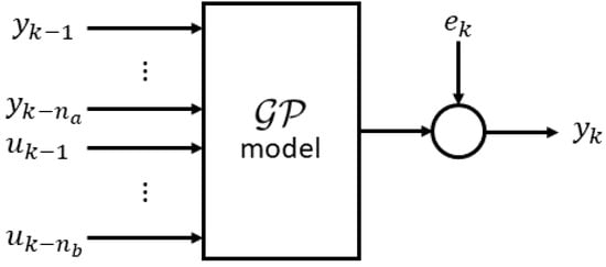
Figure 1.
GP-NARX scheme.
3.2. WANARX Model
The approximation capability associated with wavelet functions is well known, so a wavelet network is selected as a nonlinearity estimator for the NARX model. To compact the notation, the regressors vector is introduced:
where is the input delay. By rewriting Equation (11) according to the WANARX structure, one obtains:
where is the regressor mean, the p-by-1 vector of linear coefficients, an m-by-p projection matrix, l the scalar output offset, and
the nonlinear function constituted by dilated and translated wavelets and dilated and translated scaling functions (to improve the regularity of the estimator [23]). The nonlinear block and the linear block are combined together in a series-parallel structure to improve the estimation results.
Wavelets are functions located both in time and frequency. A finite energy signal can be decomposed into different frequency components by the superposition of functions obtained through scaling and translating an initial function known as the mother wavelet [23]. A radial function depending on the squared magnitude of vector x is chosen as the mother wavelet function for the relationship described by :
where
and is a m-by-q projection matrix, , the wavelet coefficients, the wavelet dilations parameters, the 1-by-q row vectors of wavelet translations, m the dimension of the regressors vector, the mean of and the total number of wavelets. For the relationship described by , a radial function is chosen as the scaling mother function:
where
in which are the scaling coefficients, the scaling dilations parameters, the 1-by-q row vectors of scaling translations, and the total number of scaling functions.
Structures in Equations (15) and (17) are very similar to the ones adopted by a neural network: a the wavelet network can be seen as a one-hidden-layer neural network with as the activation function of the hidden layer [24]. A schematic representation is reported in Figure 2.
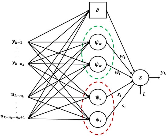
Figure 2.
WANARX scheme.
3.3. System Identification Process Overview
Experiments were carried out to create a training dataset consisting of system input–output data pairs. As for all black box identification approaches, the design of the experiment was carefully planned and the sampling time was carefully chosen. The aim of the data collection is to fully capture the system dynamics, since a model-based approach is proposed. The collected dataset was preprocessed (normalization, mean removal) to cancel the influence of different measuring scales and to reduce the weight of outliers.
The model structure selection was addressed by choosing the regressor vector form, basis functions, and their parameters. For the WANARX model, orders , and delay were selected. The covariance function and its hyperparameters were instead set for the GP-NARX model.
Fitting models to training data allows estimating the unknown parameters and obtaining the system model.The model quality must be tested through suitable validation criteria applied to a testing dataset, i.e., a set of independent input–output data collected during experiments and not used for training. It is common practice to split the collected dataset into two parts in order to have a training and a testing dataset and perform a model cross-validation.
In this paper, the root mean squared error (RMSE) between the predicted and measured output as well as the FIT percentage value were selected as quality indicators:
where is the predicted output, is the measured output, N is the number of samples and
The FIT is derived from the normalized root mean square error (NRMSE) using the relationship , where . The best model has the smaller RMSE and the higher FIT.
4. Experimental Validation
The objective is the identification of the PWM-angular velocity relationship that characterizes the motion of a small UGV equipped with tracks (Figure 3). The robotic platform is moved by two geared DC motors, one for the left and one for the right side, the behavior of which is assumed identical in this discussion. Each DC motor has an encoder integrated with the shaft. A pulse width modulation (PWM) technique is used for driving them: the signal is generated by a microcontroller, amplified by the H-bridge and used to power the motors and consequently move the tracks. The use of encoders allows the collection of the angular velocity, while the PWM duty cycle is obtained from the recording of the commands sent to the robot from a remote controller. The complexity of the system suggests the use of a black box approach instead of a classic lumped-parameter approach. In particular, a nonlinear model is selected to capture all nonlinearities and guarantee model fidelity. The model of the robot is completed by the introduction of a kinematic model (see [25]), which establishes the relationship between the angular speed of the tracks and the linear and angular velocities of the platform, thus giving the position and the orientation of the vehicle.
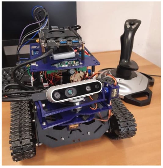
Figure 3.
Aerospace autonomous robots with onboard intelligent algorithms (STREAMS) Lab Robot (https://sites.google.com/view/streamrobotics-polito/home, accessed on 3 October 2022).
4.1. Experimental Setup
The data necessary for identification were collected, ranging over the whole space of the PWM duty cycle (from −20,000 s to 20,000 s). The goal was to define the relationship of the PWM and angular speed of the DC motor. The PWM values were selected as the model input u and the angular speed values as the model output y. A dataset of input–output vectors was created and observations were collected to train and test the dataset. The training dataset with input–output observation pairs was created from a 80 s long sample, in which the robot moved on a flat surface controlled by a radio controller. A sampling time of 0.2 s was adopted, which took into account the processing and communication capabilities of the robotic platform. A short mission of about 25 s was used to compare the model performance in the MATLAB environment.
4.2. WANARX Model
The WANARX model was trained using the MATLAB “System Identification Toolbox”. The available training dataset was normalized and arranged to create standard regressors with the structure reported below:
with , and . The choice of model orders was made based on a combination of prior knowledge of the system and trial and error. A five-unit wavelet network was implemented, with the main parameters reported in Table 1. A FIT value of 89.2388% with the training dataset was observed. In Figure 4, a comparison between the measured and predicted output was reported as validation upon a testing dataset of M = 128 data points.

Table 1.
WANARX parameters.
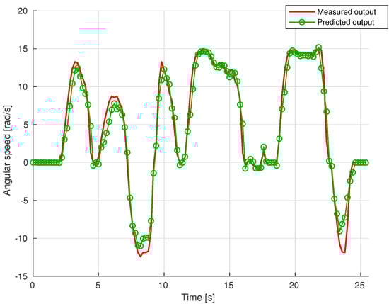
Figure 4.
Comparison between measured output (red line) and WANARX model predicted output (green line).
4.3. GP-NARX Model
The GP model was trained using the MATLAB “Statistics and Machine Learning Toolbox”, which finds the optimal hyperparameters maximizing the log-likelihood as well. A set of training inputs was created by rearranging the structure reported in Equation (12). Choosing = 3 and = 3, each input vector is as follows:
The output vector of training targets is equal to . A squared exponential kernel was selected (Equation (5) and its hyperparameters were established as reported in Table 2.
Table 2.
GP-NARX hyperparameters.
In Figure 5, the comparison between the measured and predicted output on the testing dataset was reported. Prediction intervals (95% confidence level) of the GP model predicted output are shown in Figure 6.
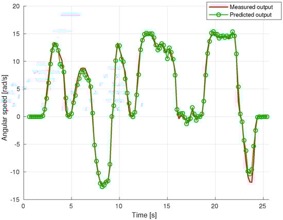
Figure 5.
Comparison between measured output (red line) and GP model predicted output (green line).
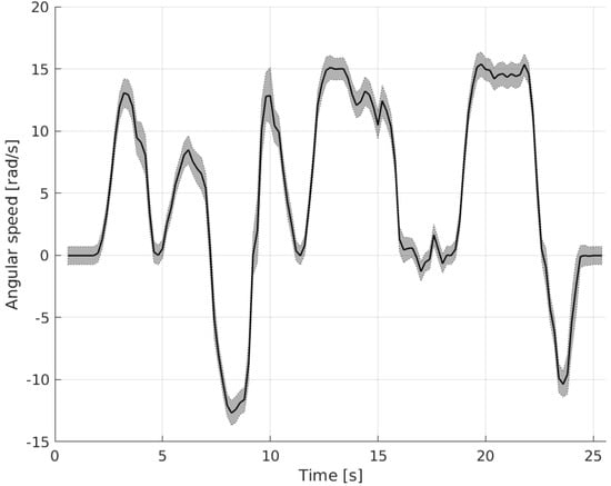
Figure 6.
Prediction intervals (95% confidence level) of GP model predicted output.
4.4. Discussion of Results
Figure 7 shows a comparison between the two proposed models. It can be noted that the GP model follows more accurately the measured shaft angular speed than the WANARX model, in particular during sharp changes. The overall performance was assessed using the quality indicators of Equations (19) and (20). The results are reported in Table 3. It can be observed that both models are characterized by a FIT value higher than 80%, with low RMSE values of 1.2955 rad/s for the WANARX model and 0.7169 rad/s for the GP-NARX. The GP-NARX model is more accurate in the prediction, with a high confidence in its estimation demonstrated by the narrow width of the uncertainty band around the average value.
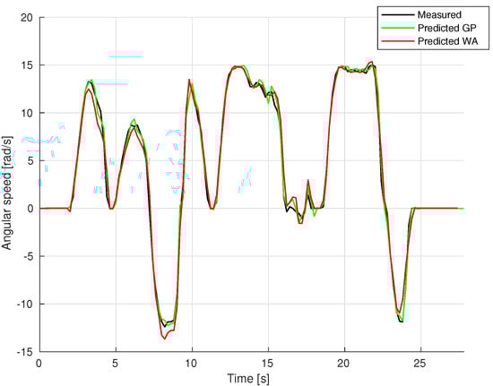
Figure 7.
Comparison between measured output (black line) and models predicted output (green line for GP-NARX, red for WANARX).
Table 3.
Performance comparison.
The performance of the WANARX model is also good but a lower performance can be observed compared with the GP method. Interesting considerations can be made if we look at the size of the training dataset: doubling the training samples and retraining the network while keeping the regressor structure unchanged, the FIT value refers to the same testing dataset rises to 88.1142% against a value of 92.457% for the GP-NARX. This shows that the WANARX model increases its predictive capability as the number of training points increases, but also that the GP is very effective even with small datasets. Both methods suffer from the “curse of dimensionality”, in particular the GP-NARX model doubles the execution time on the training dataset with respect to WANARX.
Nevertheless, it proves to be an accurate model for describing the relationship between PWM and angular velocity.
5. Discussion on Control System Design
If a nonlinear dynamic system is considered, the implementation limitations of control algorithms should be discussed. The control system design involves aspects related to robot dynamics, actuator behavior, noise characteristics, and an adequate modeling of these aspects is necessary for model-in-the-loop (MITL) or software-in-the-Loop (SITL) testing. The effectiveness of the control system depends strictly on the model on which the testing is carried out.
The selection of data driven identification techniques ensures that uncertainties in parameters; delays or constructive mechanical imperfections are included in the tuning of the control parameters during the simulation. The advantage lies in the possibility of employing both state-of-the-art techniques [26] and emerging ones (genetic algorithm (GA), particle swarm optimization (PSO) method, and artificial neural network (ANN) [27]) to obtain optimized gain factors on a faithful model of the system.
Here, we discuss the possibility of employing the model identified by the Gaussian process regression for control algorithm tuning.
GP models are widely employed together with model predictive control strategies. Advantages are linked to the computation of a prediction variance, which is an effective measure of the uncertainty of the learned model. They are less susceptible to overfitting, and they have, under certain circumstances, universal approximation capabilities for a large number of functions [28]. In [29], a model predictive control (MPC) based on a Gaussian process model was implemented for a pH neutralization process control example. An interesting aspect is the inclusion of variance information in the optimization process as a constraint to controller actions. In [30], a GP-based MPC framework was introduced in an overtaking scenario at highway curves. A GP model was developed to learn the unknown dynamics and to acquire information about the unexplored discrepancy between the nominal vehicle model and the real vehicle dynamics. The combination with a MPC strategy results in safe and stable control under changing friction road conditions. In [31], a learning-based control approach for underactuated balance robots was considered and a GP regression model was incorporated to enhance robustness to modeling errors.
In the case of an exam, a combination of a guidance and control algorithms, such as an artificial potential field (APF) and a proportional integrative derivative control (PID) have been implemented and tested using the previously introduced GP-NARX model. The performance of the system has been evaluated on the tracking capability of a reference signal generated in real time by the APF algorithm. Control requirements have been formulated in terms of rise time, settling time, overshoot, and steady state errors. The effectiveness of tuning has been demonstrated by the comparison between simulation data and experiments conducted with the robot.
6. Conclusions
In this paper, a Gaussian process regression model was proposed as nonlinear modeling technique for system identification for ground robots. The model was trained and validated using the robotic platform in our laboratory to assess its performance and its applicability to UGV dynamics modeling.
The GP framework was firstly introduced, then a practical implementation was reported to demonstrate the validity of the method alongside a classic NARX. In particular, a comparison was performed with a wavelet-based NARX model and some considerations about time effort and prediction accuracy on a test dataset were reported. The experimental results show that the GP model performance is better than the WANARX model. Moreover, GP-NARX models are able to provide the measure of uncertainty on the results. However, the training time is high due to the computational complexity of the matrix inversion. Finally, a brief discussion about different control strategies applied to data driven identification techniques was carried out. In particular, it was noted how the GP can effectively improve system performances in a great variety of engineering applications.
As part of future work, we propose the use of a recursive algorithm for the online estimation of the GP model and its hyperparameters. Indeed, the recursive GP method should be computationally efficient to be run on the robotic platform. Moreover, the system identification structures based on state-space representation will be considered.
Author Contributions
Conceptualization, E.I.T. and D.C.; methodology, E.I.T.; software, E.I.T. and D.C.; validation, E.I.T. and D.C.; resources, E.I.T.; data curation, E.I.T.; writing—original draft preparation, E.I.T. and D.C.; writing—review and editing, E.I.T., D.C., and E.C.; supervision, E.C.; project administration, E.C.; funding acquisition, E.C. All authors have read and agreed to the published version of manuscript.
Funding
This research received no external funding.
Institutional Review Board Statement
Not applicable.
Informed Consent Statement
Not applicable.
Data Availability Statement
Data available in a publicly accessible repository. The data presented in this study are openly available at https://github.com/DavideCarminati/GP-NARX_dataset.git, accessed on 3 October 2022.
Acknowledgments
We would like to thank Iris David Du Mutel for assistance during the experiments at our laboratory.
Conflicts of Interest
The authors declare no conflict of interest.
References
- Gregorcic, G.; Lightbody, G. Nonlinear system identification: From multiple-model networks to Gaussian processes. Eng. Appl. Artif. Intell. 2008, 21, 1035–1055. [Google Scholar] [CrossRef]
- Neal, R.M. Bayesian Learning for Neural Networks; Springer Science & Business Media: Berlin/Heidelberg, Germany, 2012; Volume 118. [Google Scholar]
- Williams, C.K.; Rasmussen, C.E. Gaussian Processes for Machine Learning; MIT Press: Cambridge, MA, USA, 2006; Volume 2. [Google Scholar]
- Kocijan, J.; Girard, A.; Banko, B.; Murray-Smith, R. Dynamic systems identification with Gaussian processes. Math. Comput. Model. Dyn. Syst. 2005, 11, 411–424. [Google Scholar] [CrossRef]
- Särkkä, S. The Use of Gaussian Processes in System Identification. arXiv 2019, arXiv:1907.06066. [Google Scholar]
- MacKay, D. InformationTheory, Inference, and Learning Algorithms. IEEE Trans. Inf. Theory 2003, 50, 2544–2545. [Google Scholar] [CrossRef]
- Ljung, L. System Identification: Theory for the User; Prentice Hall Information and System Sciences Series; Prentice Hall PTR: Hoboken, NJ, USA, 1999. [Google Scholar]
- Sjöberg, J.; Zhang, Q.; Ljung, L.; Benveniste, A.; Delyon, B.; Glorennec, P.Y.; Hjalmarsson, H.; Juditsky, A. Nonlinear black box modeling in system identification: A unified overview. Automatica 1995, 31, 1691–1724. [Google Scholar] [CrossRef]
- Pillonetto, G.; Dinuzzo, F.; Chen, T.; De Nicolao, G.; Ljung, L. Kernel methods in system identification, machine learning and function estimation: A survey. Automatica 2014, 50, 657–682. [Google Scholar] [CrossRef]
- Gotmare, A.; Bhattacharjee, S.S.; Patidar, R.; George, N.V. Swarm and evolutionary computing algorithms for system identification and filter design: A comprehensive review. Swarm Evol. Comput. 2017, 32, 68–84. [Google Scholar] [CrossRef]
- Chaudhary, N.I.; Raja, M.A.Z.; Khan, Z.A.; Mehmood, A.; Shah, S.M. Design of fractional hierarchical gradient descent algorithm for parameter estimation of nonlinear control autoregressive systems. Chaos Solitons Fractals 2022, 157, 111913. [Google Scholar] [CrossRef]
- Kocijan, J. Gaussian process models for systems identification. In Proceedings of the 9th International PhD Workshop on Systems and Control, Izola, Slovenia, 1–3 October 2008; pp. 8–15. [Google Scholar]
- Kocijan, J. Modelling and Control of Dynamic Systems Using Gaussian Process Models; Springer: Berlin/Heidelberg, Germany, 2016. [Google Scholar]
- Aftab, W.; Mihaylova, L. A Learning Gaussian Process Approach for Maneuvering Target Tracking and Smoothing. IEEE Trans. Aerosp. Electron. Syst. 2021, 57, 278–292. [Google Scholar] [CrossRef]
- Veibäck, C.; Olofsson, J.; Lauknes, T.R.; Hendeby, G. Learning Target Dynamics While Tracking Using Gaussian Processes. IEEE Trans. Aerosp. Electron. Syst. 2020, 56, 2591–2602. [Google Scholar] [CrossRef]
- Quinonero-Candela, J.; Rasmussen, C.E. A unifying view of sparse approximate Gaussian process regression. J. Mach. Learn. Res. 2005, 6, 1939–1959. [Google Scholar]
- Huber, M. Recursive Gaussian Process: On-line Regression and Learning. Pattern Recognit. Lett. 2014, 45, 85–91. [Google Scholar] [CrossRef]
- Schürch, M.; Azzimonti, D.; Benavoli, A.; Zaffalon, M. Recursive Estimation for Sparse Gaussian Process Regression. arXiv 2020, arXiv:1905.11711. [Google Scholar] [CrossRef]
- Girard, A. Approximate Methods for Propagation of Uncertainty with Gaussian Process Models; University of Glasgow: Glasgow, UK, 2004. [Google Scholar]
- Butler, A.; Haynes, R.D.; Humphries, T.D.; Ranjan, P. Efficient optimization of the likelihood function in Gaussian process modelling. Comput. Stat. Data Anal. 2014, 73, 40–52. [Google Scholar] [CrossRef]
- Titsias, M. Variational Learning of Inducing Variables in Sparse Gaussian Processes. In Proceedings of the Twelth International Conference on Artificial Intelligence and Statistics, Clearwater Beach, FL, USA, 16–18 April 2009; Volume 5, pp. 567–574. [Google Scholar]
- Snelson, E.; Ghahramani, Z. Sparse Gaussian Processes using Pseudo-inputs. In Proceedings of the 18th International Conference on Neural Information Processing System, Vancouver, BC, Canada, 5–8 December 2005; p. 8. [Google Scholar]
- Cajueiro, E.; Kalid, R.; Schnitman, L. Using NARX model with wavelet network to inferring the polished rod position. Int. J. Math. Comput. Simul. 2012, 6, 66–73. [Google Scholar]
- Zhang, Q. Using wavelet network in nonparametric estimation. IEEE Trans. Neural Netw. 1997, 8, 227–236. [Google Scholar] [CrossRef] [PubMed]
- Rached Dhaouadi, A.A.H. Dynamic Modelling of Differential-Drive Mobile Robots using Lagrange and Newton-Euler Methodologies: A Unified Framework. Adv. Robot. Autom. 2013, 2. [Google Scholar] [CrossRef]
- O’Dwyer, A. Handbook of PI and PID Controller Tuning Rules; Imperial College Press: London, UK, 2003. [Google Scholar]
- Prabhat Dev, M.; Jain, S.; Kumar, H.; Tripathi, B.N.; Khan, S.A. Various Tuning and Optimization Techniques Employed in PID Controller: A Review. In Proceedings of International Conference in Mechanical and Energy Technology: ICMET 2019, India; Yadav, S., Singh, D.B., Arora, P.K., Kumar, H., Eds.; Springer: Singapore, 2020; pp. 797–805. [Google Scholar] [CrossRef]
- Maiworm, M.; Limon, D.; Findeisen, R. Online learning-based model predictive control with Gaussian process models and stability guarantees. Int. J. Robust Nonlinear Control 2021, 31, 8785–8812. [Google Scholar] [CrossRef]
- Kocijan, J.; Murray-Smith, R.; Rasmussen, C.; Girard, A. Gaussian process model based predictive control. In Proceedings of the 2004 American Control Conference, Boston, MA, USA, 30 June–2 July 2004; Volume 3, pp. 2214–2219. [Google Scholar] [CrossRef]
- Liu, W.; Zhai, Y.; Chen, G.; Knoll, A. Gaussian Process based Model Predictive Control for Overtaking Scenarios at Highway Curves. In Proceedings of the 2022 IEEE Intelligent Vehicles Symposium (IV), IEEE, Aachen, Germany, 4–9 June 2022; pp. 1161–1167. [Google Scholar]
- Chen, K.; Yi, J.; Song, D. Gaussian Processes Model-Based Control of Underactuated Balance Robots. In Proceedings of the 2019 International Conference on Robotics and Automation (ICRA), Montreal, QC, Canada, 20–24 May 2019; pp. 4458–4464. [Google Scholar] [CrossRef]
Publisher’s Note: MDPI stays neutral with regard to jurisdictional claims in published maps and institutional affiliations. |
© 2022 by the authors. Licensee MDPI, Basel, Switzerland. This article is an open access article distributed under the terms and conditions of the Creative Commons Attribution (CC BY) license (https://creativecommons.org/licenses/by/4.0/).