Abstract
We show a successful numerical study of lid-driven square cavity flow with embedded circular obstacles based on the spectral/hp element methods. Various diameters of embedded two-dimensional circular obstacles inside the cavity and Reynolds numbers Re (from 100 to 5000) are considered. In order to verify the effectiveness and accuracy of the current methods, numerical results are investigated by comparing with those available in the literature obtained by the moving immersed boundary method (MIBM) and the lattice Boltzmann method (LBM). The present spectral/hp element methods have been not only successfully applied to study and visualize the primary and induced vortices but also capture new vortices on the lower right, upper left and upper right positions of the circular obstacle when Reynolds number Re = 100 and Re = 5000, which is not observed in the lattice Boltzmann method. The current data and figures are in good agreement with the published results. The results of the present study show that the spectral/hp element methods are effective and accurate in simulation of lid-driven cavity flow with embedded circular obstacles, and the present methods have the following advantages: less preprocesses required and high-resolution characteristics.
1. Introduction
The lid-driven square cavity flow is an internal recycling flow generated by one or more wall movements. Although the model of lid-driven square cavity is relatively simple, almost all possible flow phenomena (for example, eddies, secondary flows, Taylor–Görtler-like vortex, fluid bifurcation, instabilities, transients and turbulence, etc.) in the incompressible fluid can be observed in the lid-driven square cavity flow. Therefore, the lid-driven square cavity flow can be utilized to analyze many important theoretical and engineering problems. Numerical studies of the lid-driven square cavity flow have many applications in practical engineering, such as in the meteorology, navigation, mechanology and mining, etc. The lid-driven square cavity flow has been one of the classical problems in research of the incompressible fluid flow.
In the past several decades, there were a lot of studies about the lid-driven square cavity flow using different numerical approaches, for example, the implicit multigrid method (BIMM) [1,2], the p-type finite element method [3], Chebyshev collocation method [4], stream function–velocity formulation [5,6], the moving immersed boundary method (MIBM) [7,8,9] and the lattice Boltzmann method [10,11,12,13], etc. Among the methods mentioned above, the most commonly used method is the lattice Boltzmann method. Although many results about the lid-driven square cavity flow have been obtained using different numerical methods, only a few studies are focused on the more complex aspect of the lid-driven square cavity flow with an embedded obstacle. Recently, Cai et al. [8] investigated the fluid flow problem of the lid-driven square cavity flow with an embedded cylinder in the domain center using the moving immersed boundary method, and compared results with the body-conforming mesh method. Huang et al. [13] applied the lattice Boltzmann method to study the lid-driven square cavity flow inside cavities with internal circular obstacles for various Reynolds numbers Re (Re is between 100 to 5000).
In the field of industrial applications, Gamaoun et al. [14] studied T91 steel specimens in liquid lead. They described the various specimens and treatment conditions either giving rise to the cavitation effect or not. Sarris et al. [15,16] investigated numerically laminar free convection flow in a square enclosure driven by magnetic forces and MHD natural convection in a laterally and volumetrically heated square cavity. In this paper, we only consider the classical lid-driven square cavity flow with embedded circular obstacles instead of considering heat exchanges.
The spectral/hp element methods incorporate both the spectral method and the hp-version finite element method, and combine the flexibility of the classical finite element solution domain with the faster convergence and higher accuracy of the spectral method. Theoretically, the spectral/hp element methods can provide an arbitrary order of accuracy in spatial discretization requiring relatively lower computational cost. Hence, in recent years, the spectral/hp element methods have attracted more and more attention and have been widely used in academia and engineering, especially in computational fluid dynamics (CFD), see [17,18,19,20,21,22,23]. Although the spectral/hp element methods have been extended to various engineering fields, as far as we know, few research of lid-driven square cavity flow with embedded obstacles using the high-order method can be found in the existing literature.
This study aims to apply the spectral/hp element methods of high accuracy and efficiency to simulate the flow inside a square cavity with embedded two-dimensional circular obstacles. The computational tool used in the simulation is an open source spectral/hp element framework: Nektar++5.0.1 [24]. In order to show the less preprocess requirements and high-resolution characteristics of the present methods, we compare current results with Cai et al. [8] and Huang et al. [13] and adopt the same parameters and the boundary conditions (various diameters and different Reynolds numbers Re (Re is between 100 to 5000)) in numerical models. The effectiveness and accuracy of current methods are demonstrated by numerical models.
2. Spectral/hp Element Methods
2.1. Governing Equation
For the dimensionless incompressible N-S equations for a viscous Newtonian fluid, the continuity equation and momentum equation can be written as follows:
where , , , and are the fluid velocity vector, fluid density, the pressure, the kinematic viscosity of fluid and the body force, respectively. The dimensionless Reynolds number , where is the lid motion velocity and is the length of cavity. For simplicity, we suppose the fluid density .
2.2. Spectral/hp Element Methods
A detailed content of the spectral/hp element methods can refer to Karniadakis et al. and Szabó et al. [25,26].
Generally, for the partial differential equations (PDEs), , which is defined on a domain , the domain is divided into n-dimensional finite element meshes , n = 1, 2, 3, , . We seek the weak solution of the PDEs , (Sobolev space). We find such that , , where is a symmetric bilinear form, is a linear form, and is a Sobolev space, which is defined as follows:
In a finite dimensional subspace , we seek such that , ; in order to keep continuity across elements, is required. Suppose can be written as a linear combination of trial functions , i.e.,, where is defined on . Then, the problem converts to determining the coefficients . Next, the residual are restricted so that its inner product is zero with respect to the test functions . As it is well known to all, for the Galerkin projections, we let .
For the construction of the global basis functions , the contributions from every element in the solution domain should be considered. We mapped every into a standard element (n = 1, 2, 3) by an isoparametric mapping. Similarly, the mappings of high-order elements can refer to Szabó et al. [26].
We denote the space as the polynomials space of order p defined on the standard element . In one-dimensional case, the local polynomial basis functions on each standard element can be constructed by the following hierarchical basis functions [25]:
where is defined by the following Legendre polynomial ,
In two- and three-dimensional cases, the tensorial basis functions are used, which are derived as the tensor-product of the one-dimensional basis functions on one-dimensional, two-dimensional or three-dimensional elements. If we define the local polynomial basis functions by the Lagrange interpolation polynomials, then it will lead to the spectral element method.
2.3. High-Order Splitting Scheme
Consider the incompressible N-S equations for viscous Newtonian fluids governed by the following:
where denotes the velocity vector, is the pressure, is the kinematic viscosity of fluid, and is the body force.
From [27,28], the high-order splitting scheme can be divided into two steps:
- Firstly, we derived the weak pressure approximation as follows:
This equation can be written as an equivalent strong form of the pressure Poisson equation:
with consistent Neumann boundary conditions
- 2.
- Secondly, we discretize the Equation (4) at time step and solve the velocity by using the pressure at step from step 1. Now the approximation of the time derivative is:
Then, the Helmholtz problem is derived as follows:
The Helmholtz problem can be solved. A detailed discussion can be found in [25,27,28].
In this paper, the governing equations are discretized by using the spectral/hp element methods. The spatial discretization is performed by using orthogonal polynomials, for example, Legendre or Chebyshev polynomials. The time discretization is performed by using the high-order splitting scheme. A detailed analysis of the high-order splitting scheme can refer to [27,28].
3. Numerical Examples
3.1. Lid-Driven Square Cavity Flow with an Embedded Circular Obstacle
We consider the classical lid-driven square cavity flow, except an embedded circular obstacle is placed in the domain center. Figure 1 shows the parameters and configuration of the model. In order to demonstrate the validation and performance of current approaches, we implement the same parameters and the boundary conditions as Cai et al. [8] and Huang et al. [13], namely the top lid moves toward the right with a uniform horizontal velocity ; the boundary conditions are all non-slip wall conditions, on .
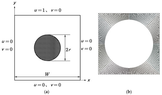
Figure 1.
The lid-driven square cavity flow with an embedded circular obstacle. (a) Model (b) Meshes.
3.2. Results and Discussion
Figure 2 displays the comparison of vorticity contours and streamlines with Cai et al. [8] at radius , Reynolds number . As we can see from Figure 2, three vortices appeared in the lid-driven square cavity. One is at the upper right corner of the circular obstacle and the other two vortices locate at the bottom lower left and right corners. These results are similar to those of [8]. The only difference is that the immersed boundary method identifies the internal circular obstacle as a fluid. The center coordinates of the three vortices are also listed in Table 1. Compared with the data in Cai et al. [8], the relative errors of this paper are less than 1.8%. It is worth noting that the total mesh number of 200 × 200 is used in [8] applying the immersed boundary method, but the total number of meshes used in the spectral/hp element methods is 4864, which shows that the present method is accurate and effective for the numerical investigation of the lid-driven square cavity flow with an embedded circular obstacle, and with lesser preprocess costs.
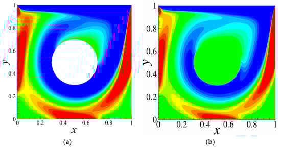
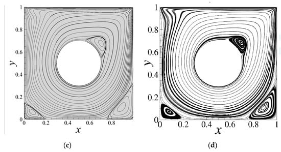
Figure 2.
Vorticity contours and streamlines at , . (a) Vorticity (Present) (b) Vorticity (Cai et al. [8]) (c) Streamlines (Present) (d) Streamlines (Cai et al. [8]).

Table 1.
Comparison of vortice center coordinates with the moving immersed boundary method (at , ).
Figure 3 shows the comparison of the horizontal and vertical velocity of the lid-driven square cavity flow with an embedded circular obstacle at different Reynolds number with Huang et al. [13]. The results are similar to those of [13].
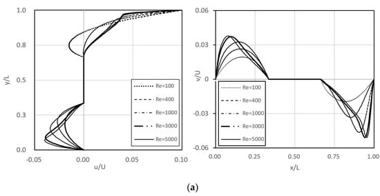
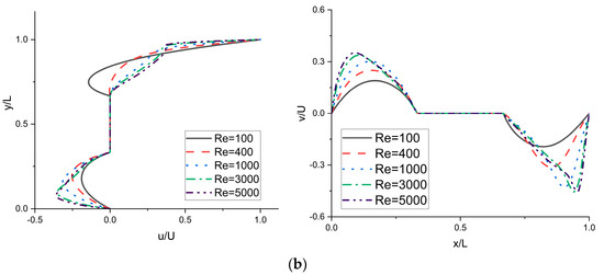
Figure 3.
Comparison of the profiles of u-velocity and v-velocity in the lid-driven square cavity flow with an embedded circular obstacle at various Reynolds numbers. (a) The profiles of u-velocity and v-velocity alone and (Huang et al. [13]). (b) The profiles of u-velocity and v-velocity alone and (Present).
In order to evaluate the characteristics of flow around obstacles in a lid-driven square cavity with an embedded circular obstacle, the variations of the flow are numerically simulated at radius and Reynolds number , respectively. The numbers of meshes used in the simulation are 7168, 4096, 4864, 6376 and 1536 corresponding to radius , respectively. Since the computational domain varies with the cylinder radius, the number of meshes also varies with the different division of meshes. The order of interpolated polynomial on individual grid is different when using the adaptive hierarchical techniques; because the upper and lower limits of tolerance are the same for all cases, the computational accuracy is guaranteed.
Figure 4 displays the variation of the flow in the lid-driven square cavity for different Reynolds numbers at the radius . As we can see from Figure 4, with the increase in Re, the vortex at the bottom of the square cavity gradually grows in size.
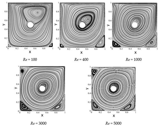
Figure 4.
Streamlines of the lid-driven square cavity flow with an embedded circular obstacle at various Reynolds numbers at
.
The center of the vortex at the upper right side of the cavity gradually approaches to the boundary of the internal obstacle and decreases. When Re is greater than 3000, a new vortex appears on the upper left position of the cavity, and the corner vortex becomes larger with the increase in Re.
Figure 5 displays the variation of the flow in the lid-driven square cavity at different Reynolds numbers at the radius . As it can be seen in Figure 5, with the increase in Re, the corner vortex at the bottom gradually grows in size. The center of the vortex at the upper right position of the cavity gradually approaches the boundary of the embedded obstacle and decreases. When Re is greater than 3000, an induced vortex appears on the upper left position of the cavity, and the induced vortex becomes larger with the increase in Re. However, in the results obtained by Huang et al. [13] using the lattice Boltzmann method, the corner vortex in the lower right corner of the square cavity is not observed at Re = 100. Owing to the higher-order properties of the method used here, the present spectral/hp element methods successfully capture the third vortex on the lower right corner of the cavity, and the vortex on the lower right corner is clearly visible.
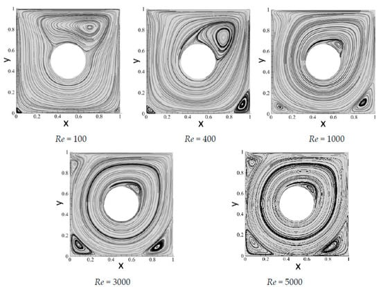
Figure 5.
Streamlines of the lid-driven square cavity flow with an embedded circular obstacle at different Reynolds numbers Re at .
Figure 6 shows the streamlines in the lid-driven square cavity at different Reynolds numbers Re at the radius . At this radius, the characteristics of the flow in the square cavity at various Reynolds numbers are essentially the same as at the radius . With the increase in Re, the corner vortex at the two sides of bottom gradually expand, but the vortex in the upper right corner of the square cavity gradually becomes smaller. Compared to the streamlines at , the primary vortex at the upper position of the embedded obstacle in the cavity tends to elongate to some extent in the case of Re = 100.
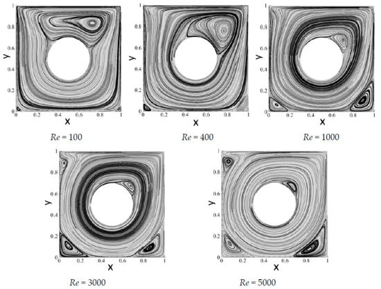
Figure 6.
Streamlines of the lid-driven square cavity flow with an embedded circular obstacle at various Reynolds numbers at .
We continue to increase the radius ; when , the primary vortex at the upper position of the internal obstacle in the cavity gradually splits into two vortices. However, with the increase in the Reynolds number, these two vortices merge again into a vortex gradually contracting towards the upper right position of the embedded obstacle. The induced vortices on the upper left side of the cavity also expand with the increase in Re, as displayed in Figure 7. In the case of , Re = 100, the number of meshes is 4096 and the tolerance is set to , the time required to arrive to a steady state of CPU (a single core) is 1652 s.
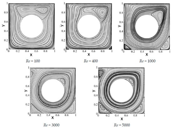
Figure 7.
Streamlines of the lid-driven square cavity flow with an embedded circular obstacle at different Reynolds numbers Re at .
When the radius of the embedded circular obstacle becomes larger due to the strengthening of the wall effect, at , the upper primary vortex in the cavity transforms almost into two corner vortices, as shown in Figure 8. With the increase in Re, the two vortices on the upper region of the square cavity do not show the merger of the vortices as at instead, a small-scale vortex on the upper left side and a large-scale vortex on the upper right of the obstacle are formed by gradual contraction.
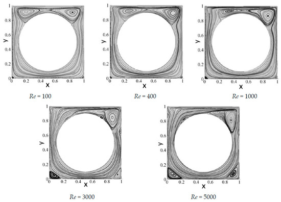
Figure 8.
Streamlines of the lid-driven square cavity flow with an internal circular obstacle at different Reynolds numbers at .
Two newly induced vortices are observed on the upper left and right sides of the circular obstacle, respectively. This result is different from the result in Huang et al. [13]; the lattice Boltzmann method cannot capture these new vortices in [13]. This also shows the high-resolution characteristics of the spectral/hp element methods.
Figure 9 displays the vorticity contours for the different radius at . As we can see from the figure, for all the cases of radius , the larger absolute values of vorticity () appear in the thin shear layer region near the walls of the cavity and walls of the obstacle, the absolute value of the maximum vorticity appears in the top corner region of the upper left and right corners of the cavity, and the vorticity on the upper side in the top corner region is negative, whilw the vorticity on the underside at the top corner region is positive. For the smaller Reynolds numbers, the radius has no substantial effect on the vorticity distribution. The distribution of vorticity inside the square cavity is similar at different radii; however, the radius of the embedded circular obstacle has an important effect on the vorticity inside the cavity. The variation of the Re has a great influence on the square cavity flow with an embedded circular obstacle. At a higher Reynolds number (Re = 5000), the absolute value of vorticity () is larger in the near wall area and the area surrounding the circular obstacle, as shown in Figure 10.
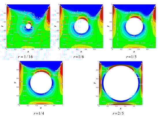
Figure 9.
Vorticity contours for various at .
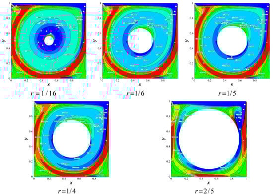
Figure 10.
Vorticity contours for various at .
4. Conclusions
In the paper, the lid-driven square cavity flow with embedded circular obstacles was numerically simulated by using spectral/hp element methods. The variation of the flow at various diameters of internal two-dimensional circular obstacles inside the cavity and Reynolds numbers were investigated. Numerical results were analyzed and compared with the available data in the literature to validate the performance and accuracy of the current methods. The conclusions of this paper can be summarized as follows:
- The stream function and the locations of the primary and secondary vortices obtained by the present methods are compared with published data. These results are in very good agreement with existing results. The validity of the numerical solution is verified.
- The simulation based on the spectral/hp element methods only needs less preprocessing, has higher accuracy, which can be used not only to analyze the lid-driven square cavity flow but also other 2D and 3D incompressible viscous flows.
- The main advantages of the spectral/hp element methods are high-resolution characteristics and less preprocessing required. The spectral/hp element methods capture new vortices in numerical analysis of the lid-driven square cavity flow with embedded two-dimensional circular obstacles at , and , (see Figure 5 and Figure 8). However, these new vortices cannot be observed in the lattice Boltzmann method.
- Although the spectral/hp element methods have the advantages of less preprocessing, high-resolution characteristics and faster convergence rate, due to the use of high-order interpolation, despite the hierarchic type shape functions being employed, higher computation cost is still inevitable. Hence, it is an important to balance between accuracy and computation cost.
Author Contributions
Conceptualization, J.Z. and B.X.; methodology, J.Z.; software, W.Y. and B.X.; validation, J.Z., B.X. and W.Y.; formal analysis, J.Z. and W.Y.; investigation, B.X.; resources, B.X.; data curation, W.Y.; writing—original draft preparation, J.Z.; writing—review and editing, J.Z. and B.X.; visualization, B.X. and W.Y. supervision, J.Z.; project administration, J.Z.; All authors have read and agreed to the published version of the manuscript.
Funding
This research was funded by the National Natural Science Foundation of China (Grant No. 51769011).
Institutional Review Board Statement
Not applicable.
Informed Consent Statement
Not applicable.
Data Availability Statement
Data is contained within the present article. Other data presented in this research are available in [8,13].
Conflicts of Interest
The authors declare no conflict of interest.
Nomenclature
| symmetric bilinear form | |
| coefficients | |
| body force | |
| linear form | |
| Sobolev space | |
| length of cavity | |
| fluid pressure | |
| test function | |
| r | radius |
| Re | Reynolds numbers |
| finite dimensional subspace | |
| t | time |
| fluid velocity vector | |
| lid motion velocity | |
| u, v | velocity components in x and y directions |
| x, y | spatial coordinates |
| Greek symbols | |
| kinematic viscosity of fluid | |
| fluid density | |
| computational domain | |
| trial functions | |
| test functions | |
| constant | |
| Subscripts and superscripts | |
| n | the number of iteration |
| the ith element |
References
- Ghia, U.; Ghia, K.N.; Shin, C.T. High-Re solutions for incompressible flow using the Navier-Stokes equations and a multigrid method. J. Comput. Phys. 1982, 48, 387–411. [Google Scholar] [CrossRef]
- Wright, N.G.; Gaskell, P.H. An efficient Multigrid Approach to Solving Highly Recirculating Flows. Comput. Phys. 1995, 24, 63–79. [Google Scholar] [CrossRef]
- Barragy, E.; Carey, G.F. Stream Function-Vorticity Driven Cavity Solutions Using p Finite Elements. Comput. Phys. 1997, 26, 453–468. [Google Scholar] [CrossRef]
- Botella, O.; Peyret, R. Benchmark Spectral Results on the Lid-Driven Cavity Flow. Comput. Phys. 1998, 27, 421–433. [Google Scholar] [CrossRef]
- Gupta, M.M.; Kalita, J.C. A new paradigm for solving Navier-stokes equations, streamfunction-velocity formulation. J. Comput. Phys. 2005, 207, 25–68. [Google Scholar] [CrossRef]
- Erturk, E.; Corke, T.; Gokcol, C. Numerical Solutions of 2-D Steady Incompressible Driven Cavity Flow in a driven skewed cavity High Reynolds Numbers. Int. J. Numer. Methods Fluids 2005, 48, 747–774. [Google Scholar] [CrossRef]
- Cai, S.G.; Ouahsine, A.; Favier, J.; Hoarau, Y. Improved implicit immersed boundary method via operator splitting. In Computational Methods for Solids and Fluids; Ibrahimbegovic, A., Ed.; Springer: Berlin/Heidelberg, Germany, 2016; pp. 49–66. [Google Scholar] [CrossRef]
- Cai, S.G.; Ouahsine, A.; Favier, J.; Hoarau, Y. Moving immersed boundary method. Int. J. Numer. Methods Fluids 2017, 85, 288–323. [Google Scholar] [CrossRef]
- Zhu, J.; Holmedal, L.E.; Wang, H.; Myrhaug, D. Flow patterns in a steady lid-driven rectangular cavity with an embedded circular cylinder. Fluid Dyn. Res. 2020, 52, 6. [Google Scholar] [CrossRef]
- Hou, S.; Zhou, Q.; Chen, S.; Doolen, G.; Cogley, A.C. Simulation of cavity flow by the lattice Boltzmann method. J. Comput. Phys. 1995, 118, 329–347.5. [Google Scholar] [CrossRef]
- Guo, Z.L.; Shin, B.C.; Wang, N. Lattice BGK model for incompressible Navier-Stokes equation. J. Comput.Phys. 2000, 165, 288–306. [Google Scholar] [CrossRef]
- Aslan, E.; Taymaz, I.; Benim, A.C. Investigation of the Lattice Boltzmann SRT and MRT Stability for Lid Driven Cavity Flow. J. Mater. Mech. Manuf. 2014, 2, 317–324. [Google Scholar] [CrossRef]
- Huang, T.T.; Lim, H.C. Simulation of Lid-Driven Cavity Flow with Internal Circular Obstacles. Appl. Sci. 2020, 10, 4583. [Google Scholar] [CrossRef]
- Gamaoun, F.; Dupeux, M.; Ghetta, V.; Gorse, D. Cavity formation and accelerated plastic strain in T91 steel in contact with liquid lead. Scr. Mater. 2004, 50, 619–623. [Google Scholar] [CrossRef]
- Sarris, I.E.; Grigoriadis, D.G.E.; Vlachos, N.S. Laminar free convection in a square enclosure driven by the Lorentz force. Numer. Heat Transf. Part A Appl. 2010, 58, 923–942. [Google Scholar] [CrossRef]
- Sarris, I.E.; Kakarantzas, S.C.; Grecos, A.P.; Vlachos, N.S. MHD natural convection in a laterally and volumetrically heated square cavity. Int. J. Heat Mass Transf. 2005, 48, 3443–3453. [Google Scholar] [CrossRef]
- Sherwin, S.J.; Ainsworth, M. Unsteady Navier–Stokes solvers using hybrid spectral/hp element methods. Appl. Numer. Math. 2000, 33, 357–363. [Google Scholar] [CrossRef]
- Pontaza, J.P.; Reddy, J.N. Space–time coupled spectral/hp least-squares finite element formulation for the incompressible Navier–Stokes equations. J. Comput. Phys. 2004, 197, 418–459. [Google Scholar] [CrossRef]
- Kirby, R.M.; Sherwin, S.J. Stabilisation of spectral/hp element methods through spectral vanishing viscosity: Application to fluid mechanics modelling. Comput. Methods Appl. Mech. Eng. 2006, 195, 3128–3144. [Google Scholar] [CrossRef]
- Mengaldo, G.; Grazia, D.D.; Moxey, D.; Vincent, P.E.; Sherwin, S.J. Dealiasing techniques for high-order spectral element methods on regular and irregular grids. J. Comput. Phys. 2015, 299, 56–81. [Google Scholar] [CrossRef]
- Gonzalez, L.; Ferrer, E.; Diaz-Ojeda, H. Onset of three-dimensional flow instabilities in lid-driven circular cavities. Phys. Fluids 2017, 29, 64102. [Google Scholar] [CrossRef]
- Moura, R.C.; Peiró, J.; Sherwin, S.J. Implicit LES approaches via discontinuous Galerkin methods at very large Reynolds. In Direct and Large-Eddy Simulation XI; Salvetti, M., Armenio, V., Frohlich, J., Geurts, B., Kuerten, H., Eds.; Springer: Berlin/Heidelberg, Germany, 2019; pp. 53–59. [Google Scholar] [CrossRef]
- Mengaldo, G.; Moxey, D.; Turner, M.; Moura, R.C.; Jassim, A.; Taylor, M.; Peiró, J.; Sherwin, S.J. Industry-Relevant Implicit Large-Eddy Simulation of a High-Performance Road Car via Spectral/hp Element Methods. SIAM Rev. 2021, 64, 723–755. [Google Scholar] [CrossRef]
- Available online: http://www.nektar.info (accessed on 8 October 2022).
- Karniadakis, G.E.; Sherwin, S.J. Spectral/hp Element Methods for Computational Fluid Dynamics, 2nd ed.; Oxford University Press: Oxford, UK, 2005; ISBN 9780199671366;0199671362. [Google Scholar]
- Szabó, B.; Babuška, I. Introduction to Finite Element Analysis: Formulation, Verification and Validation; John Wiley & Sons: Hoboken, NJ, USA, 2011; ISBN 978-1-119-99348-3. [Google Scholar]
- Karniadakis, G.E.; Israeli, M.; Orszag, S.A. High-order splitting methods for the incompressible Navier–Stokes equations. J. Comput. Phys. 1991, 97, 414–443. [Google Scholar] [CrossRef]
- Guermond, J.L.; Shen, J. Velocity-correction projection methods for incompressible flows. SIAM J. Numer. Anal. 2003, 41, 112–134. [Google Scholar] [CrossRef]
Publisher’s Note: MDPI stays neutral with regard to jurisdictional claims in published maps and institutional affiliations. |
© 2022 by the authors. Licensee MDPI, Basel, Switzerland. This article is an open access article distributed under the terms and conditions of the Creative Commons Attribution (CC BY) license (https://creativecommons.org/licenses/by/4.0/).