Abstract
Images taken on rainy days often lose a significant amount of detailed information owing to the coverage of rain streaks, which interfere with the recognition and detection of the intelligent vision systems. It is, therefore, extremely important to recover clean rain-free images from the rain images. In this paper, we propose a rain removal method based on directional gradient priors, which aims to retain the structural information of the original rain image to the greatest extent possible while removing the rain streaks. First, to solve the problem of residual rain streaks, on the basis of the sparse convolutional coding model, two directional gradient regularization terms are proposed to constrain the direction information of the rain stripe. Then, for the rain layer coding in the directional gradient prior terms, a multi-scale dictionary is designed for convolutional sparse coding to detect rain stripes of different widths. Finally, to obtain a more accurate solution, the alternating direction method of multipliers (ADMM) is used to update the multi-scale dictionary and coding coefficients alternately to obtain a rainless image with rich details. Finally, experiments verify that the proposed algorithm achieves good results both subjectively and objectively.
1. Introduction
Images and videos captured on rainy days are easily blurred by the scattering of raindrops, which significantly limits the performance of outdoor visual processing systems, such as image segmentation, target recognition, and target tracking. Most previous studies have focused on video image rain removal [1,2,3,4,5,6,7,8] by using prior information among the related frames [5,7]. However, due to the need to obtain more information for detecting and removing rain streaks from adjacent frames, video image rain removal methods are unsuitable for single image rain removal. In recent years, single image rain removal has attracted more attention from academics, and its ideas can be roughly divided into three categories: sparse-coding- [9,10,11,12,13,14,15], filter- [16,17,18], and deep learning-based methods [19,20,21,22].
The main idea of the sparse-coding-based rain removal method is firstly to decompose the rain image into low-frequency and high-frequency parts by reasonably describing the rain removal problem as an image decomposition problem; then, the accurate rain component is obtained from the high-frequency part by analyzing the internal structure of the image in the sparse domain; finally, the rain-free image is obtained by stripping the rain component from the rain image. As early as 2012, Kang et al. [9] proposed a single image rain removal method based on sparse coding, which successfully removed the rain component from the rain image by performing dictionary learning and sparse coding. Similarly, Chen et al. [10] decomposed the rain image into low-frequency and high-frequency parts by using the guided image filter, and then employed a hybrid feature set for dictionary learning and sparse coding to extract non-rain components from the high-frequency part. Luo et al. [11] adopted a nonlinear rain model to remove rain streaks by constraining the correlation between the sparse coefficients of the rain components and rainless images. On the basis of image decomposition, Li et al. [12] further proposed an effective method using patch prior knowledge based on a Gaussian mixture model (GMM) to separate a rain layer and a rainless layer from a rain image. To better extract the information of rain streaks, Gu et al. [14] proposed a sparse representation model based on analysis sparse representation (ASR) and composite sparse representation (CSR), which can more effectively utilize the global information of the image through a convolution operation. In 2017, Wang et al. [15] proposed a hierarchical rain detection method that utilizes a rain detection matrix and a guided filter to separate the rain layer information from a rain image. When the prior information of the rain layer can be fully utilized, the rain removal methods based on sparse coding can detect the rain layer information better and remove the rain layers from rain images. However, due to the lack of prior information of the rain layer, most of the existing methods have problems, such as the loss of the original details of the image and the residue of rain streaks in the rain removal results, leading to the unnatural artifacts and fuzzy image edges in the restored image.
The filter-based rain removal method removes the rain layer by filtering rain images according to the structural features of the rain signals. Xu et al. [16] proposed a rain removal algorithm based on guided filtering (GF), which considers the rain patterns to have an almost equal influence on each pixel in the RGB color channels and filters the three channels to obtain the final rainless image. Zheng et al. [17] proposed a new method for removing the rain and snow by applying the low-frequency component of a single image, in which the low-frequency component containing a no-rain or no-snow component is used as a guide image to filter the high-frequency component. The filtered high-frequency component is combined with the low-frequency component to obtain the restored image. However, owing to the simple weighting of the high- and low-frequency components, the results of the high-frequency component are inaccurate, resulting in poor visual effect of the restored image. Ding et al. [18] proposed a rain removal method based on a smoothing filter l0. In this method, the rain image and its corresponding low frequency are filtered by the smooth filter l0, and the result is compared with the original rain image by considering the minimum gray values as pixels of a rainless image. A rainless image recovered using this method is relatively clear, although some rain streaks are still retained. Because of the inherent overlap between the rain streaks and the background texture, most filter-based methods not only remove the rain streaks but also remove the texture details of the rainless area, resulting in an excessive smoothing effect in the restored background.
Due to the powerful learning ability of deep convolution networks, deep learning has been used in many fields of computer vision, such as classification [19,20,21], pattern recognition [22,23], and target detection [24,25]. Similarly, deep learning has made great progress in the task of rain removal [26,27,28,29]. Fu et al. [26] proposed a deep detail network (DetailsNet) based on a deep convolutional neural network (CNN) to directly reduce the mapping range from a rainy image to a rainless image. Zhang et al. [27] proposed a new multi-stream dense connection CNN, which can automatically determine the rain density information and effectively remove the corresponding rain streaks under guidance of the estimated rain density label. Fu et al. [28] also proposed a lightweight rain removal network (LPNet), which can obtain rainless images more quickly and significantly reduce the storage space required by the model. Hu et al. [29] designed a lightweight deep convolutional neural network with the depth-guided non-local (DGNL) module to realize rain streaks and fog removal from the input rainy images. The rain removal methods based on deep learning have made significant progress and achieved good results. However, these methods require a large amount of sample data to drive the network training, and the sample data can be obtained only by using the degradation model to simulate the rain formation process. However, the imaging process of rain images of natural scenery is extremely complex. Most of the methods commonly used in the existing rain models cannot fully describe the internal mechanism of rain image degradation. Therefore, obtaining more real sample data is one of the greatest difficulties of a deep learning method. Similarly, the training of the network model and the adjustment of the model parameters also affect the network performance.
To remove rain streaks from rain images and retain as much structural information of the original rain images as possible, we propose a single image rain removal method based on directional gradient priors. According to the directionality of the rain streaks and the sparsity of the rain layer gradient maps, two gradient sparse regularization terms are constructed to constrain the solution of the rain layer. To extract the structure of the rain streaks more accurately, a sparse coding method based on multi-scale dictionaries is proposed to encode the rain layer and realize a refinement of the rain layer solution. Because the parameters of the model are constrained by multiple constraint terms, the ADMM algorithm is used to solve the model alternately to obtain a rainless image with rich details.
Our main contributions are as follows:
- A rain removal method based on directional gradient priors is proposed, which can better optimize the rain layer and obtain a rainless layer (i.e., background layer) with richer texture.
- By analyzing the structure of rain streaks, the horizontal gradient and vertical gradient prior constraints of rain layer are constructed to detect more accurate rain layer information.
- Considering that the rain streaks have a variety of sizes, multi-scale dictionaries are designed to encode and refine the rain layer.
- To solve the rain removal model, the ADMM method is derived to alternately solve the background layer and rain layer of the rainy image.
The remainder of this article is structured as follows. In Section 2, we summarize the related work on rain removal theory and the sparse representation of a single image. In Section 3, the proposed model is introduced in detail. In Section 4, experiments comparing the proposed model with several main-stream methods are carried out on both synthetic and real images. Finally, we provide some concluding remarks in Section 5.
2. Related Work
The traditional single image rain removal method regards a rain image as a superposition of background layer and rain layer, and thus the rain model can be described as follows:
where represents a rain image, is the background layer, and is the rain layer. According to the requirement of the layer separation, the existing methods were proposed to standardize the stratified results with different priors. As a powerful image prior model, the sparsity prior has been widely used in different layer separation applications [11,30].
Y = B + R
A sparse representation of the images is derived from the hypothesis of efficient neuron coding, and the human visual system adopts a low-energy metabolic information processing strategy for an external input signal, namely sparse coding [30,31]. From the perspective of image processing, sparse coding simulates the sparse activity characteristics of physiological neurons and uses a group of atomic bases to sparsely represent the input image. In short, sparse coding is a linear combination of a large number of samples represented by a set of basis vectors [6,31]. The coefficients corresponding to the basis vectors are sparse, that is, they contain only a few non-zero elements or a few elements far greater than zero. The general form of the sparse coding can be defined as follows:
where y is the encoded data, x is the sparse vector to be estimated, λ represents the regularization parameter, and is a sparse measure.
The key to a sparse representation is to find the basis of a sparse representation of the signal [32,33,34]. The sparse representation of a signal can be obtained by the following two types: traditional sparse coding and convolutional sparse coding. Traditional sparse coding requires searching for a suitable dictionary from multiple redundant dictionaries trained to represent the same feature, whereas convolutional sparse coding uses the dictionary shared by all samples as the convolution kernel, which can capture the noise signal. The advantages of convolutional sparse coding can be summarized as the following four points [35,36,37]. First, convolution sparse coding can use a filter to form a dictionary, which is faster in execution, and the learning algorithm is not limited by the size of the image block. Second, convolution coding can capture global image features (global structure, block, and local contour features). Third, complete features can be learned from the neighborhood of the image block. Finally, image prior information can be introduced to learn the filter.
In this study, the horizontal filter bank and the U component (the singular value decomposition of the rain layer) are used to initialize the dictionary of the background layer and the rain layer, respectively. During the process of solving the rain removal model, the sparse coding dictionary of the rain layer is further updated iteratively, and the corresponding sparse coefficient obtained through the sparse decomposition is also solved and updated.
3. Proposed Deraining Method
In this section, we propose a rain removal method based on directional gradient priors. On the basis of the convolutional sparse coding model, this method constructs two gradient sparse prior terms to solve the problem of incomplete rain removal in the original model, so as to obtain better rain removal results. The main process of this method is as follows.
- (1)
- Aiming at the existing problems in the rain removal results, a rain removal model based on gradient direction prior is proposed.
- (2)
- By analyzing the changes of vertical and horizontal gradients in the rain layer, the process of constructing two gradient sparse prior terms is given.
- (3)
- To obtain more abundant rain stripe information, the multi-scale dictionary used to encode the rain layer in the sparse prior terms is constructed and initialized.
- (4)
- To accurately solve the proposed model, the ADMM method is utilized to update the multiscale dictionary and coding coefficients to obtain the final accurate rain layer and rain removal result.
The specific implementation of the above process is described below.
3.1. Proposed Model
Single image layer separation is an ill-posed problem. To solve this problem, Li et al. [12] proposed a rain removal method to obtain rainless images by maximizing the joint probability of the background layer and the rain layer using the maximum a posteriori probability (MAP). In other words, it maximizes under the assumption that the two layers, B and R, are independent. The energy minimization function of the separation of the rain layer and the background layer is defined as follows:
where represents the Frobenius-norm, and i is the pixel index. and are designated as the prior terms imposed on B and R, respectively. The inequality constraints ensure that the gray values of the desired B and R are positive and are less than those of the rain image. For the solution to the rain removal, only when accurate prior information is considered can an accurate closed solution be obtained.
However, most existing models ignore the influence of light, wind, and other environmental factors on the rain information in an image. As a result of these effects, the shape of the rain streaks, such as the direction, width, and length, will vary between the close and far distances. Therefore, if the influence of the environment in real rain images is ignored, it will lead to a phenomenon of rain streak residue and blurred background in the rain removal results. In view of the above problems, in this paper, a rain removal method is proposed on the basis of the convolutional sparse coding with directional gradient priors of rain layer. On the basis of the y-direction gradient information of the rain layer, a priori constraint is constructed to ensure the sparsity of rain layer in this direction. On the basis of the x-direction gradient information of the residual image between the rain layer reconstructed by sparse coding and the rain layer obtained by iterative solution, another sparse priori constraint is constructed to constrain the information of the main direction (i.e., y-direction) of rain falling. According to the above analysis, the two directional gradient priors can be added to the rain removal model to ensure that the rain streaks are removed more thoroughly and the structural information of the original background image is retained to the greatest extent possible. By embedding the gradient prior terms into Equation (3), the model proposed in this paper can be defined as the following objective function:
Here, is the L1 norm, and are regularization parameters imposed on the background layer and rain layer prior terms, respectively. is the i-th atom of the convolutional dictionary on the background layer, which models the complementary subspace of the signal on the basis of the inner product of two horizontal gradient operators [14]. In addition, is the j-th atom of the rain layer dictionary, and is its corresponding coefficient. Moreover, and are the difference operators in terms of the vertical direction and the horizontal direction, and “” denotes the convolution operator. The first term in Equation (4) is the fidelity term, which helps maintain the approximation between the observed image and the composite image of the rain and background layers, and the second term is the prior constraint which enforces prior knowledge on the background layer by regularizing the sparseness of its filter responses [14]. The third term is the y-direction regularization term of the rain layer, which is proposed on the basis of considering the sparse smoothness along the x-direction of the rain streaks, and the fourth term is the x-direction gradient prior term on the residual image between the convolutional coding rain layer and the reconstructed rain layer to refine the information of the main direction of the rain streaks. The fifth term is the constraint of the sparse coefficient under multi-scale dictionaries.
The accuracy of the rain layer detection plays an important role in the recovery of the background layer. Therefore, in this paper, the above two priors are proposed to limit the rain layer. The motivation for building these two priors is described in detail below.
3.2. Prior Constraints of Rain Layer
3.2.1. Construction of Prior Terms
To accurately detect the information of the rain layer, we need to clearly understand the structural information of the rain streaks in the rain image. Therefore, we obtain the direction gradient maps of a rain-free image and the corresponding rainy image, as shown in Figure 1, to observe the structure of the rain streaks. Figure 1a,b show the rainless image and rain image, respectively. Figure 1c,d show the x- and y-direction gradient maps of the rainless image, respectively. Figure 1e,f show the x- and y-direction gradient maps of the corresponding rain image, respectively. To better observe the structural information of rain streaks, we select a small sky area in every gradient map and enlarge it. From Figure 1c,d, we can see that the gradient values of the sky area are relatively small because they are not affected by rain streaks. From Figure 1e, it can also be observed that the main direction of the rain streaks is the y-direction, and the gradient values of the x-direction of the sky area are relatively large. However, owing to the influence of wind and air pressure, the falling direction of rain usually deviates from its main direction (i.e., the y-direction). By comparing the enlarged area of Figure 1f with that of Figure 1d, it is obvious that the gradient values in the y-direction are also affected by the rain information, but the influence is small. Therefore, it can be inferred that the gradient information along the y-direction of the rain layer should be sparse.
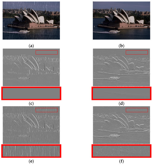
Figure 1.
(a,b) are the rainy image and rainless image, respectively. (c,d) are the gradient maps of the rainless image along the x and y directions, respectively. (e,f) are the gradient maps of corresponding rainy image along the x and y directions, respectively.
On the basis of the above analysis, aiming at the sparsity of gradient information in the y-direction, we directly construct a prior constraint to constrain the rain layer by using the y-direction gradient of the rain layer as the third regularization term in Equation (4). Considering the influence of the scene depth, the width of the rain streaks is different. Therefore, to better detect the rain streaks, we propose sparse coding based on multi-scale dictionaries to reconstruct the rain layer, which is employed to constrain the rain layer obtained in each iteration. If the rain layer obtained by each iteration is close to the sparse reconstructed rain layer, then the x-direction gradient of the difference between these two rain layers is sparse. In other words, the rain streaks detected in the main direction of rain falling is more accurate. Therefore, we construct an x-direction gradient sparse prior regulation term to constrain the rain layer by using a sparse reconstruction rain layer in each iteration as the fourth regularization term in Equation (4).
At the same time, the coefficients of the convolution sparse coding are constrained to ensure their sparsity as the fifth term in Equation (4). To solve the model more accurately, the singular value decomposition (SVD) is used to initialize multi-scale dictionaries for the sparse coding. The initialization of multi-scale dictionaries is described in detail below. During the process of solving the rain layer and the background layer, the multi-scale dictionaries will be updated concurrently.
3.2.2. Initialization of Multi-Scale Dictionaries
Considering the size difference of raindrops or rain streaks in rain images, we propose the sparse coding based on multi-scale dictionaries to reconstruct a rain layer and constrain the layer solved in each iteration. In this paper, we define the multi-scale dictionaries with different sizes (15 × 15, 11 × 11, 7 × 7, and 3 × 3), which can be regarded as convolution filters to extract the information of the rain streaks with different sizes. The multi-scale dictionaries are first constructed by utilizing the initial rain layer, and then updated to encode the rain layer during each iteration. The initialization procedures of the dictionaries are described as follows:
- Input the initial rain layer R and define a dictionary template with size K, which is the identity matrix of (15 × 15, 11 × 11, 7 × 7, and 3 × 3).
- The rain layer is divided into many patches with a size of 15 × 15, and the step size is 1. Then, the average value of each block is calculated, and the difference blocks are obtained by subtracting the average value from the pixel values of each block.
- The difference blocks are reshaped into the column vectors, and the column vectors of the blocks are multiplied by their transposed vectors to obtain matrices with a size of 225 × 225.
- SVD is applied to the matrices obtained in (3) to extract the decomposed components and initialize the four dictionaries. Because rain streaks generally have the brightest intensities and their values are nonnegative, we extract the nonnegative data of the first K column vectors as the values of the dictionaries and then import the values into the dictionary template.
3.2.3. Solution for the Proposed Model
In the process of solving the rain removal model, it is necessary to provide a priori supplementary information for the model, such as and in Equation (3), which are used to regularize the two separation layers: the background layer and the rain layer, respectively. The rain removal model defined in this paper is shown in Equation (4), which is solved by the alternating iteration method to obtain the accurate rain layer and the background layer. To solve the model (4), we need to decompose the rain image into the initial rain layer and background layer (no rain layer). The process is described as follows. First, by considering that the main direction of rain streaks is mainly vertical and reflected in the horizontal gradient, two horizontal gradient filters are selected as second-order gradient operators to filter the rain image to obtain the background layer (i.e., the rainless image). Then, the initial rain layer is obtained by subtracting the background layer from the rain image and then employed to initialize the multi-scale dictionaries. Next, ADMM method is utilized to update the dictionaries and coefficients of convolutional sparse coding as well as the background layer. The detailed procedure of the proposed method is described in Algorithm 1.
For the objective function in Equation (4), we rewrite the convolution in a multiplication form, and the new function has the following form:
where y, b, r, and mj are the vectorization of rain image Y, background layer B, rainy layer R, and feature map Mj, respectively. We define and as the corresponding block circulants with circulant block matrices of filters and , and the solution details of the two variable sub-problems are as follows.
| Algorithm 1 Pseudocode of Single Image Rain Removal Based on Multi-scale Dictionary Learning |
| Initialization: Rain image Y and regularization parameter. Output: Background image B and rain layer R. Initialize multi-scale dictionaries by filtering the input rain image; Outer loop: iteration t = 1 to T 1. Update the background image bk by convolutional coding of the two horizontal filters by Equation (9); 2. Inner loop (update the rain layer R): for each iteration j = 1 to J do (a) Update the sparse coding by Equation (15) using ADMM operation; (b) The obtained and learned multiple dictionaries are used to solve the sparse reconstruction of ; (c) Update the constrained rain layer using Equation (18); 3. Update the multi-scale dictionary through a sparse coefficient and rain layer image using Equation (12). |
Subproblem
Two horizontal gradient filters are used as a sparse dictionary during the convolution sparse coding for the background layer, which can be solved by adding a prior term [14]. The initialization of the rain layer R0 = 0 is a fixed r to solve the algorithm as follows:
During the background layer optimization, we set x = y − r as a fixed value and introduce the group of auxiliary variables . The problem in (6) can be expressed as:
We then use the augmented Lagrangian function to solve problem (7) as follows:
The solution to each variable is solved using ADMM, as shown below:
where Li is the Lagrange variable for si, and and are the parameters in the algorithm. We set and empirically, where denotes a soft-thresholding operator with parameter . The closed solution of (7) is efficiently solved by (9).
Subproblem
The solution to r requires the value of the intermediate variables FR, j and mj. Therefore, we create F = [FR1, FR2,…, FRM] and as two matrices. The optimization problem with respect to r is rewritten as follows:
For Equation (10), we first need to calculate the values of F and M, setting . The solution to Equation (10) can be obtained by using the Lagrange algorithm as follows:
We adopt the ADMM scheme and exploit the FFT to improve the computation efficiency. The solution to each variable is as follows:
where r is a constant, and p1 is a Lagrange variable; thus, we need to optimize the convolutional sparsity coefficient M as follows:
The subproblems of M are solved using a lasso regression [38], and we set up the intermediate variables: . The optimization problem of M is then transformed into the following:
where c is a constant, and the optimized M is obtained by the soft threshold algorithm as follows:
Finally, by fixing b, mj, and FR, j, we solve the following sub-problem to obtain r:
Here, we set z = y − b as a fixed value, and introduce a group of auxiliary variables to solve problem (16), and the augmented Lagrangian form of r can be written as follows:
The constrained rain layer r can be solved by the Lagrangian algorithm:
4. Experiments
4.1. Datasets
To verify the effectiveness of the proposed method, the corresponding experiments are carried out on the simulated and real rain images. The specific arrangement of this section is organized as follows. First, the experimental environment and datasets are introduced. Then, through an analysis of the experimental results on the Rain 12 dataset [14], the parameters in the proposed model are determined. Finally, the proposed method is compared with some state-of-the-art methods, including GF [16], GMM [12], JCAS [14], DetailsNet [26], and LPNet [28]. To better show the effect of the methods, we selected 10 simulated images (as shown in Figure 2) and 2 real images to evaluate the performance of all methods. The effects of all the comparison methods were verified in terms of objective indexes and subjective vision.
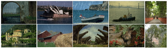
Figure 2.
Ten test images in our experiments.
4.2. Experimental Setup
The proposed method, GF [16], GMM [12], and JCAS [14] are run in MATLAB 2018a on computers with a 2.60 GHz Intel(R) Core (TM) i5–4210 m. Two deep-learning methods (DetailsNet [26] and LPNet [28]) are implemented in Pytorch and trained on NVDIA GTX 1080Ti GPUs. During the experiments, all the datasets and source codes of the comparison methods are derived from the original authors.
4.3. Experimental Parameters
4.3.1. Number of Iterations
Although an increase in the number of iterations will improve the experimental results, the computational cost should be considered during the actual operation.
To determine the appropriate iteration parameters, we employ the proposed method on the Rain 12 dataset to obtain the average objective evaluation indexes and the execution times under different numbers of iterations. The experimental results are shown in Figure 3, which shows a line chart of the average PSNR, SSIM values, and running time of test code (in seconds) as the number of iterations increases. The abscissa represents the number of iterations, and the ordinate indicates the changes in the curve of the PSNR values, SSIM values, and running time of test code. The results of 24 iterations are recorded during this experiment, and the average time of each iteration is approximately 50 s. To better display the experimental data and compare their differences, we reduce the obtained average PSNR, SSIM values, and the running time, and only mark certain indicators (the SSIM is the original value, the PSNR value is reduced by 100-fold, and the running time is reduced by 1000-fold). As can be seen from Figure 3, when the number of iterations is 19, the average values of the PSNR and SSIM reach the maximum values, which are only 0.001 dB and 0.0007 higher than the average values for 14 iterations, whereas the time consumed increases by nearly 240 s. Therefore, considering the computational cost, we finally choose T = 14 iterations.
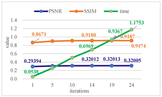
Figure 3.
The average PSNR, SSIM values, and running time on the Rain 12 dataset in the experiment increased with the number of iterations.
4.3.2. Regularization Parameter
Four regularization parameters exist in the proposed rain removal model, in which α is used to limit the sparsity constraint on the background layer, and limit two gradient prior terms, and is used to limit the convolutional sparse coding coefficient for the rain layer.
In the experiments, we limit the values of α and to [0.001, 0.01] and [0.001, 0.12], respectively. By self-adapting the values of and , and are sampled at intervals of 0.001 and 0.002, respectively, that is, α = [0.001, 0.001, 0.01] and = [0.001, 0.002, 0.012]. Different combinations of α and are used in the model to test the Rain 12 dataset. The average PSNR and SSIM values of the rain removal results are shown in Figure 4 (the marked values of α and on the coordinate axis are enlarged by 1000 times for convenience). From Figure 4, it can be seen that the values of α and have a significant influence on the experiment results, and combined with the extremum points of the PSNR and SSIM, we finally choose α = 0.005 and .
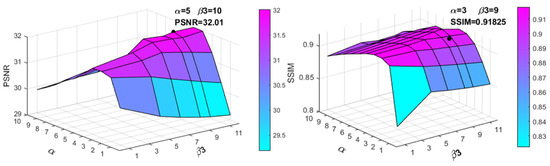
Figure 4.
The average PSNR and SSIM of the 12 images in the experiment increased with α and respectively on the exponential function.
Here, and are used to limit the gradient sparse prior terms, which constrain the reconstruction of the rain layer by using the horizontal and vertical gradient information of the rain layer. When the information of the rain layer is more abundant, the gradient value of the rain layer will be larger. Therefore, we think that the more abundant the rain layer information is, the stronger the constraint of the gradient sparse prior terms should be. On the basis of this consideration, this paper defines and as monotone increasing functions of and , and thus and can be adaptively determined on the basis of the intensity of the rainfall gradient information. In the experiments, we define two exponential functions to obtain the values of and . The definitions of and are as follows: and , where is a small constant. For these two definitions, we also carried out experiments on the Rain 12 dataset to determine the choice of α0 = 0.004 according to the average PSNR value, as shown in Figure 5.
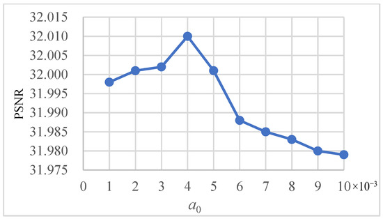
Figure 5.
The average PSNR of different values on the exponential function.
4.4. Experiments on Simulated Sets
To compare these methods fairly, 10 test images are selected from the published dataset [14], which are widely accepted and used by most researchers engaged in image rain removal.
To prove the validity of the sparse directional gradient regularization terms proposed in this paper, we carried out ablation experiments for different models to obtain the rain removal results. The objective indexes of the results of the different models are shown in Table 1. In Table 1, the original model contains only the first and second items of Equation (4), namely Model 1. Model 2 indicates that two gradient priors, and , are added to the original model. Model 3 is a model that removes two gradient priors on the basis of Formula (4) and utilizes multiscale dictionaries to reconstruct the rain layer in the model. Our model refers to the model of Equation (4). The four groups of data in Table 1 represent the average values of the PSNR and SSIM of the rain removal results obtained by executing four models on the 10 test images. It can be seen from Table 1 that the PSNR and SSIM values obtained by Model 2 with a gradient prior and Model 3 with multi-scale dictionaries are higher than those obtained by the original model. Our model with two gradient priors and multi-scale dictionaries achieves the highest evaluation indexes in all the models. As a result, our model can obtain better rain removal results.

Table 1.
PSNR (dB)/SSIM Results of Images after Rain Removal by Different Models.
To further evaluate the performance of the proposed model, we illustrate the average values of the PSNR and SSIM of the rain removal results obtained through various comparison methods on 10 test images, as shown in Table 2. The best indicators are marked in red and bold, and the second-best indicators are underlined. As can be seen from Table 2, the proposed algorithm in this study obtains the highest average PSNR and SSIM values. Compared with the other methods, the proposed method obtains higher PSNR and SSIM values on 10 test images, most of which are the highest and a few are the second highest. This shows that the proposed method is superior to the other comparison methods in terms of objective evaluation.
Table 2.
PSNR (dB)/SSIM Results of Images after Rain Removal by Different Methods.
The subjective effects of the synthetic experiments are shown in Figure 6 and Figure 7. Owing to the repeated use of guided filtering, the rain removal images obtained by the GF are more blurred and the details in the image are seriously lost. The results obtained by the GMM method still have residual information of the rain streaks and have the loss of the edge information. For example, there are obvious streaks in the sky area in Figure 6c, and Figure 7c also shows that the edges of the image are obviously blurred. Compared with the previous methods, the JCAS method retains more texture information of the original image and obtains a better rain removal image. However, there is still a small amount of rain streaks in the image, and there are also obvious artifacts, particularly in the high-frequency details of the image, such as the “bamboo” area in Figure 7e. The rain removal images obtained by DetailsNet, as shown in Figure 6f and Figure 7f, have a high structural similarity with the ground truth (rainless image), but there is also an obvious color distortion, such that the color of the image is brighter than that of the ground truth. The results obtained by the LPNet method have obvious noise and artifacts, and the structural details of the image are lost, as can be observed in Figure 7g. Obviously, compared with other methods, the results obtained by the proposed algorithm retain more structural details, have a more realistic visual effect, and are closer to the ground truth.
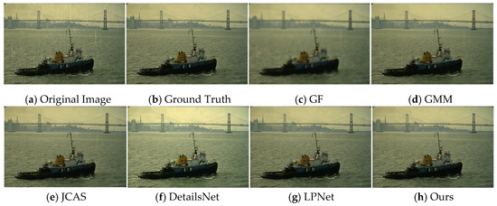
Figure 6.
The subjective visual effects of the synthetic image (“ship”) are compared in total. The first image is the synthetic rain image, the second image is the ground truth, and the following images are the results of GF, GMM, JCAS, DetailsNet, LPNet, and our method.
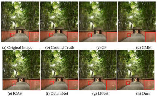
Figure 7.
The subjective visual effects of the synthetic image (“bamboo”) are compared in total. The first image is the synthetic rain image, the second image is the ground truth, and the following images are the results of GF, GMM, JCAS, DetailsNet, LPNet, and our method.
4.5. Experiments on Real Rainy Images
To verify the effectiveness of the proposed method in removing rain layers from real rain images, we tested various comparison methods for real rain images, and randomly selected two images to display the experimental results, as shown in Figure 8 and Figure 9. To better observe the results of the rain removal results, we select a small area in the image to enlarge to compare the details of the image. It can be seen from Figure 8 and Figure 9 that the traditional methods, such as the proposed method and the JCAS method, obtain better results for real rain images. Because of the neglect of the difference between the synthetic training set and the real rain images, the algorithms based on deep learning, such as DetailsNet and LPNet, cannot remove the rain streaks thoroughly. For example, in the enlarged areas of Figure 8e,f and Figure 9e,f, the residual rain streaks can be clearly observed. To solve the difference between the synthetic training set and the real rain images, real-time training of the proposed multi-scale dictionaries is employed to detect the information of the rain streaks in this study. From Figure 8g and Figure 9g, it can be seen that our method can obtain better rain remove results with less rain streaks.
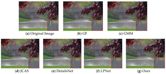
Figure 8.
The subjective visual effects of real image are compared in total. The first image is the input image, and the following images are the results of GF, GMM, JCAS, DetailsNet, LPNet and our method.
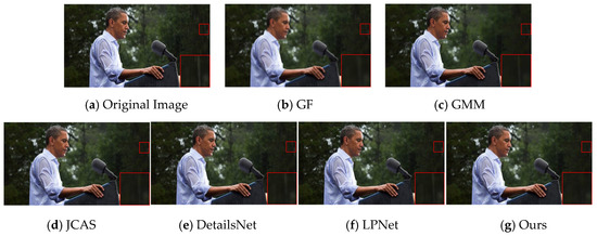
Figure 9.
The subjective visual effects of real image (“Obama”) are compared in total. The first image is the input image, and the following images are the results of GF, GMM, JCAS, DetailsNet, LPNet, and our method.
5. Conclusions
In this paper, a rain removal model based on directional gradient priors is constructed. First, to extract the refined rain layer, the x-direction and y-direction gradient sparse prior terms used to constrain the rain layer are proposed. Then, for the x-direction gradient sparse constraint, a multi-scale dictionary is constructed and updated in real time to detect rain streaks and sparse coding rain layers. Finally, the ADMM method is used to solve the proposed rain removal model to obtain the background layer and rain layer of the rain image alternately. The experimental results also show that the algorithm proposed in this paper can remove the rain streaks in the rain image and retain the structural information of the original rain image to the maximum extent possible. Compared with some other popular methods, the proposed method achieves better results both subjectively and objectively. In practical applications, owing to the uncertain factors caused by the rain environment, the images taken in a real rain scene may be affected by fog and various types of noise. Therefore, there remain areas of development for single image rain removal. Future research should focus on real scene images of rainy days, particularly when considering the influence of rainstorms, which will be helpful for the recognition and detection of outdoor computer vision systems used on rainy days.
Author Contributions
Conceptualization, S.H., Y.X. and Y.Y.; methodology, S.H.; software, Y.X. and M.R.; validation, Y.X., M.R. and W.W.; formal analysis, W.W. and M.R.; investigation, S.H. and Y.Y.; resources, Y.X.; data curation, Y.X.; writing—original draft preparation, S.H. and Y.X.; writing—review and editing, S.H., Y.X. and Y.Y.; visualization, Y.X. and W.W.; supervision, S.H. and Y.Y.; project administration, S.H. and Y.Y. All authors have read and agreed to the published version of the manuscript.
Funding
This research was funded by the National Natural Science Foundation of China (No. 61862030 and No. 62261025), by the Natural Science Foundation of Jiangxi Province (No. 20192ACB20002 and No. 20192ACBL21008), and by the Talent project of Jiangxi Thousand Talents Program (No. jxsq2019201056).
Conflicts of Interest
The authors declare no conflict of interest.
References
- Bossu, J.; Hautière, N.; Tarel, J.P. Rain or snow detection in image sequences through use of a histogram of orientation of streaks. Int. J. Comput. Vis. 2011, 93, 348–367. [Google Scholar] [CrossRef]
- Tripathi, A.K.; Mukhopadhyay, S. Meteorological approach for detection and removal of rain from videos. IET Comput. Vis. 2013, 7, 36–47. [Google Scholar] [CrossRef]
- Barnum, P.C.; Narasimhan, S.; Kanade, T. Analysis of rain and snow in frequency space. Int. J. Comput. Vis. 2010, 86, 256–274. [Google Scholar] [CrossRef]
- Yan, W.; Tan, R.T.; Yang, W.; Dai, D. Self-Aligned Video Deraining with Transmission-Depth Consistency. In Proceedings of the IEEE Conference on Computer Vision and Pattern Recognition, Nashville, TN, USA, 20–25 June 2021; pp. 11966–11976. [Google Scholar]
- Ren, W.; Tian, J.; Han, Z.; Chan, A.; Tang, Y. Video desnowing and deraining based on matrix decomposition. In Proceedings of the IEEE Conference on Computer Vision and Pattern Recognition, Honolulu, HI, USA, 21–26 July 2017; pp. 2838–2847. [Google Scholar]
- Li, M.; Cao, X.; Zhao, Q.; Zhang, L.; Gao, C.; Meng, D. Video rain/snow removal by transformed online multiscale convolutional sparse coding. arXiv 2019, arXiv:1909.06148. [Google Scholar]
- Chao, R.; He, X.; Nguyen, T.Q. D3R-Net: Dynamic routing residue recurrent network for video rain removal. IEEE Trans. Image Process. 2019, 28, 699–712. [Google Scholar]
- Chen, J.; Tan, C.; Hou, J.; Chau, L.; Li, H. Robust video content alignment and compensation for rain removal in a CNN framework. In Proceedings of the IEEE Conference on Computer Vision and Pattern Recognition, Salt Lake City, UT, USA, 18–23 June 2018; pp. 6286–6295. [Google Scholar]
- Kang, L.; Lin, C.; Fu, Y. Automatic single-image-based rain streaks removal via image decomposition. IEEE Trans. Image Process. 2012, 21, 1742–1755. [Google Scholar] [CrossRef] [PubMed]
- Chen, D.; Chen, C.; Kang, L. Visual depth guided color image rain streaks removal using sparse coding. IEEE Trans. Circuits Syst. Video Technol. 2014, 24, 1430–1455. [Google Scholar] [CrossRef]
- Luo, Y.; Xu, Y.; Ji, H. Removing rain from a single image via discriminative sparse coding. In Proceedings of the IEEE International Conference on Computer Vision (ICCV), Santiago, Chile, 7–13 December 2015; pp. 3397–3405. [Google Scholar]
- Li, Y.; Tan, R.; Guo, X.; Lu, J.; Brown, M.S. Rain streak removal using layer priors. In Proceedings of the IEEE Conference on Computer Vision and Pattern Recognition, Las Vegas, NV, USA, 27–30 June 2016; pp. 2736–2744. [Google Scholar]
- Wang, Y.; Liu, S.; Xie, D.; Zeng, B. Removing rain streaks by a linear model. IEEE Access. 2020, 8, 54802–54815. [Google Scholar] [CrossRef]
- Gu, S.; Meng, D.; Zuo, W.; Zhang, L. Joint convolutional analysis and synthesis sparse representation for single image layer separation. In Proceedings of the IEEE International Conference on Computer Vision (ICCV), Venice, Italy, 22–29 October 2017; pp. 1717–1725. [Google Scholar]
- Wang, Y.; Liu, S.; Chen, C.; Zeng, B. A hierarchical approach for rain or snow removing in a single color image. IEEE Trans. Image Process. 2017, 26, 3936–3950. [Google Scholar] [CrossRef] [PubMed]
- Xu, J.; Zhao, W.; Liu, P.; Tang, X. Removing rain and snow in a single image using guided filter. In Proceedings of the IEEE International Conference on Computer Science and Automation Engineering (CSAE), Zhangjiajie, China, 25–27 May 2012; pp. 304–307. [Google Scholar]
- Zheng, X.; Liao, Y.; Guo, W.; Fu, X.; Ding, X. Single-image-based rain and snow removal using multi-guided filter. In Neural Information Processing, Proceedings of the 20th International Conference, ICONIP 2013, Daegu, Korea, 3–7 November 2013; Springer: Berlin/Heidelberg, Germany, 2013; pp. 258–265. [Google Scholar]
- Ding, X.; Chen, L.; Zheng, X.; Huang, Y.; Zeng, D. Single image rain and snow removal via guided L0 smoothing filter. Multimed. Tools Appl. 2016, 75, 2697–2712. [Google Scholar] [CrossRef]
- Kumar, D.; Kukreja, V. N-CNN Based Transfer Learning Method for Classification of Powdery Mildew Wheat Disease. In Proceedings of the International Conference on Emerging Smart Computing and Informatics (ESCI), Pune, India, 5–7 March 2021; pp. 707–710. [Google Scholar]
- Kumar, D.; Kukreja, V. Deep learning in wheat diseases classification: A systematic review. Multimed. Tools Appl. 2022, 81, 10143–10187. [Google Scholar] [CrossRef]
- Kumar, D.; Kukreja, V. Automatic Classification of Wheat Rust Diseases Using Deep Convolutional Neural Networks. In Proceedings of the 9th International Conference on Reliability, Infocom Technologies and Optimization (Trends and Future Directions) (ICRITO), Noida, India, 3–4 September 2021; pp. 1–6. [Google Scholar]
- Kukreja, V.; Kumar, D.; Kaur, A. Deep learning in Human Gait Recognition: An Overview. In Proceedings of the International Conference on Advance Computing and Innovative Technologies in Engineering (ICACITE), Greater Noida, India, 4–5 March 2021; pp. 9–13. [Google Scholar]
- Kumar, D.; Kukreja, V. An Instance Segmentation Approach for Wheat Yellow Rust Disease Recognition. In Proceedings of the International Conference on Decision Aid Sciences and Application (DASA), Sakheer, Bahrain, 7–8 December 2021; pp. 926–931. [Google Scholar]
- Kumar, D.; Kukreja, V. Image-Based Wheat Mosaic Virus Detection with Mask-RCNN Model. In Proceedings of the International Conference on Decision Aid Sciences and Applications (DASA), Chiangrai, Thailand, 23–25 March 2022; pp. 178–182. [Google Scholar]
- Kumar, D.; Kukreja, V. Quantifying the Severity of Loose Smut in Wheat Using MRCNN. In Proceedings of the International Conference on Decision Aid Sciences and Applications (DASA), Chiangrai, Thailand, 23–25 March 2022; pp. 630–634. [Google Scholar]
- Fu, X.; Huang, J.; Zeng, D.; Huang, Y.; Ding, X.; Paisley, J. Removing rain from single images via a deep detail network. In Proceedings of the IEEE Conference on Computer Vision and Pattern Recognition, Honolulu, HI, USA, 21–26 July 2017; pp. 1097–1101. [Google Scholar]
- Zhang, H.; Patel, V.M. Density-aware single image de-raining using a multi-stream dense network. In Proceedings of the IEEE Conference on Computer Vision and Pattern Recognition, Salt Lake City, UT, USA, 18–23 June 2018; pp. 695–704. [Google Scholar]
- Fu, X.; Liang, B.; Huang, Y.; Ding, X.; Hu, Y.; Luk, K.D.K. Lightweight pyramid networks for image deraining. IEEE Trans. Neural Netw. Learn. Syst. 2020, 31, 1794–1807. [Google Scholar] [CrossRef] [PubMed]
- Hu, X.; Zhu, L.; Wang, T.; Fu, C.-W.; Heng, P.-A. Single-Image Real-Time Rain Removal Based on Depth-Guided Non-Local Features. IEEE Trans. Image Process. 2021, 30, 1759–1770. [Google Scholar] [CrossRef] [PubMed]
- Li, Y.; Brown, M.S. Single image layer separation using relative smoothness. In Proceedings of the IEEE Conference on Computer Vision and Pattern Recognition, Columbus, OH, USA, 23–28 June 2014; pp. 2752–2759. [Google Scholar]
- Jiang, T.; Huang, T.; Zhao, X.; Deng, L.; Wang, Y. FastDeRain: A novel video rain streak removal method using directional gradient priors. IEEE Trans. Image Process. 2019, 28, 2089–2102. [Google Scholar] [CrossRef] [PubMed]
- Li, X.; Orchard, M.T. New edge-directed interpolation. IEEE Trans. Image Process. 2001, 10, 1521–1527. [Google Scholar] [PubMed]
- Zhang, L.; Wu, X.L. An edge-guided image interpolation algorithm via directional filtering and data fusion. IEEE Trans. Image Process. 2006, 15, 2226–2238. [Google Scholar] [CrossRef] [PubMed]
- Gu, S.; Zuo, W.; Xie, Q.; Meng, D.; Feng, X.; Zhang, L. Convolutional sparse coding for image super-resolution. In Proceedings of the IEEE International Conference on Computer Vision (ICCV), Santiago, Chile, 7–13 December 2015; pp. 1823–1831. [Google Scholar]
- Gao, S.; Tsang, I.W.; Chia, L. Laplacian sparse coding, hypergraph laplacian sparse coding, and applications. IEEE Trans. Pattern Anal. Mach. Intell. 2013, 35, 92–104. [Google Scholar] [CrossRef] [PubMed]
- Bristow, H.; Eriksson, A.; Lucey, S. Fast convolutional sparse coding. In Proceedings of the IEEE Conference on Computer Vision and Pattern Recognition, Portland, OR, USA, 23–28 June 2013; pp. 391–398. [Google Scholar]
- Zhou, Y.; Chang, H.; Barner, K.; Spellman, P.; Parvin, B. Classification of histology sections via multispectral convolutional sparse coding. In Proceedings of the IEEE Conference on Computer Vision and Pattern Recognition, Columbus, OH, USA, 23–28 June 2014; pp. 3081–3088. [Google Scholar]
- Osendorfer, C.; Soyer, H.; van der Smagt, P. Image super-resolution with fast approximate convolutional sparse coding. In Neural Information Processing, Proceedings of the 21st International Conference, ICONIP 2014, Kuching, Malaysia, 3–6 November 2014; Springer: Cham, Switzerland, 2014; pp. 250–257. [Google Scholar]


Publisher’s Note: MDPI stays neutral with regard to jurisdictional claims in published maps and institutional affiliations. |
© 2022 by the authors. Licensee MDPI, Basel, Switzerland. This article is an open access article distributed under the terms and conditions of the Creative Commons Attribution (CC BY) license (https://creativecommons.org/licenses/by/4.0/).