The Use of a Movable Vehicle in a Stationary Condition for Indirect Bridge Damage Detection Using Baseline-Free Methodology

Abstract

The use of an instrumented scanning vehicle has become the center of focus for bridge health monitoring (BHM) due to its cost efficiency, mobility, and practicality. However, indirect BHM still faces challenges such as the effects of road roughness on vehicle response, which can be avoided when the vehicle is in a stationary condition. This paper proposes a baseline-free method to detect bridge damage using a stationary vehicle. The proposed method is implemented in three steps. First, the contact-point response (CPR) of the stationary vehicle is computed. Secondly, the CPR is decomposed into intrinsic mode functions (IMFs) using the variational mode decomposition (VMD) method. Finally, instantaneous amplitude (IA) of a high frequency IMF is computed. The peak represents the existence and location of the damage. A finite element model of a bridge with damage is created. The results show that the method can identify the damage location under different circumstances, such as a vehicle with and without damping, different speeds of the moving vehicle, different sizes of damage, and multiple damage. A higher speed was found to provide better visibility of damages. In addition, smaller damage was less visible than wider damage.

1. Introduction

Regular monitoring of bridges is crucial for bridge safety because it provides an early warning for authorities to take pre-emptive measures to avoid bridge collapse. Aging bridges, which make up a big portion of the current in-use bridges, pose a high risk of collapse because they are more susceptible to deterioration and damage [1]. Furthermore, the increasing traffic loads in the last decades have exceeded the intended design load capacity of those bridges [2]. Therefore, developing damage detection methods has become of a great concern to authorities and decision makers.

Vibration-based damage detection methods have been used extensively for bridge health monitoring (BHM). Bridge vibration signals carry useful information about the dynamic properties of the bridge. The change in dynamics properties of the bridge indicates structural damage and deterioration. Direct BHM requires each bridge to be equipped with a sensory system network of many accelerometers and date loggers in order to record the vibration data. Thereafter, the collected data go through signal processing to assess the health state of the bridge [3]. This method is called the direct method because the sensors are installed directly on the bridge. It is obvious how this method is costly and impractical to be used for the bridge network in a country [4]. Therefore, another method called the indirect method has been proposed to overcome the drawbacks of the direct method. The indirect method first emerged when Professor Yang YB proposed the use of an instrumented vehicle to record the bridge vibration [5]. They proved the feasibility of extracting bridge frequency using the scanning vehicle by theoretical derivation and finite element (FE) modelling. Soon after, Lin and Yang [6] proved the feasibility of extracting the bridge frequency from a moving vehicle in a field test. In the last two decades, the research focus of vibration-based BMH has been shifting towards indirect means that require only an instrumented vehicle to record the vibration signal of the bridge. It has been demonstrated that the indirect method is more effective and less costly than the direct method [7,8]. Plenty of research has been conducted to investigate the factors and challenges that are encountered when a vehicle is used to scan a bridge vibration. Analytical studies such as FE simulations and experimental studies such as laboratory and field tests have been widely used to study the indirect method.

Thorough review papers have been published discussing the accomplished progress of the indirect method [7,8,9]. Nevertheless, it is essential to view past research discussing the indirect method and the difficulties encountered when using the scanning vehicle. For example, in a field test experiment, Oshima, Yamaguchi [10] suggested using a heavy vehicle to obtain better visibility of the bridge frequency. Yang, Chang [11] proposed an advanced signal processing technique to detect higher modes of frequency of the bridge employing numerical simulation and field test experiments. González, O’brien [12] pointed out to the challenge of road roughness, which corrupts the recorded signal of the scanning vehicle. They proposed the use of data collected from accelerometers fixed on specific vehicle types to estimate the road roughness profile of the road. Kim, Isemoto [13] concluded that a higher vehicle speed would provide larger amplitude frequency peaks, but at the same time, a higher speed would provide low spectral accuracy due to road roughness. In fact, several studies have indicated the negative effects on the recorded signal of the scanning vehicle [8,9,14,15,16]. Yang, Li [17] proposed the subtraction of the acceleration spectra from two connected vehicles to remove or reduce the effects of road irregularities. Malekjafarian and O’Brien [18] proposed the use of frequency domain decomposition (FDD) as a more accurate alternative to fast Fourier transform (FFT) for bridge frequency identification in the presence of road roughness. In their review paper, Yang, Yang [9] emphasized the challenge by the road surface profile on the extraction of the bridge dynamic properties. They also highlighted the influence of the vehicle’s own frequency on the recorded signal by the vehicle. The vehicle’s own response could overshadow bridge vibration, which would misrepresent the dynamic properties of the bridge. Yang, Zhang [19] derived a formula to compute the contact-point response from the response of the scanning vehicle. They demonstrated that the contact-point response could eliminate the vehicle response, which pollutes the recorded signal. Although the contact-point response has provided a more accurate response for the bridge, it still does not solve the issue of road roughness. Yang, Xu [20] examined the use of the scanning vehicle in a stationary condition. They concluded that the stationary vehicle showed a higher mode of frequency and better visibility of bridge frequency than the vehicle in a moving condition. They mentioned that a stationary vehicle was not subjected to road roughness effects, thus providing better visibility than the moving vehicle. Hashlamon, Nikbakht [21] computed the contact-point response of a stationary vehicle in a numerical simulation study considering different scenarios. They demonstrated how the contact-point response of the stationary vehicle was almost identical to the bridge response taken form a fixed sensor on the bridge. As the scanning vehicle encounters road roughness challenge while passing over the bridge, it is advised that the scanning vehicle should be investigated while it is in a stationary position [22]. Therefore, this paper introduces the use of a vehicle in a stationary condition for damage detection. This paper suggests that when BHM is conducted using the scanning vehicle, not only should the vibration of the moving be used, but the vibration of the vehicle in a stationary condition should also be considered. This paper demonstrates how the scanning vehicle in a stationary position can be used for bridge damage detection.

When it comes to damage detection, bridge damage can be classified into four levels. The first level is the identification of damage existence, the second is determining the damage location, the third is determining the severity of the damage, and finally, estimating the remaining life service of the bridge [23]. The indirect method has been used extensively covering different levels of damage detection using a variety of methods. For example, Corbally, Malekjafarian [24] and Singh and Sadhu [25] used the scanning vehicle to detect the existence of bridge damage without determining the damage location. Meanwhile, ElHattab, Uddin [26] and Janeliukstis, Rucevskis [27] employed the indirect method to determine the damage and its location; however, they did not estimate the severity of the damage. Bandara, Rajeev [28] were also able to determine the damage location on the bridge using the scanning vehicle. They attempted to determine the severity of the damage, but they acknowledged that defect severity cannot be obtained by the proposed method. Other studies such as Kim, Isemoto [29] used a scale bridge model to examine the efficiency of using a scanning vehicle for damage detection in short span bridges. They managed to detect damage location and severity using a method that relies on prior information of the undamaged bridge. In fact, among the proposed methods, most of the techniques require baseline information about the healthy state of the bridge to be able to detect damages. However, prior information about most bridges is usually not available [30]. On the other hand, there are some proposed techniques that do not require prior information of the intact bridge, such methods are called baseline-free methods. Baseline-free methods are based on advanced signal processing techniques to identify damage without the need to refer to prior response of the healthy state bridge [31], where damage is often identified as irregularities or peaks at the damage location. In fact, signal processing techniques have been employed for baseline-based and baseline-free damage detection. For example, wavelet transform (WT) techniques have been widely used to detect damage while relying on prior information of the intact bridge [32,33,34]. Furthermore, OBrien, Malekjafarian [35] and Kildashti, Alamdari [36] used the empirical mode decomposition (EMD) technique for a baseline-based damage detection method. Zhang, Qian [37] and Yang, Zhang [38] proposed the use of instantaneous amplitude squared (IAS) for damage detection using a moving vehicle. Zhan, Au [39] proposed the use of contact point displacement difference (CPDD) for a baseline-free method. They found out that the proposed method was not able to detect damage near the boundary. However, when using a baseline-based method, such as coordinate modal assurance criterion (COMAC), damage at the boundary could be detected. This paper proposes the use of a series of advanced signal processing techniques to detect damage using a stationary vehicle, without relying on previous information of the intact bridge. The following section explains the proposed method in detail. Thereafter, a numerical simulation of a damaged bridge is presented. The proposed method is implemented to demonstrate how a vehicle in a stationary position can be used for bridge damage detection.

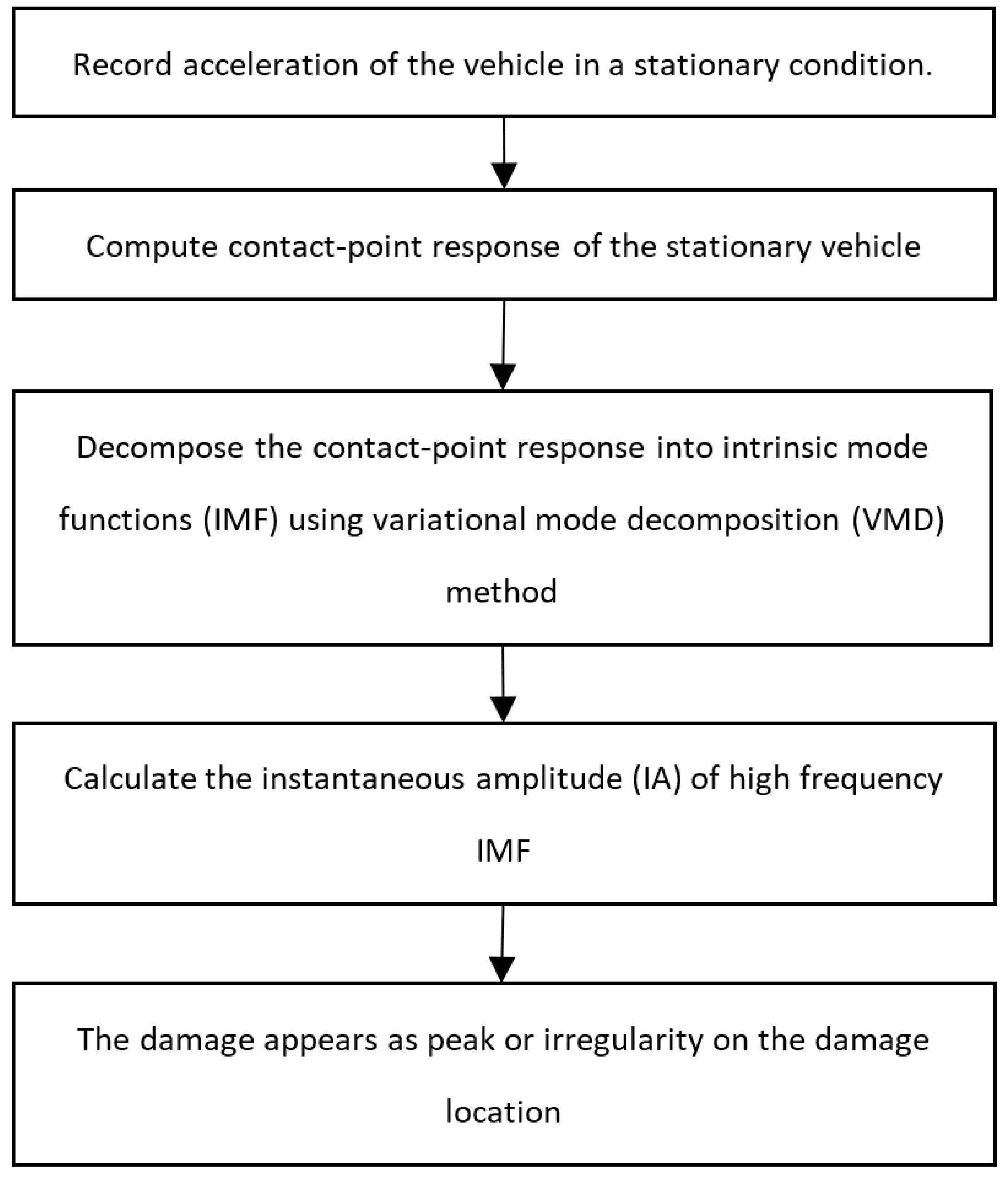
2. Damage Detection Using a Stationary Vehicle

This paper proposes a baseline-free method utilizing a set of advanced signal processing techniques to process the recorded vibration signal of a stationary vehicle. The first step in the proposed method is to eliminate vehicle’s own frequency, as the recorded signal contains both the bridge and vehicle vibration signals. By removing the vehicle’s own vibration, the obtained signal contains only the bridge’s vibration. This is done by computing the contact-point response of the stationary vehicle. Hashlamon, Nikbakht [21] have shown good agreement between the contact-point response and the bridge response under different circumstances. In the second step, the contact-point response is decomposed into different mono-component signals, which reflect the state of the bridge. A new technique was recently proposed, called the variational mode decomposition (VMD), which has shown good outcomes in decomposing time series signals. Finally, instantaneous frequency (IA) is computed for high frequency signals to show the damage as irregularities or as peaks at the damage location. Figure 1 shows the steps of the proposed method. The next sections elaborate, in detail, each step of the proposed method.

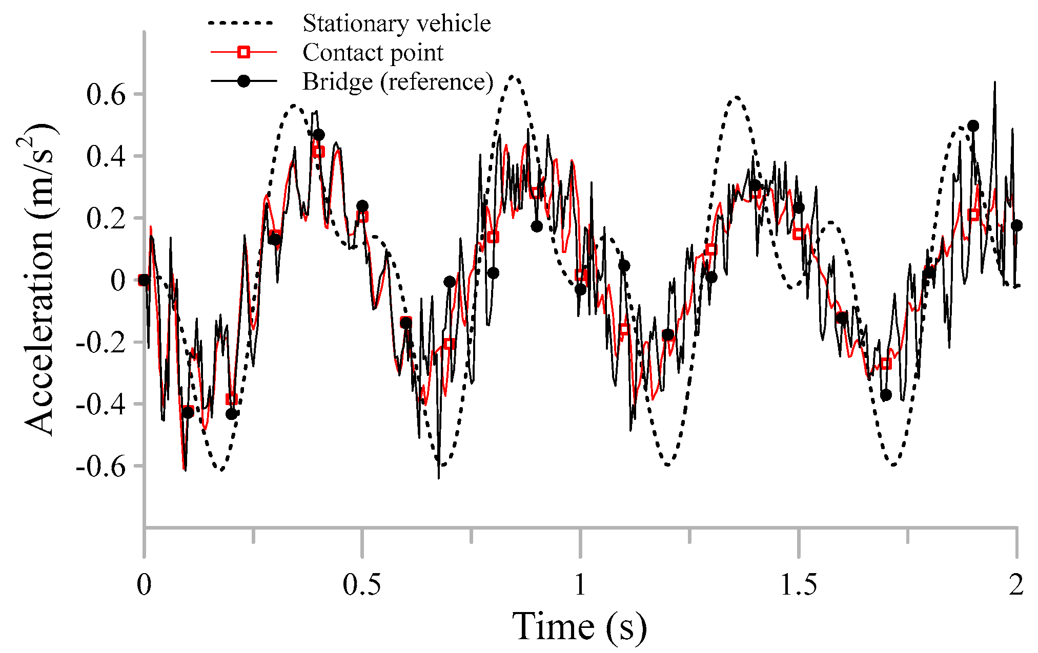
2.1. Contact-Point Response of the Stationary Vehicle

Indirect bridge vibration measurement is conducted by an accelerometer installed on a scanning vehicle that records the vertical vibration of the vehicle. The contact-point response of the scanning vehicle refers to the response of the point below the vehicle’s tire, which is in direct contact with the bridge. By calculating the contact-point response, the vehicle’s frequency can be eliminated, which would provide a more accurate representation of the bridge response. Yang, Zhang [19] provided a technique to extract the contact-point response from the vibration signal recorded by a moving vehicle. The same technique could be applied for a stationary vehicle vibration response. Figure 2 shows a stationary vehicle parked at mid-span, where another moving vehicle passes over the bridge as a source of excitation.

The equation of motion of the stationary vehicle can be expressed in terms of the contact-point displacement response $u_c$, as the following:

$$m_s{\ddot{q}}_s+k_s\left(q_s-u_c\right)=0$$

(1)

where $m_s$ and $k_s$ are the mass and stiffness of the stationary vehicle, respectively. ${\ddot{q}}_s$ and $q_s$ are the acceleration and displacement responses of the stationary vehicle, respectively. Equation (1) is derived twice with respect to time to obtain Equation (2). By rearranging Equation (2), the contact-point response can be calculated as shown in Equation (3).

$$k_s\left({\ddot{q}}_s-{\ddot{u}}_c\right)=m_s\frac{d^2{\ddot{q}}_s}{d{t}^2}$$

(2)

$${\ddot{u}}_c={\ddot{q}}_s+\frac{d^2{\ddot{q}}_s}{{\omega }_s^{2}d{t}^2}$$

(3)

${\omega }_s$ is the stationary vehicle natural frequency and ${\ddot{u}}_c$ is the contact-point acceleration response. In practice, ${\ddot{q}}_s$ is the recorded signal by the vehicle and ${\omega }_s$ can be measured or calculated. Finally, the term $\frac{d^2{\ddot{q}}_s}{d{t}^2}$ can be calculated by the central difference method for the discrete data of the recorded signal as shown in Equation (4), where $\mathsf{\Delta }t$ is the sampling interval and i denotes the ith sampling point.

$$\frac{d^2{\ddot{q}}_s}{d{t}^2}=\frac{\left({\ddot{q}}_s{|}_{i+1}-2{\ddot{q}}_s{|}_i+{\ddot{q}}_s{|}_{i-1}\right)}{{(\mathsf{\Delta }t)}^2}$$

(4)

2.2. Decomposition of Contact-Point Response

The vibration signal of the bridge carries information about the bridge properties that contain damage indications. To separate the contact-point response into several meaningful mono-component signals, several techniques could be used. Empirical mode decomposition (EMD) has been used widely for structural damage detection to decompose the vibration signal of the structure [30]. EMD is an innovative technique that has been proposed as part of the Hilbert Huang transform (HHT), which is able to preserve the nonlinear response of the bridge at the damage location [31,40]. EMD decomposes the signal into several mono-component signals called intrinsic mode functions (IMFs). The first IMF contains a higher frequency signal, which contains damage information, which is usually used for damage detection [41,42,43]. The nonlinear effects of structure damage have the tendency to be of higher frequencies. Therefore, higher frequency bands are more likely to contain the damage information. Meredith, González [43] proposed a damage detection technique employing EMD to detect multiple damage in a simple-beam bridge. However, the road roughness of the bridge is not considered in their study. OBrien, Malekjafarian [35] proposed an indirect damage detection technique based on EMD while considering the road roughness effects. However, the proposed method relies on subtracting the difference of the IMFs from damage and healthy signals (baseline-based technique). Therefore, it is necessary to have prior information of the intact bridge to implement the method. In general, most damage detection EMD-based studies employ baseline-based methods that require a prior response of the undamaged bridge [31]. In addition, EMD is an empirical method; being empirical, it fails sometimes to decompose the non-stationary signal into perfectly narrow-banded mono-component signals.

Recently, Dragomiretskiy and Zosso [44] introduced a new method, called variational mode decomposition (VMD), to deal with the limitations of the EMD method. The VMD is fundamentally different from the recursive EMD as it preforms adaptive decomposition of the signal into its components [44]. VMD has shown a superior performance in decomposing non-stationary signals over the EMD method [31,44]. The method is a generalization of the classic Wiener filter. The main algorithm and MATLAB code of the VMD method can be found in Dragomiretskiy and Zosso’s original paper [44]. The number of IMFs in the VMD method can be controlled, unlike in the EMD method. The ideal number of modes depends on the knowledge of physics of the non-stationary signal. Therefore, in this paper, VMD will be used for signal decomposition of the contact-point response for identifying damage locations.

2.3. Instantaneous Amplitude of High Frequency IMF

Hilbert transform (HT) is known to be used for exposing the instantaneous attributes of time-domain signals. The envelope of a time signal, which is known as the instantaneous amplitude (IA), shows the discontinuity of the signal, which indicates the location of the damage. Therefore, when the contact-point signal is decomposed into several IMFs, the IA of the high frequency signal is computed.

The HT of a signal s(t) is defined as its convolution with a unit impulse function of 1/πt, as shown in Equation (5). The two signals s(t) and h(t) that form the analytical function z(t) are shown in Equation (6). Where A(t) represents the instantaneous amplitude (IA) and ϴ(t) is the instantaneous phase.

$$h(t)=H\left[s\left(t\right)\right]=\frac{1}{\pi }{{\displaystyle \int }}_{-\infty }^{\infty }\frac{s\left(\tau \right)}{t-\tau }d\tau$$

(5)

$$z(t)=s\left(t\right)+ih\left(t\right)=A\left(t\right)e^{i\theta \left(t\right)}$$

(6)

IA is the envelope of the original signal, and it varies with time. These parameters of the instantaneous phase and amplitude are physically meaningful when the signal is mono-component or narrow-banded as the IMFs that are obtained by the VMD method. IA is computed as follows:

$$A(t)=\pm \sqrt{{\left[s\left(t\right)\right]}^2+{\left[h\left(t\right)\right]}^2}$$

(7)

3. Finite Element Modulation and Damage Detection

In this section, the proposed damage detection method is implemented on a stationary vehicle response obtained from a FE model. The FE consists of 2D bridge made of shell elements in the commercial program of Ls-Dyna. Properties of the bridge are taken from the study of Yang, Lin [5] which are shown in

Table 1. Beam Properties.

Property	Value
Bridge length	25 m
Elastic modulus	27.5 GN/m2
Moment of inertia	0.12 m4
Bridge length density	4800 kg/m

. The FE bridge model is divided equally into 1000 shell elements. Each element is of 0.25 m of length and 0.2357 m of width. The moving vehicle is modelled as a quarter car of two degrees of freedom, while the stationary vehicle is parked on the bridge and modelled as quarter car of single degree of freedom. The properties of the moving and stationary vehicles are shown in

Table 2. Properties of the moving and stationary vehicles.

Property	Value
Stationary vehicle body mass	200 kg
Stationary vehicle spring stiffness	1.2 × 105 N/m
Stationary vehicle frequency	3.98 Hz
Moving vehicle body mass	14,000 kg
Moving vehicle axle mass	1000 kg
Moving vehicle body stiffness	1.2 × 105 N/m
Moving vehicle axle stiffness	2000 N/m
Moving vehicle body damping	5%

. The moving vehicle starts moving for an approach distance of 75 m to remove the effects of vehicle translational vibration effects.

Road roughness is added in the FE model on the track where the moving vehicle is passing. Road roughness is simulated by the procedures introduced by ISO 8608 [45]. Road surface roughness can be obtained as follows:

$$r\left(x\right)={{\displaystyle \sum }}_i{d}_i\cos (n_{i}x+{\theta }_i)$$

(8)

$$d=\sqrt{2G_d(n)\mathsf{\Delta }n}$$

(9)

$$G_d\left(n\right)=G_d\left(n_0\right){\left(\frac{n}{n_0}\right)}^{-2}$$

(10)

where $n_0$ is a constant that is equal to 0.1 cycle/m. The road surface profile $G_d\left(n_0\right)$, in this paper is selected for class B of ISO standards, which is 6 × 10⁻⁶ m³. $\mathsf{\Delta }n$ represents the sampling interval for the spatial frequency, which is selected to be 0.04 cycle/m. The lower and upper spatial frequencies are selected as 1 and 100 cycle/m, respectively. Figure 3 shows the road surface profile of the class B roughness considering the mentioned values.

The stationary vehicle acceleration response is taken from the top node of the stationary single degree of the freedom vehicle model. Then, the contact-point response of the stationary vehicle is computed using Equations (3) and (4). It is worthy to note that the bridge response is different from the stationary vehicle response, which is demonstrated in Figure 4. However, it is also demonstrated that the contact-point response shows good agreement with the bridge response. Therefore, the stationary vehicle can be used as a movable accelerometer instead of fixing the accelerometer directly on the bridge following the conventional method, which has several disadvantages as mentioned earlier.

The damage on the bridge is modelled as stiffness reduction of shell elements of the bridge. Throughout this paper, the damage length is 1 m and the speed of the moving vehicle is 12.5 m/s, unless it is mentioned otherwise. The contact-point response of the stationary vehicle is decomposed into mono-component signals using the VMD method. Thereafter, the highest frequency mode is used to compute the IA.

3.1. Stationary Vehicle Location

The premise of the study is that the movable vehicle can be stationed at any location on the bridge. Therefore, the vehicle can be stationed at several locations until the damage existence and location are confirmed.

The first location of the vehicle is chosen to be at mid-span and the damage is located from 7.5 m to 8.5 m from the left side of the bridge. The IA of the high frequency IMF is shown in Figure 5. The IA amplitude shows irregularity around the stationary vehicle and damage locations. Irregularities around the stationary vehicle location occur because added mass is considered as damage [46]. Knowing where the car is parked, it noticed that the damage occurs around the point of 8 m from the left side of the bridge.

As there are some other minor irregularities such as between the vehicle at mid-span and the damage location, it is important to park the vehicle at different locations to examine the true location of the damage. Therefore, the movable vehicle is stationed now far from the damage, at 20 m from the left side of the bridge. Figure 6 shows the IA of the IMF of the stationary vehicle located far from the damage. It still shows irregularities around the vehicle and damage locations. This again indicates that the damage location is correctly identified at 8 m from the left side of the bridge.

When the vehicle is parked at mid-span (12.5 m away from the left side) and when it is located at 20 m away from the left side of the bridge, the IA results still show the correct location of the damage. Now, we have an idea where the location of the damage is. To further investigate the detection process, the vehicle is stationed at the detected damage location. Figure 7 shows the IA of the contact-point response of the vehicle when it is stationed at the damage location (8 m from the left side of the bridge). In this figure, there is only one peak, which is at the location of the damage and vehicle, unlike Figure 5 and Figure 6. This confirms the findings in Figure 5 and Figure 6.

Finally, although this method does not rely on previous information from the healthy bridge, it is worth showing what the IA of the healthy bridge would look like. Figure 8 compares the IA results of a stationary vehicle parked at mid-span from the damaged and undamaged bridges. It is noticed that for the healthy state bridge, the irregularities only occur at the vehicle location. It is important to note that irregularities happen at the end and beginning to the bridge due to the boundary conditions [39]. Therefore, even a healthy bridge would have irregularities at the boundaries of the bridge. This is considered one of the disadvantages of the proposed method. If the damage is near the boundary condition, it is difficult to detect such damage. The authors notice that from the beginning of the bridge until 6 m, the irregularities do not represent damage, but the boundary condition of the bridge.

3.2. Damped Vehicle

In this section, damping of 5% is added to the stationary vehicle. The procedure of the proposed method is applied on the damped stationary vehicle response. Figure 9 shows the IA of the IMF signal. There is a peak visible at the damage location when damping is added. However, the peak looks less visible when damping is considered.

3.3. Multiple Damages

This case study considers two points of damage on the bridge, with a second damage modelled from 18.5 to 19.5 m on the bridge. The procedure is applied again on the stationary vehicle acceleration response. The IA of high IMF in Figure 10 shows the two forms of damage clearly as peaks at the locations of the damage. The stationary vehicle is also shown as a peak in the middle of the bridge, that is because the added mass of the stationary vehicle is also considered as damage.

3.4. Smaller Damage

This section considers smaller damage of 0.5 m in length instead of 1 m in length. When the size of the damage is reduced, there is still a peak at the damage location, as shown in Figure 11; however, this peak is less significant than for the larger damage. This indicates that smaller damage might not be visible using the stationary vehicle. Nevertheless, the purpose of the proposed method in this paper is to introduce the concept of using the stationary vehicle as a means of damage detection.

3.5. Moving Vehicle Speed

A higher speed allows for more visibility of the damage in the bridge response [31]. In this section, the speed of the vehicle is reduced to 5 m/s to provide less excitation to the bridge so as to examine the proposed method. Figure 12 shows the IA of the high frequency IMF. It is shown that the peak due to the damage is still visible, despite the lower speed. It is noticed that the peak due to damage is less visible for lower speeds though.

4. Conclusions

This paper introduces the use of a vehicle in a stationary position to detect bridge damage. The proposed damage detection methodology is not based on a healthy bridge response baseline; therefore, it can detect damage without relying on prior information of the bridge. The method consists of three steps, which start by computing the contact-point response of the stationary vehicle, then decomposing the obtained response using VMD into narrow-banded IMFs, and finally, computing the IA of the high frequency IMF. While road roughness is considered, the method is examined under different conditions on a bridge of 25 m. The proposed method was implemented on bridge damage, considering several conditions such as the followings:

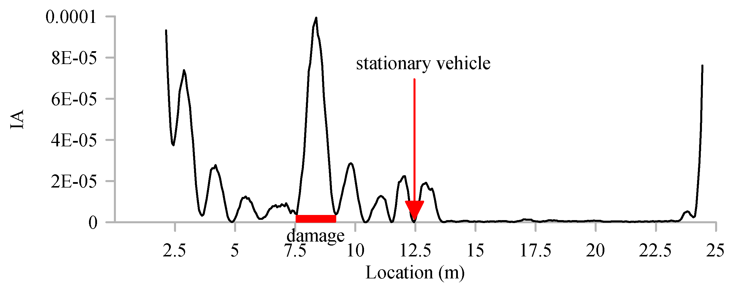
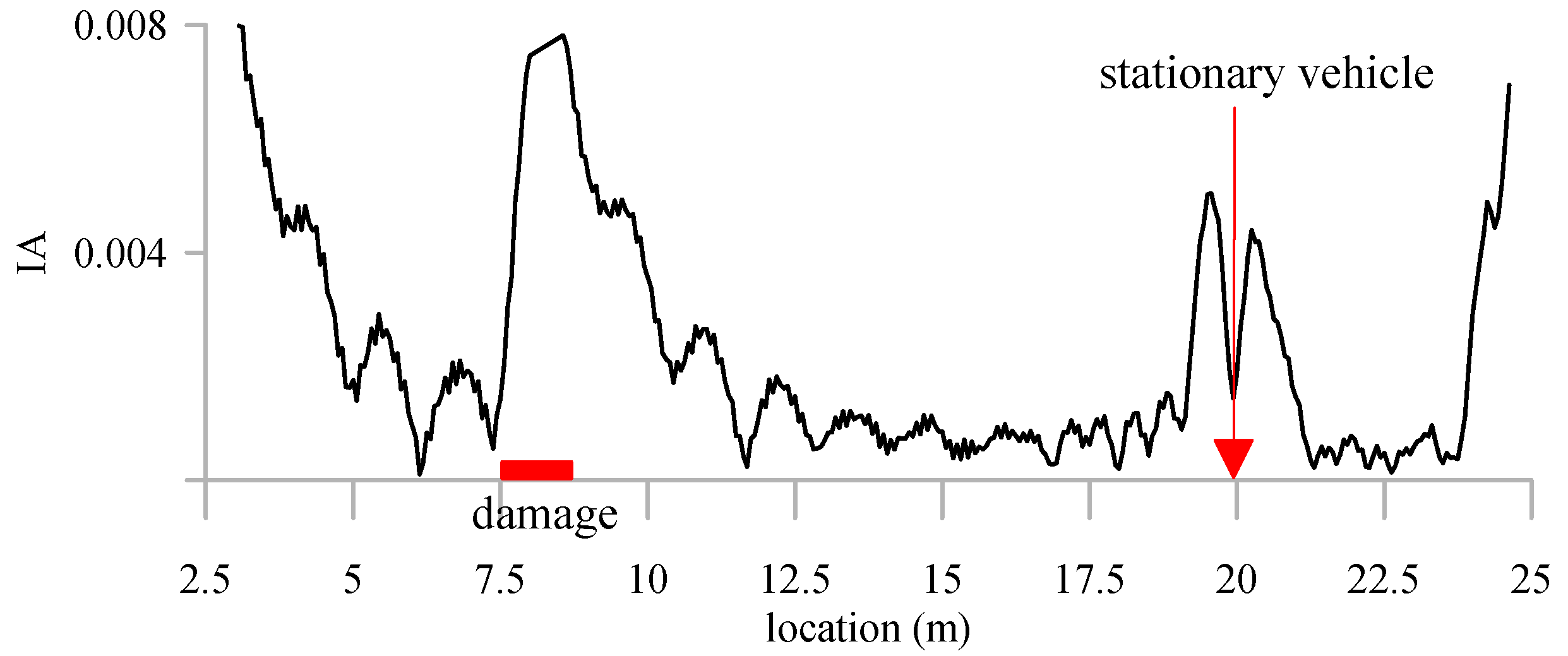
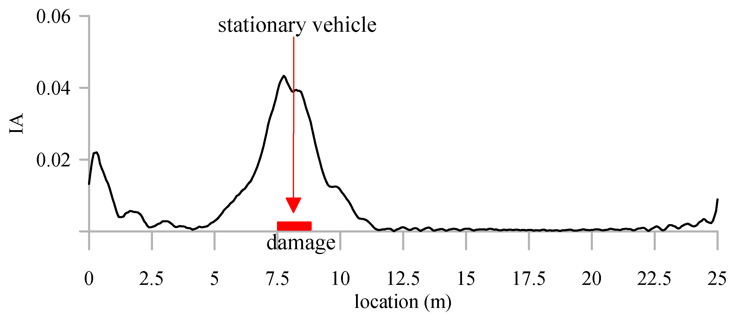
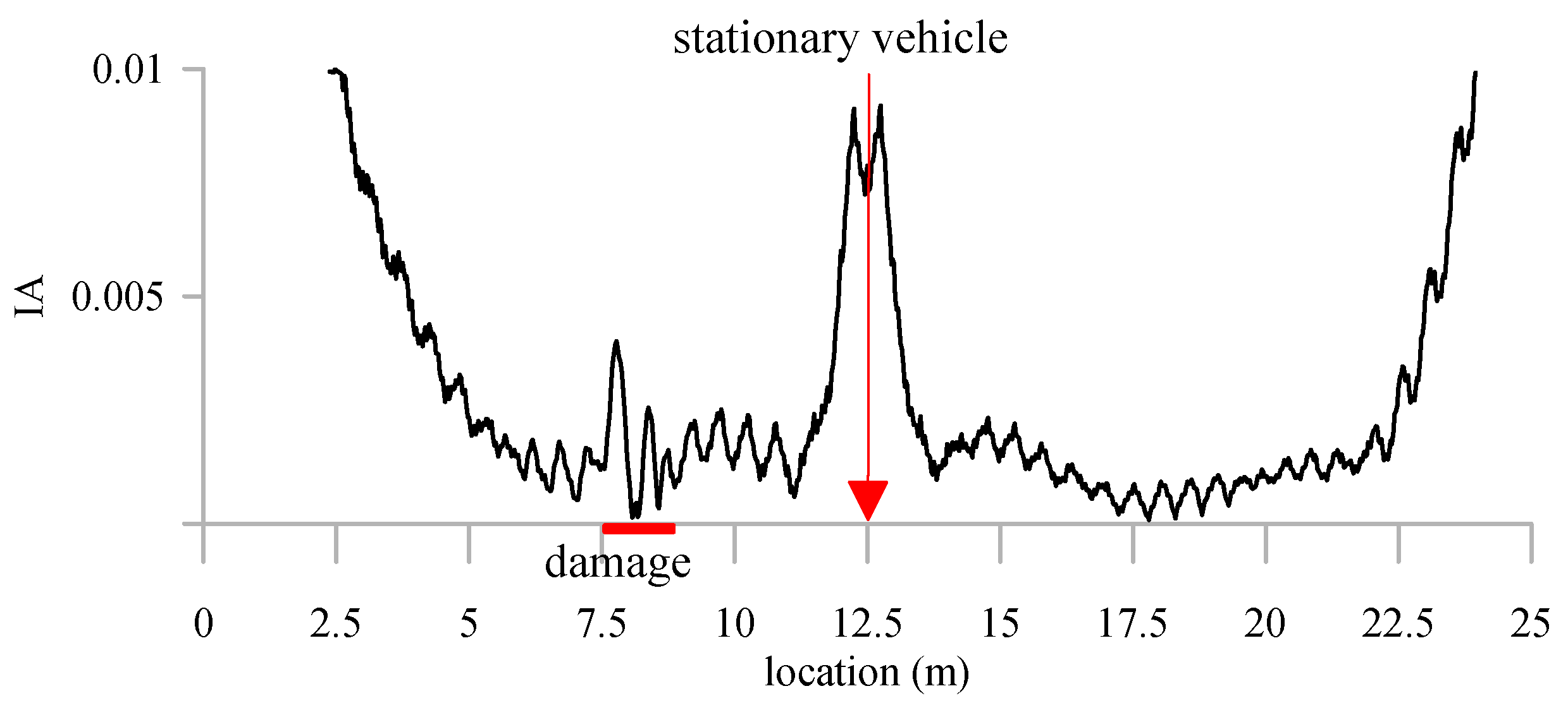
• Considering damage of 1 m in length (from 7.5 to 8.5 m away from the bridge beginning), zero damping of stationary vehicle located at mid-span, and speed of a moving vehicle of 12.5 m/s, the proposed method was able to detect the location of the damage accurately. When the location of the stationary vehicle was moved further away from the damage (20 m away from the bridge beginning), the IA also could show the peak at the correct location of the damage. After identifying the damage location from two positions of the stationary vehicle, the vehicle was stationed at the damage to investigate the response of the vehicle. In this case, only one peak of the IA appeared, and its amplitude was higher than that of the previous cases.
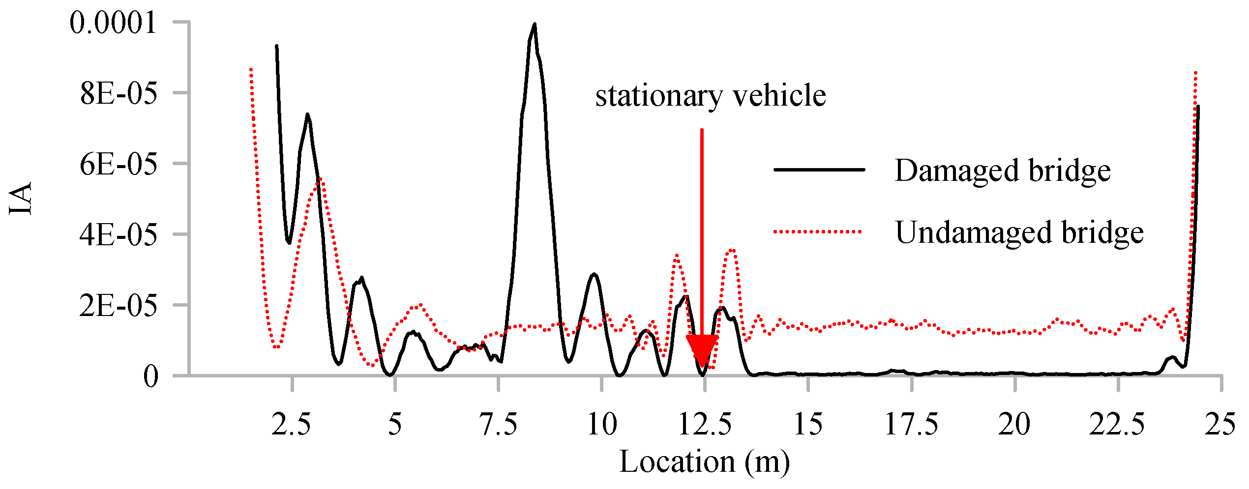
• When the IA of healthy and damaged bridge were compared, the irregularities at the bridge boundary remained similar; however, the peak that represents damage in the damaged bridge did not appear in the healthy bridge IA result. Irregularities at the boundaries do not represent damage and they occur due to the boundary condition of the bridge. Therefore, the method cannot detect damage near the boundaries of the bridge.
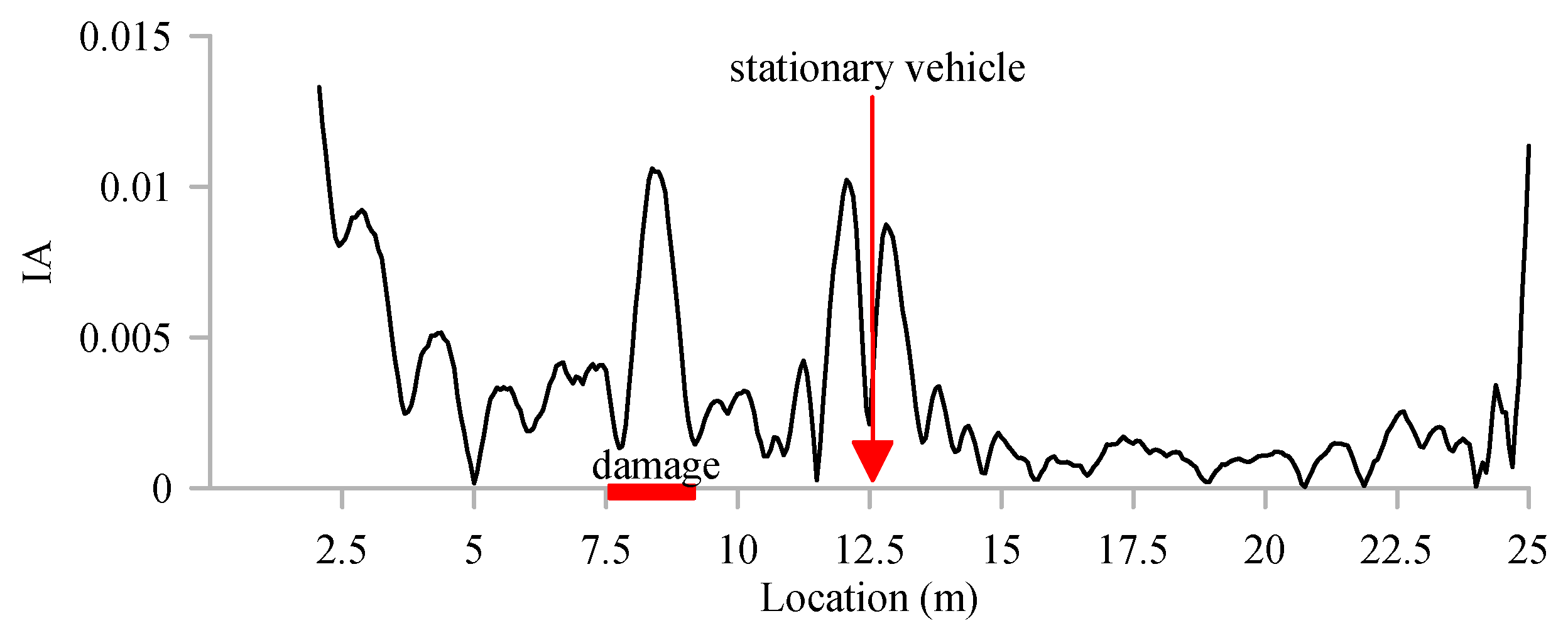
• When multiple damage was considered by adding another damage of 1 m (from 18.5 to 19.5 m) to the bridge, the proposed method could also detect the damage. Therefore, by considering the added mass of the stationary vehicle as a damage, the method could detect up to three points of damage on the bridge.
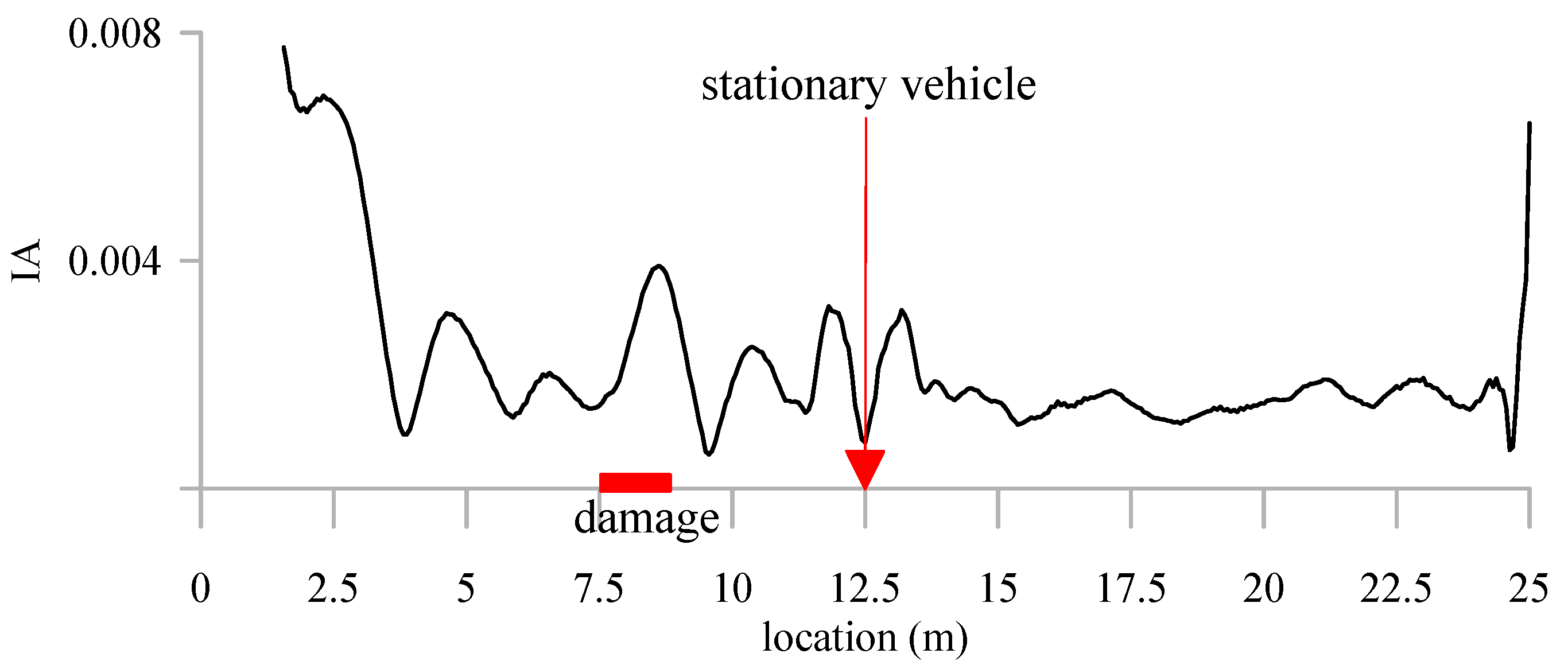
• When damping of 0.05 was added to the stationary vehicle, the vehicle was still able to detect the damage, but with less visibility. In addition, when the length of the single damage case was reduced to 0.5 m (from 8 to 8.5 m), the method could still detect the smaller damage, but with a lower visibility. Finally, when the speed of the moving vehicle was reduced to 5 m/s, lower visibility in the peak of IA was noticed.

References

1. Kim, C.W.; Chang, K.C.; McGetrick, P.J.; Inoue, S.; Hasegawa, S. Utilizing moving vehicles as sensors for bridge condition screening—A laboratory verification. Sens. Mater. 2017, 29, 153–163. [Google Scholar]
2. Hajializadeh, D. Deep-Learning-Based Drive-by Damage Detection System for Railway Bridges. Infrastructures 2022, 7, 84. [Google Scholar] [CrossRef]
3. Taha, M.M.R.; Noureldin, A.; Lucero, J.L.; Baca, T.J. Wavelet Transform for Structural Health Monitoring: A Compendium of Uses and Features. Struct. Health Monit. 2006, 5, 267–295. [Google Scholar] [CrossRef]
4. Tan, C.; Elhattab, A.; Uddin, N. Wavelet-Entropy Approach for Detection of Bridge Damages Using Direct and Indirect Bridge Records. J. Infrastruct. Syst. 2020, 26, 04020037. [Google Scholar] [CrossRef]
5. Yang, Y.-B.; Lin, C.; Yau, J. Extracting bridge frequencies from the dynamic response of a passing vehicle. J. Sound Vib. 2004, 272, 471–493. [Google Scholar] [CrossRef]
6. Lin, C.; Yang, Y.-B. Use of a passing vehicle to scan the fundamental bridge frequencies: An experimental verification. Eng. Struct. 2005, 27, 1865–1878. [Google Scholar] [CrossRef]
7. Malekjafarian, A.; McGetrick, P.J.; Obrien, E.J. A Review of Indirect Bridge Monitoring Using Passing Vehicles. Shock Vib. 2015, 2015, 286139. [Google Scholar] [CrossRef] [Green Version]
8. Malekjafarian, A.; Corbally, R.; Gong, W. A review of mobile sensing of bridges using moving vehicles: Progress to date, challenges and future trends. Structures 2022, 44, 1466–1489. [Google Scholar] [CrossRef]
9. Yang, Y.B.; Yang, J.P. State-of-the-Art Review on Modal Identification and Damage Detection of Bridges by Moving Test Vehicles. Int. J. Struct. Stab. Dyn. 2018, 18, 1850025. [Google Scholar] [CrossRef]
10. Kobayashi, Y.; Sugiura, K.; Yamaguchi, T.; Oshima, Y. Eigenfrequency estimation for bridges using the response of a passing vehicle with excitation system. In Proceedings of the Fourth International Conference on Bridge Maintenance, Safety and Management, Seoul, Korea, 13–17 July 2008. [Google Scholar] [CrossRef]
11. Yang, Y.; Chang, K.-C. Extraction of bridge frequencies from the dynamic response of a passing vehicle enhanced by the EMD technique. J. Sound Vib. 2009, 322, 718–739. [Google Scholar] [CrossRef]
12. González, A.; O’Brien, E.J.; Li, Y.-Y.; Cashell, K. The use of vehicle acceleration measurements to estimate road roughness. Veh. Syst. Dyn. 2008, 46, 483–499. [Google Scholar] [CrossRef]
13. Kim, C.-W.; Isemoto, R.; Toshinami, T.; Kawatani, M.; McGetrick, P.; O’Brien, E.J. Experimental investigation of drive-by bridge inspection. In Proceedings of the 5th International Conference on Structural Health Monitoring of Intelligent Infrastructure (SHMII-5), Cancun, Mexico, 11–15 December 2011; Instituto de Ingeniería, UNAM: Mexico City, Mexico, 2011. [Google Scholar]
14. Siringoringo, D.M.; Fujino, Y. Estimating bridge fundamental frequency from vibration response of instrumented passing vehicle: Analytical and experimental study. Adv. Struct. Eng. 2012, 15, 417–433. [Google Scholar] [CrossRef]
15. Yang, Y.; Li, Y.; Chang, K. Effect of road surface roughness on the response of a moving vehicle for identification of bridge frequencies. Interact. Multiscale Mech. 2012, 5, 347–368. [Google Scholar] [CrossRef] [Green Version]
16. Zhang, C.; Mousavi, A.A.; Masri, S.F.; Gholipour, G.; Yan, K.; Li, X. Vibration feature extraction using signal processing techniques for structural health monitoring: A review. Mech. Syst. Signal Process. 2022, 177, 109175. [Google Scholar] [CrossRef]
17. Yang, Y.B.; Li, Y.C.; Chang, K.C. Using two connected vehicles to measure the frequencies of bridges with rough surface: A theoretical study. Acta Mech. 2012, 223, 1851–1861. [Google Scholar] [CrossRef]
18. Malekjafarian, A.; O’Brien, E.J. Application of output-only modal method in monitoring of bridges using an instrumented vehicle. In Proceedings of the Civil Engineering Research in Ireland, Belfast, UK, 28–29 August 2014. [Google Scholar]
19. Yang, Y.B.; Zhang, B.; Qian, Y.; Wu, Y. Contact-Point Response for Modal Identification of Bridges by a Moving Test Vehicle. Int. J. Struct. Stab. Dyn. 2018, 18, 1850073. [Google Scholar] [CrossRef]
20. Yang, Y.; Xu, H.; Zhang, B.; Xiong, F.; Wang, Z. Measuring bridge frequencies by a test vehicle in non-moving and moving states. Eng. Struct. 2020, 203, 109859. [Google Scholar] [CrossRef]
21. Hashlamon, I.; Nikbakht, E.; Topa, A.; Elhattab, A. Numerical Parametric Study on the Effectiveness of the Contact-Point Response of a Stationary Vehicle for Bridge Health Monitoring. Appl. Sci. 2021, 11, 7028. [Google Scholar] [CrossRef]
22. Hashlamon, I.; Nikbakht, E.; Topa, A. Indirect Bridge Health Monitoring Employing Contact-Point Response of Instrumented Stationary Vehicle. In Proceedings of the International Conference on Civil, Offshore and Environmental Engineering, Dubai, United Arab Emirates, 20–21 December 2021; Springer: Berlin/Heidelberg, Germany, 2021. [Google Scholar] [CrossRef]
23. Carden, E.P.; Fanning, P. Vibration Based Condition Monitoring: A Review. Struct. Health Monit. 2004, 3, 355–377. [Google Scholar] [CrossRef]
24. Corbally, R.; Malekjafarian, A. Examining changes in bridge frequency due to damage using the contact-point response of a passing vehicle. J. Struct. Integr. Maint. 2021, 6, 148–158. [Google Scholar] [CrossRef]
25. Singh, P.; Sadhu, A. A hybrid time-frequency method for robust drive-by modal identification of bridges. Eng. Struct. 2022, 266, 114624. [Google Scholar] [CrossRef]
26. ElHattab, A.; Uddin, N.; Obrien, E. Drive-by bridge damage detection using non-specialized instrumented vehicle. Bridg. Struct. 2017, 12, 73–84. [Google Scholar] [CrossRef]
27. Janeliukstis, R.; Ručevskis, S.; Wesolowski, M.; Chate, A. Multiple Damage Identification in Beam Structure Based on Wavelet Transform. Procedia Eng. 2017, 172, 426–432. [Google Scholar] [CrossRef]
28. Bandara, S.; Rajeev, P.; Gad, E.; Sriskantharajah, B.; Flatley, I. Damage detection of in service timber poles using Hilbert-Huang transform. NDT E Int. 2019, 107, 102141. [Google Scholar] [CrossRef]
29. Kim, C.; Isemoto, R.; McGetrick, P.; Kawatani, M.; Obrien, E. Drive-by bridge inspection from three different approaches. Smart Struct. Syst. 2014, 13, 775–796. [Google Scholar] [CrossRef] [Green Version]
30. Zhu, X.; Cao, M.; Ostachowicz, W.; Xu, W. Damage Identification in Bridges by Processing Dynamic Responses to Moving Loads: Features and Evaluation. Sensors 2019, 19, 463. [Google Scholar] [CrossRef] [Green Version]
31. Mousavi, M.; Holloway, D.; Olivier, J.; Gandomi, A.H. Beam damage detection using synchronisation of peaks in instantaneous frequency and amplitude of vibration data. Measurement 2021, 168, 108297. [Google Scholar] [CrossRef]
32. McGetrick, P.J.; Kim, C.W. A Parametric Study of a Drive by Bridge Inspection System Based on the Morlet Wavelet. Key Eng. Mater. 2013, 569–570, 262–269. [Google Scholar] [CrossRef] [Green Version]
33. Hester, D.; Gonzalez, A. A discussion on the merits and limitations of using drive-by monitoring to detect localised damage in a bridge. Mech. Syst. Signal Process. 2017, 90, 234–253. [Google Scholar] [CrossRef]
34. Fitzgerald, P.; Malekjafarian, A.; Cantero, D.; Obrien, E.J.; Prendergast, L.J. Drive-by scour monitoring of railway bridges using a wavelet-based approach. Eng. Struct. 2019, 191, 1–11. [Google Scholar] [CrossRef]
35. Obrien, E.J.; Malekjafarian, A.; González, A. Application of empirical mode decomposition to drive-by bridge damage detection. Eur. J. Mech.—A/Solids 2017, 61, 151–163. [Google Scholar] [CrossRef] [Green Version]
36. Kildashti, K.; Alamdari, M.M.; Kim, C.W.; Gao, W.; Samali, B. Drive-by-bridge inspection for damage identification in a cable-stayed bridge: Numerical investigations. Eng. Struct. 2020, 223, 110891. [Google Scholar] [CrossRef]
37. Zhang, B.; Qian, Y.; Wu, Y.; Yang, Y. An effective means for damage detection of bridges using the contact-point response of a moving test vehicle. J. Sound Vib. 2018, 419, 158–172. [Google Scholar] [CrossRef]
38. Yang, Y.-B.; Zhang, B.; Qian, Y.; Wu, Y. Further Revelation on Damage Detection by IAS Computed from the Contact-Point Response of a Moving Vehicle. Int. J. Struct. Stab. Dyn. 2018, 18, 1850137. [Google Scholar] [CrossRef]
39. Zhan, Y.; Au, F.T.K.; Zhang, J. Bridge identification and damage detection using contact point response difference of moving vehicle. Struct. Control Health Monit. 2021, 28, e2837. [Google Scholar] [CrossRef]
40. Huang, N.E.; Shen, Z.; Long, S.R.; Wu, M.C.; Shih, H.H.; Zheng, Q.; Yen, N.-C.; Tung, C.C.; Liu, H.H. The empirical mode decomposition and the Hilbert spectrum for nonlinear and non-stationary time series analysis. Proc. R. Soc. Lond. Ser. A Math. Phys. Eng. Sci. 1998, 454, 903–995. [Google Scholar] [CrossRef]
41. Roveri, N.; Carcaterra, A. Damage detection in structures under traveling loads by Hilbert–Huang transform. Mech. Syst. Signal Process. 2012, 28, 128–144. [Google Scholar] [CrossRef]
42. Cheraghi, N.; Taheri, F. A damage index for structural health monitoring based on the empirical mode decomposition. J. Mech. Mater. Struct. 2007, 2, 43–61. [Google Scholar] [CrossRef]
43. Meredith, J.; González, A.; Hester, D. Empirical mode decomposition of the acceleration response of a prismatic beam subject to a moving load to identify multiple damage locations. Shock Vib. 2012, 19, 845–856. [Google Scholar] [CrossRef]
44. Dragomiretskiy, K.; Zosso, D. Variational mode decomposition. IEEE Trans. Signal Process. 2013, 62, 531–544. [Google Scholar] [CrossRef]
45. ISO 8608; Mechanical Vibration–Road Surface Profiles–Reporting of Measured Data. ISO: London, UK, 2016.
46. He, W.-Y.; Ren, W.-X. Structural damage detection using a parked vehicle induced frequency variation. Eng. Struct. 2018, 170, 34–41. [Google Scholar] [CrossRef]
Figure 1. Schematic representation the proposed damage detection method.
Applsci 12 11625 g001
Figure 2. A stationary vehicle parked in the middle of a bridge while another moving vehicle passes over the bridge.
Applsci 12 11625 g002
Figure 3. A typical profile of road surface roughness.
Applsci 12 11625 g003
Figure 4. Dynamic response of the stationary vehicle, its contact-point, and bridge acceleration response at mid-span.
Applsci 12 11625 g004
Figure 5. IA of the contact-point response of a stationary vehicle parked at mid-span.
Applsci 12 11625 g005
Figure 6. IA of the contact-point response of a stationary vehicle parked far from the location of the damage.
Applsci 12 11625 g006
Figure 7. IA of the contact-point response of a stationary vehicle parked at the location of the damage.
Applsci 12 11625 g007
Figure 8. IA of the IMF for the healthy and damaged bridge.
Applsci 12 11625 g008
Figure 9. IA of the IMF of contact-point response of the damped stationary vehicle.
Applsci 12 11625 g009
Figure 10. IA of the IMF of contact-point response of the stationary vehicle on a bridge with multiple damage.
Applsci 12 11625 g010
Figure 11. IA of IMF of contact-point response of a stationary vehicle on a bridge with 0.5 m damage size.
Applsci 12 11625 g011
Figure 12. IA of IMF of the contact-point response of a stationary vehicle with 5 m/s speed of the moving vehicle.
Applsci 12 11625 g012