Flood Prediction with Two-Dimensional Shallow Water Equations: A Case Study of Tongo-Bassa Watershed in Cameroon

Abstract

As a result of urbanization, combined with the anthropogenic effects of climate change, natural events such as floods are showing increasingly adverse impacts on human existence. This study proposes a new model, based on shallow water equations, that is able to predict these floods and minimize their impacts. The first-order finite volume method (FVM), the Harten Lax and van Leer (HLL) scheme, and the monotone upwind scheme for conservation laws (MUSCL) are applied in the model. In addition, a virtual boundary cell approach is adopted to achieve a monotonic solution for both interior and boundary cells and flux computations at the boundary cells. The model integrates the infiltration parameters recorded in the area, as well as the Manning coefficient specific to each land-cover type of the catchment region. The results provided were mapped to highlight the potential flood zones and the distribution of water heights throughout the catchment region at any given time, as well as that at the outlet. It has been observed that when standard infiltration and the Manning parameters were selected, the floodable surface increased, as expected, with the increasing rainfall intensity and duration of the simulation. With sufficient infiltration, only a portion of the water tends to stagnate and flow off on the surface toward the outlet. A sensitivity analysis of certain parameters, such as rainfall data and the final infiltration coefficient in the lower watershed of the littoral region, was conducted; the results show that the model simulates well the general character of water flow in the watershed. Finally, the model’s validation using field-collected parameters during the flood of 25 July 2017 and 18 to 22 July 2016 in the Grand Ouaga basin in Burkina reveals Nash–Sutcliffe values of 0.7 and 0.73, respectively.

1. Introduction

The global increase in urban populations has led to a corresponding increase in the demand for infrastructure, including buildings, roads, and drainage networks [1]. The implementation of these infrastructures has led to a reduction in rainwater absorption capacities, exposing urban vulnerabilities during flooding in the presence of heavy rain events [2,3]. Furthermore, the climatic changes that have become accentuated over the last few decades have tended to cause an increase in the frequency, intensity, and duration of rain events in many countries [1,4]. Natural disasters resulting from high-water events, such as glacial melting, droughts, storms, and floods are being exacerbated by frequent extreme weather occurrences that are driven by climate change [5,6]. These “high-water events” could be described as “water overflowing its natural or manmade banks into ordinarily dry terrain, such as a river inundating its floodplain” [7].

Flooding is perhaps the most catastrophic natural disaster, wreaking havoc on human lives and the economy while damaging infrastructure (bridges, buildings, etc.) [8]. For example, significant damage was recorded in Australia in the Brisbane region at the beginning of 2011, as a result of flooding [9].

Furthermore, massive floods in the Mississippi River basin in the United States have been caused by rainfall, coupled with spring snowmelt, resulting in damage estimated to cost billions of dollars. The 2007 floods in the United Kingdom (UK) caused 42,000 individuals to lose electricity for more than 24 h, while 350,000 others lost their water supply for up to 17 days, and over 10,000 of the latter group became stranded on roads and trains [10]. The most expensive flood damage in history occurred in Thailand’s Chao Praya River Basin, as a result of persistent floods. The cost of the damage was estimated to be over USD 45 billion [11,12] reported that in the USA alone, flood management infrastructure interventions have helped to save 10 million acres of land and almost one million acres from flooding, averting more than USD 110 billion in flood damage costs. The lack of flood management infrastructure has long been a concern for researchers. More recently, the Ministry of Humanitarian Affairs, Disaster Management, and Social Development of Nigeria published a report of the damage caused by the floods earlier in October 2022. The balance sheet shows that more than 1.4 million people have been affected by the floods; an estimated 500 people were killed, with 1546 others injured and 790,254 persons displaced. One month later, the National Emergency Management Agency (NEMA) of Nigeria said that at least 300 people had died and more than 100,000 others had been displaced since the start of the rainy season and with the release of excess water from a dam in neighboring Cameroon. This assessment was recorded as the most catastrophic event compared to the last major floods of 2012 (https://edition.cnn.com/2022/10/13/africa/hundreds-killed-nigeria-floods-intl, accessed on 13 October 2022). Ref. [13] studied the history of flash-flood occurrence in a southern Italy drainage basin, to identify the real cause of the increment in flood occurrence. The study compared rainfall to anthropogenic modifications and concluded that the rainfall in the study area had a decreasing trend while flood damage still increased, showing that the real cause of flash floods in the area was mismanagement and land-use modification. Floods have become more common in various nations around the world in recent decades, prompting governments and experts to collaborate on flood management and prevention techniques [14,15].

It is, therefore, important to pay attention to the behavior of water and flood systems. Numerical and experimental approaches have been applied to investigate the flooding issue and water behavior [16] using the shallow water equations developed by Saint-Venant in 1871 [17]. These equations constitute the fundamental basis for the development of numerical models for open channel flow. Two types of numerical models were developed to investigate flood-wave propagation in one dimension [18,19,20,21,22] and two dimensions [23,24,25]. Following the Nari typhoon in Taiwan, ref. [26] reproduced the flood occurrence by comparing the numerical model output with the pumped water volume obtained from the subway system, along with the failure time of several pump stations. They compared the results of their numerical model to the data gathered in the field. The massive flooding event in Sumacarcel, Spain, was caused by the breakdown of the Tous Dam in October 1982 and was also investigated numerically by [27]. They collected water-depth elevation data by conducting interviews and reviewing the Centre for Studies and Experimentation of the Ministry of Public Works (CEDEX, Spain) reports. Ref. [28] simulated the Nîmes flood event and the numerical results were compared to the historical data. Ref. [29] represented the roughness effects of structures in flood-prone urban areas, eventually formulating a numerical simulation model. The creation of dedicated computer tools has heavily contributed to the development and implementation of software capable of efficiently simulating floods. Using the Medjerda River in Tunisia as an example, a comparison of 1Dimension and 2Dimension hydraulic models for floods has been performed by [30].

The Hydrological Engineering Center’s river analysis system (HEC RAS) and MIKE 11 are used in the one-dimensional models, whereas TELEMAC 2D is used in two-dimensional models. In addition, [31] developed an operational forecasting system (OFS) for better flash flood prediction and warnings in mountainous regions. The developed system uses high-density and high-accuracy airborne LiDAR DEM data to simulate rapid water-level rises and flooding as the result of intense rainfall within relatively small watersheds. The results revealed that the water levels and flood extent derived from the OFS produced agreements between the measured and surveyed data. More recently, [32] developed a high-performance two-dimensional hydrodynamic model based on the finite element method and unstructured grids. They combined the weather research and forecasting (WRF) model, the storm water management model (SWMM), a two-dimensional hydrodynamic model, and a map-oriented visualization tool to operational high performance. They concluded that the extent of flooding during historical inundation events, as derived from the forecasting systems, agrees well with the surveyed data for plain areas in southwestern Taiwan. Despite the development of several numerical flood simulation models, such as the finite difference method (FDM) [33], the finite volume method (FVM) [34], and dedicated software [35], the issue of prediction and prevention is still relevant. Some of these previous models failed to address the issue of flow simulation, not only due to the difficulty in access (due to the high cost) and handling for the majority of the population but also due to the rigidity of certain parameters used in the software, which prevented them from being adjusted to the case study and for sensitivity to the basin’s topography. Another drawback was their inability to forecast and emphasize those regions that would flood and how the water levels in the study area were distributed. In order to considerably reduce the damage and disasters linked to the sudden occurrence of floods, therefore, it appears necessary to develop a model capable of predicting the flood zones as well as the water depths for a given watershed. This would not only identify those areas at risk where populations should be prohibited from settling but also provide estimates of the time required for a rapid evacuation operation in the event of an emergency.

The new flood simulation method which is a combination of previous numerical models and field-estimated parameters, developed in this paper gives a more detailed representation of the surface flow and makes a reasonable approximation of the hydrology. Moreover, the model can predict the distribution of water height in a catchment area, as well as the height and flow discharge at the outlet. To build the model, the finite volume method (FVM)–Godunov type is adopted to solve the 2D shallow-water equation, and the monotonic upstream-centered scheme for conservation laws (MUSCL)–Hancock scheme has been associated with the model to provide high-accuracy numerical solutions to the partial differential equations, which can involve solutions that exhibit shocks or discontinuities. The main goal of using the MUSCL scheme in the model is to replace the piecewise constant approximation of Godunov’s scheme with reconstructed states, derived from cell-averaged states obtained from the previous time step. The structured grid was chosen for its ease of implementation, and the fluxes were computed using the Harten Lax and van Leer (HLL) approximation Riemann solution. The model is sensitive to the topography of the free surface of water flow, which results in the integration of roughness or the Manning coefficient. A virtual boundary cell is also used to compute the flux in different cells by coupling the Riemann invariant with a head-flow boundary at time M and N respectively in the x and y direction [36]. Furthermore, the model also considers the daily rainfall or rainfall data recorded in a given space, along with the infiltration parameters specific to each type of soil. Estimates of surface evaporation of the basin and the flow rate will then be integrated into the numerical equations to add further realism. The Courant number used in the stability of unstable numerical methods and the simulation time have also been incorporated into the model.

To demonstrate the model’s power, this work models the response of the Tongo-Bassa catchment in Douala-Cameroon by using a new model integrating the parameters from the field and validating the model by means of another catchment called Grand-Ouaga in Burkina Faso.

The following sections briefly discuss the 2D governing equation of the surface flow problem, before providing general information on the research area, the numerical strategy for solving it, and an examination of how well the different numerical approaches perform in the field.

2. Numerical Model

2.1. Mathematical Equations

The conservative form of the 2D shallow water equations, derived from the Navier–Stocks equations by considering the viscous, source, and friction terms are presented as follows:

$$\frac{\partial \mathrm{U}}{\partial \mathrm{t}}+\frac{\partial \mathrm{F}\left(\mathrm{U}\right)}{\partial \mathrm{x}}+\frac{\partial \mathrm{G}\left(\mathrm{U}\right)}{\partial \mathrm{y}}={\mathrm{S}}_{\mathrm{s}}+{\mathrm{S}}_{\mathrm{f}}+{\mathrm{S}}_{\mathrm{p}}$$

(1)

where x and y represent the Cartesian coordinates; t is the time; U is the conservative variables; F and G are the flux vectors in the x and y directions, respectively. The bottom slope, the friction terms, and the source term are expressed by ${\mathrm{S}}_{\mathrm{s}}$, ${\mathrm{S}}_{\mathrm{f}}$, and ${\mathrm{S}}_{\mathrm{p}}$, respectively. The bottom slope, friction terms, source term, and flux vectors are defined as:

• The flux vectors F and G:

$$\mathrm{F}\left(\mathrm{U}\right)=\left[\begin{array}{c}\mathrm{hu}\\ {\mathrm{hu}}^2+\frac{1}{2}{\mathrm{gh}}^2\\ \mathrm{huv}\end{array}\right]; \mathrm{G}\left(\mathrm{U}\right)=\left[\begin{array}{c}\mathrm{hv}\\ \mathrm{huv}\\ {\mathrm{hv}}^2+\frac{1}{2}{\mathrm{gh}}^2\end{array}\right]$$

(2)

where h is the water height; g is the gravitational acceleration; u and v are the depth-averaged velocity components in the x and y directions.

• The bottom slope$S_s$, friction$S_{f,}$and source$S_p$:

$${\mathrm{S}}_{\mathrm{s}}=\left[\begin{array}{c}0\\ -\mathrm{gh}\frac{\partial \mathrm{z}}{\partial \mathrm{x}}\\ -\mathrm{gh}\frac{\partial \mathrm{z}}{\partial \mathrm{y}}\end{array}\right];{ \mathrm{S}}_{\mathrm{f}}=\left[\begin{array}{c}0\\ -{\mathrm{nm}}^2\frac{\sqrt{{\mathrm{u}}^2+{\mathrm{v}}^2}}{{\mathrm{h}}^{\frac{4}{3}}}\mathrm{u}\\ -{\mathrm{nm}}^2\frac{\sqrt{{\mathrm{u}}^2+{\mathrm{v}}^2}}{{\mathrm{h}}^{\frac{4}{3}}}\mathrm{v}\end{array}\right];{ \mathrm{S}}_{\mathrm{p}}=\left[\begin{array}{c}\mathrm{P}-\left(\mathrm{I}-\mathrm{E}-\mathrm{q}\right)\\ 0\\ 0\end{array}\right]$$

(3)

where $-\frac{\partial \mathrm{z}}{\partial \mathrm{x}}$ and $-\frac{\partial \mathrm{z}}{\partial \mathrm{y}}$ are the bed slopes in the x and y directions, respectively; z is the bed elevation; nm is the Manning–Strickler coefficient; P and I are the rainfall intensity (mm/min) and infiltration rate; E is the surface evaporation (mm/min) and q is the flow rate. Horton’s infiltration model, developed in the 1930s, has been used to calculate the infiltration rate [37]. The model indicates that infiltration tends to decrease exponentially if the rainfall exceeds the infiltration capacity. The formula is expressed as:

$$\mathrm{I}\left(t_s\right)={\mathrm{i}}_{\mathrm{f}}+\left({\mathrm{i}}_0-{\mathrm{i}}_{\mathrm{f}}\right)\exp \left(-\mathrm{r}{t}_s\right)$$

(4)

where ${\mathrm{i}}_0$, ${\mathrm{i}}_{\mathrm{f}}$, r, and $t_s$ are, respectively, the initial infiltration rate (mm/min), the final infiltration rate (mm/min), a constant depending on soil properties (min⁻¹), and the duration of the storm (min).

2.1.1. Discretization of the Shallow-Water Equation

The FVM-Godunov approach solves the two-dimensional shallow-water equations by integrating the source term.

$${\mathrm{U}}_{\mathrm{t}}+\mathrm{F}{\left(\mathrm{U}\right)}_{\mathrm{x}}+\mathrm{G}{\left(\mathrm{U}\right)}_{\mathrm{y}}=\mathrm{S}\left(\mathrm{U}\right)$$

(5)

By integrating Equation (6) into each cell and time step, the formulation becomes:

$${{\displaystyle \int }}_{{\mathrm{x}}_{\mathrm{i}-1/2}}^{{\mathrm{x}}_{\mathrm{i}+1/2}}{{\displaystyle \int }}_{{\mathrm{y}}_{\mathrm{j}-1/2}}^{{\mathrm{y}}_{\mathrm{j}+1/2}}{{\displaystyle \int }}_{{\mathrm{t}}^{\mathrm{n}}}^{{\mathrm{t}}^{\mathrm{n}+1}}\left(\frac{\partial \mathrm{U}}{\partial \mathrm{t}}+\frac{\partial \left(\mathrm{F}\left(\mathrm{U}\right)\right)}{\partial \mathrm{x}}+\frac{\partial \left(\mathrm{G}\left(\mathrm{U}\right)\right)}{\partial \mathrm{y}}\right)\mathrm{dxdydt}={{\displaystyle \int }}_{{\mathrm{x}}_{\mathrm{i}-1/2}}^{{\mathrm{x}}_{\mathrm{i}+1/2}}{{\displaystyle \int }}_{{\mathrm{y}}_{\mathrm{j}-1/2}}^{{\mathrm{y}}_{\mathrm{j}+1/2}}{{\displaystyle \int }}_{{\mathrm{t}}^{\mathrm{n}}}^{{\mathrm{t}}^{\mathrm{n}+1}}\left(\mathrm{S}\left(\mathrm{U}\right)\right)\mathrm{dxdydt} .$$

(6)

For a better resolution of Equation (7) and to ensure its stability, system decomposition is recommended. This will have to be performed in the x-direction on the one hand and the y-direction on the other hand.

The resolution is split into a sequence of one-dimensional equations.

In the x-direction:

$${{\displaystyle \int }}_{{\mathrm{x}}_{\mathrm{i}-1/2}}^{{\mathrm{x}}_{\mathrm{i}+1/2}}{{\displaystyle \int }}_{{\mathrm{t}}^{\mathrm{n}}}^{{\mathrm{t}}^{\mathrm{n}+1}}\left(\frac{\partial \mathrm{U}}{\partial \mathrm{t}}+\frac{\partial \left(\mathrm{F}\left(\mathrm{U}\right)\right)}{\partial \mathrm{x}}\right)\mathrm{dxdt}=0 .$$

(7)

The numerical solution at time $t_{n+1/4}$ is obtained from the resolution of Equation (8), as follows:

$$\frac{U_{i,j}^{n+1/4}-U_{i,j}^n}{\Delta t}+\frac{F_{i+1/2,j}^n-F_{i-1/2,j}^n}{\Delta x}=0$$

(8)

where $U_{i,j}^n$ is the first solution along each row of cells, with j fixed; $F_{i+1/2,j}^n$ is the numerical flux between two consecutive cells (i−1, j) and (i, j).

Then, we solve the equation again, this time along the y-direction.

$${{\displaystyle \int }}_{{\mathrm{y}}_{\mathrm{i}-1/2}}^{{\mathrm{y}}_{\mathrm{i}+1/2}}{{\displaystyle \int }}_{{\mathrm{t}}^{\mathrm{n}}}^{{\mathrm{t}}^{\mathrm{n}+1}}\left(\frac{\partial \mathrm{U}}{\partial \mathrm{t}}+\frac{\partial \left(\mathrm{G}\left(\mathrm{U}\right)\right)}{\partial \mathrm{y}}\right)\mathrm{dydt}=0$$

(9)

The numerical solution at time $t_{n+2/4}$ is obtained from the resolution of Equation (10), as follows:

$$\frac{U_{i,j}^{n+2/4}-U_{i,j}^{n+1/4}}{\Delta t}+\frac{G_{i+1/2,j}^{n+1/4}-G_{i-1/2,j}^{n+1/4}}{\Delta y}=0$$

(10)

where $U_{i,j}^{n+1/4}$ are present as data along each row of cells, with i fixed; $G_{i-1/2,j}^{n+1/4}$ is the numerical flux between two consecutive cells (i,j−1) and (i,j).

The integration of the friction and source terms (rainfall, infiltration, and bottom slope) are established as follows:

$$\frac{U_{i,j}^{n+\frac{3}{4}}-U_{i,j}^{n+\frac{2}{4}}}{\Delta t}=S_f\left(U_{i,j}^{n+\frac{2}{4}}\right)+S_S\left(U_{i,j}^{n+\frac{2}{4}}\right);$$

(11)

$$\frac{U_{i,j}^{n+1}-U_{i,j}^{n+\frac{3}{4}}}{\Delta t}=S_p\left(U_{i,j}^{n+\frac{3}{4}}\right) .$$

(12)

2.1.2. Integration of the Topography

The method of solving the equations by decomposition, which considers the system as homogeneous, as seen above, could not be used in the context of topography because such an approach yields poor results when U corresponds to a stationary state. It can be expressed as:

$$\{\begin{array}{c}u=0\\ \frac{\partial \left(\frac{1}{2}{\mathrm{gh}}^2\right)}{\partial \mathrm{x}}=-\mathrm{gh}\frac{\partial \mathrm{Z}}{\partial \mathrm{x}}\end{array} .$$

(13)

The following Equation (11) can be resumed as a constant, namely:

$$\mathrm{H}=\mathrm{h}+\mathrm{Z}$$

(14)

where H is the water level.

H is a constant; this state physically corresponds to the state of equilibrium of the watercourse or steady state. The hydrostatic reconstruction proposed by [38], coupled with a positive numerical flux, allows us to verify important mathematical and physical properties, such as the positivity of the water height, and, thus, to avoid instabilities when dealing with dry zones. The equations are as follows:

$$\{\begin{array}{c}{\mathrm{h}}_{\mathrm{i}+\frac{1}{2}\mathrm{L}}=\max \left({\mathrm{h}}_{\mathrm{i}}+{\mathrm{Z}}_{\mathrm{i}}-\max \left({\mathrm{Z}}_{\mathrm{i}},{\mathrm{Z}}_{\mathrm{i}+1}\right),0\right)\\ \begin{array}{c}{\mathrm{h}}_{\mathrm{i}+\frac{1}{2}\mathrm{R}}=\max \left({\mathrm{h}}_{\mathrm{i}+1}+{\mathrm{Z}}_{\mathrm{i}+1}-\max \left({\mathrm{Z}}_{\mathrm{i}},{\mathrm{Z}}_{\mathrm{i}+1}\right),0\right)\\ {\mathrm{U}}_{\mathrm{i}+\frac{1}{2}\mathrm{L}}=\left({\mathrm{h}}_{\mathrm{i}+\frac{1}{2}\mathrm{L}},{\mathrm{h}}_{\mathrm{i}+\frac{1}{2}\mathrm{L}}{*\mathrm{u}}_{\mathrm{i}}\right)\end{array}\\ {\mathrm{U}}_{\mathrm{i}+\frac{1}{2}\mathrm{R}}=\left({\mathrm{h}}_{\mathrm{i}-\frac{1}{2}\mathrm{R}},{\mathrm{h}}_{\mathrm{i}-\frac{1}{2}\mathrm{R}}{*\mathrm{u}}_{\mathrm{i}}\right)\end{array}$$

(15)

The water height computed on the left and right sides of the cell, respectively, are expressed as ${\mathrm{h}}_{\mathrm{i}+\frac{1}{2}\mathrm{L}}$ and ${\mathrm{h}}_{\mathrm{i}+\frac{1}{2}\mathrm{R}}$; the general solutions found at the left and right sides of each cell are represented respectively as ${\mathrm{U}}_{\mathrm{i}+\frac{1}{2}\mathrm{L}}$ and ${\mathrm{U}}_{\mathrm{i}+\frac{1}{2}\mathrm{R}}$. The numerical schema can now be written as:

$${\mathrm{U}}_{\mathrm{i}}^{\mathrm{n}+1}-{\mathrm{U}}_{\mathrm{i}}^{\mathrm{n}}+\frac{\Delta \mathrm{t}}{\Delta \mathrm{x}}\left({\mathrm{F}}_{\mathrm{i}+\frac{1}{2}\mathrm{L}}^{\mathrm{n}}-{\mathrm{F}}_{\mathrm{i}-\frac{1}{2}\mathrm{R}}^{\mathrm{n}}\right)=0$$

(16)

where:

$${\mathrm{F}}_{\mathrm{i}-\frac{1}{2}\mathrm{R}}^{\mathrm{n}}={\mathrm{F}}_{\mathrm{i}-\frac{1}{2}}^{\mathrm{n}}+{\mathrm{S}}_{\mathrm{i}-\frac{1}{2}\mathrm{R}}{ \mathrm{and} \mathrm{F}}_{\mathrm{i}+\frac{1}{2}\mathrm{L}}^{\mathrm{n}}={\mathrm{F}}_{\mathrm{i}+\frac{1}{2}}^{\mathrm{n}}+{\mathrm{S}}_{\mathrm{i}+\frac{1}{2}\mathrm{L}}$$

(17)

$${\mathrm{S}}_{\mathrm{i}-\frac{1}{2}\mathrm{R}}=\left(\begin{array}{c}0\\ \mathrm{P}\left({\mathrm{h}}_{\mathrm{i}}^{\mathrm{n}}\right)-\mathrm{P}\left({\mathrm{h}}_{\mathrm{i}+\frac{1}{2}\mathrm{L}}^{\mathrm{n}}\right)\end{array}\right){ \mathrm{and} \mathrm{S}}_{\mathrm{i}+\frac{1}{2}\mathrm{L}}=\left(\begin{array}{c}0\\ \mathrm{P}\left({\mathrm{h}}_{\mathrm{i}}^{\mathrm{n}}\right)-\mathrm{P}\left({\mathrm{h}}_{\mathrm{i}+\frac{1}{2}\mathrm{L}}^{\mathrm{n}}\right)\end{array}\right),$$

(18)

where the hydrostatic pressure is given by $\mathrm{P}\left(\mathrm{h}\right)=\frac{1}{2}{\mathrm{gh}}^2$.

2.1.3. Integration of Rainfall Intensity

The rainfall intensity can be computed through integration, as follows:

$${{\displaystyle \int }}_{{\mathrm{x}}_{\mathrm{i}-\frac{1}{2}}}^{{\mathrm{x}}_{\mathrm{i}+\frac{1}{2}}}{{\displaystyle \int }}_{{\mathrm{t}}^{\mathrm{n}}}^{{\mathrm{t}}^{\mathrm{n}+1}}\left(\frac{\partial \mathrm{h}}{\partial \mathrm{t}}\right)\mathrm{dxdt}={{\displaystyle \int }}_{{\mathrm{x}}_{\mathrm{i}-\frac{1}{2}}}^{{\mathrm{x}}_{\mathrm{i}+\frac{1}{2}}}{{\displaystyle \int }}_{{\mathrm{t}}^{\mathrm{n}}}^{{\mathrm{t}}^{\mathrm{n}+1}}\left(\mathrm{P}\left(\mathrm{h}\right)-\mathrm{i}\left(\mathrm{t}\right)\right)\mathrm{dxdt}$$

(19)

The resolution of Equation (17) yields:

$${\mathrm{h}}_{\mathrm{i}}^{\mathrm{n}+\frac{1}{2}}={\mathrm{h}}_{\mathrm{i}}^{\mathrm{n}}+\frac{\mathrm{dt}}{2}{\mathrm{P}}_{\mathrm{i}}^{\mathrm{n}}-\left(\mathrm{I}\left({\mathrm{t}}^{\mathrm{n}+\frac{1}{2}}\right)-\mathrm{I}\left({\mathrm{t}}^{\mathrm{n}}\right)\right)$$

(20)

The Horton model appears to be the best for the management of infiltration but that model can face certain problems, due to the heterogeneity of the infiltration and rainfall parameters. Furthermore, the model’s runoff is generated not only by rain that supplies water to a cell but also by flowing from another cell. The amount of water available for infiltration on a cell at time $t^n$ is given as:

$${\mathrm{w}}_{\mathrm{i}}^{\mathrm{n}}=\frac{2}{\mathrm{dt}}{\mathrm{h}}_{\mathrm{i}}^{\mathrm{n}}+{\mathrm{P}}_{\mathrm{i}}^{\mathrm{n}}$$

(21)

A comparison should then be made between the infiltration and the water available in each cell. Now we have:

$$\{\begin{array}{c}{\mathrm{I}}_{\mathrm{i}}^{\mathrm{n}+\frac{1}{2}}={\mathrm{I}}_{\mathrm{i}}^{\mathrm{n}}+\frac{\mathrm{dt}}{2}{\mathrm{P}}_{\mathrm{i}}^{\mathrm{n}}+{\mathrm{h}}_{\mathrm{i}}^{\mathrm{n}} \mathrm{if} W\le i\left(t\right)\\ {\mathrm{I}}_{\mathrm{i}}^{\mathrm{n}+\frac{1}{2}}-{\mathrm{I}}_{\mathrm{i}}^{\mathrm{n}}={\mathrm{i}}_{\mathrm{f}}{\mathrm{t}}^{\mathrm{n}}+\frac{\left({\mathrm{i}}_{\mathrm{o}}-{\mathrm{i}}_{\mathrm{f}}\right)\left(1-{\mathrm{e}}^{-{\mathrm{rt}}^{\mathrm{n}}}\right)}{\mathrm{r}} \mathrm{if} W\ge i\left(t\right)\end{array}$$

(22)

In the case where $\mathrm{W}\le \mathrm{i}\left(\mathrm{t}\right),$ then water height is assumed to be constant, namely, ${\mathrm{h}}_{\mathrm{i}}^{\mathrm{n}+\frac{1}{2}}=0$, but if $\mathrm{W}\ge \mathrm{i}\left(\mathrm{t}\right)$, the water height should be considered as:

$${\mathrm{h}}_{\mathrm{i}}^{\mathrm{n}+\frac{1}{2}}={\mathrm{h}}_{\mathrm{i}}^{\mathrm{n}}+\frac{\mathrm{dt}}{2}{\mathrm{P}}_{\mathrm{i}}^{\mathrm{n}}-\left({\mathrm{i}}_{\mathrm{f}}{\mathrm{t}}^{\mathrm{n}}+\frac{\left({\mathrm{i}}_{\mathrm{o}}-{\mathrm{i}}_{\mathrm{f}}\right)\left(1-{\mathrm{e}}^{-{\mathrm{rt}}^{\mathrm{n}}}\right)}{\mathrm{r}}\right).$$

(23)

2.1.4. Computation of the Flow Rate

The surface of the basin where the runoff is supposed to take place can be assumed to be a rectangular channel, with $l$ as the width, D-Ds as the height, and a slope of S. The flow can be computed using the Manning equation, as follows:

$$Q=\frac{1.49}{nm}{S}^{0.5}{R}_H^{2/3}{A}_S$$

(24)

where:

nm is the roughness coefficient;

$A_s$ is the surface of the basin crossed by the runoff ($A_s=l\ast \left(D-Ds\right)$;

$R_H$ is the hydraulic radius ($R_H=D-Ds)$;

A is the surface of the basin or catchment;

D is the height from the impervious area in the soil until the surface runoff;

Ds is the thickness between the soil surface and the impervious area of the soil.

At this point, the flow rate can be determined using the following equation.

If $(\mathrm{D}>\mathrm{Ds})$:

$$q=\frac{1.49}{A\ast nm}l\ast S^{0.5}\ast {\left(D-Ds\right)}^{5/3} .$$

(25)

In the case where $\left(\mathrm{D}\le \mathrm{Ds}\right),$ then $q=0$.

2.2. Numerical Flux Computation

Among the different numeric fluxes developed in the past, [39] proposed the HLL scheme (Harten–Lax–Leer) [40]) as the most stable method and the one best able to compute fluxes F and G for this case. They suggested the following HLL fluxes at the cell interfaces.

• The computation of the F flux:

$$\mathrm{F}\left({\mathrm{U}}_{\mathrm{L}},{\mathrm{U}}_{\mathrm{R}}\right)=\{\begin{array}{c}\mathrm{F}\left({\mathrm{U}}_{\mathrm{L}}\right)\hspace{1em}\hspace{1em}\hspace{1em}\hspace{1em}\hspace{1em}\hspace{1em}\hspace{1em}\hspace{1em}\hspace{1em}\mathrm{if} 0\le {\mathrm{C}}_1^{\mathrm{x}}\\ \frac{{\mathrm{C}}_2^{\mathrm{x}}\mathrm{F}\left({\mathrm{U}}_{\mathrm{L}}\right)-{\mathrm{C}}_1^{\mathrm{x}}\mathrm{F}\left({\mathrm{U}}_{\mathrm{R}}\right)+{\mathrm{C}}_1^{\mathrm{x}}{\mathrm{C}}_2^{\mathrm{x}}\left({\mathrm{U}}_{\mathrm{R}}-{\mathrm{U}}_{\mathrm{L}}\right)}{{\mathrm{C}}_2^{\mathrm{x}}-{\mathrm{C}}_1^{\mathrm{x}}}\\ \mathrm{F}\left({\mathrm{U}}_{\mathrm{R}}\right){\hspace{1em}\hspace{1em}\hspace{1em}\hspace{1em}\hspace{1em}\hspace{1em}\hspace{1em}\hspace{1em}\hspace{1em}\mathrm{if} \mathrm{C}}_2^{\mathrm{x}}\le 0\end{array}{ \mathrm{if} \mathrm{C}}_1^{\mathrm{x}}<0<{\mathrm{C}}_2^{\mathrm{x}}$$

(26)

where ${\mathrm{U}}_{\mathrm{L}}$ and ${\mathrm{U}}_{\mathrm{R}}$ are, respectively, the left and right approximations of the solution in the cell. The coefficients ${\mathrm{C}}_1^{\mathrm{x}}$ et ${\mathrm{C}}_2^{\mathrm{x}}$ are calculated as:

$${\mathrm{C}}_1^{\mathrm{x}}=\underset{\mathrm{U}={\mathrm{U}}_{\mathrm{L}},{\mathrm{U}}_{\mathrm{R}}}{\min }(\underset{\mathrm{j}=1,2,3}{\min }{\mathsf{\beta }}_{\mathrm{j}}^{\mathrm{x}}\left(\mathrm{U}\right));{ \mathrm{C}}_2^{\mathrm{x}}=\underset{\mathrm{U}={\mathrm{U}}_{\mathrm{L}},{\mathrm{U}}_{\mathrm{R}}}{\max }(\underset{\mathrm{j}=1,2,3}{\max }{\mathsf{\beta }}_{\mathrm{j}}^{\mathrm{x}}\left(\mathrm{U}\right))$$

(27)

where the term ${\mathsf{\beta }}_{\mathrm{j}}^{\mathrm{x}}$, with j = 1, 2, 3, represents the eigenvalues of the Jacobian of F and can be expressed as:

$${\mathsf{\beta }}_1^{\mathrm{x}}=\mathrm{u}-\sqrt{\mathrm{gh}},{ \mathsf{\beta }}_2^{\mathrm{x}}=\mathrm{u},{ \mathsf{\beta }}_3^{\mathrm{x}}=\mathrm{u}+\sqrt{\mathrm{gh}} .$$

(28)

• The computation of the G flux:

$$\mathrm{G}\left({\mathrm{U}}_{\mathrm{D}},{\mathrm{U}}_{\mathrm{U}}\right)=\{\begin{array}{c}\mathrm{G}\left({\mathrm{U}}_{\mathrm{D}}\right)\hspace{1em}\hspace{1em}\hspace{1em}\hspace{1em}\hspace{1em}\hspace{1em}\hspace{1em}\hspace{1em}\hspace{1em}\mathrm{if} 0\le {\mathrm{C}}_1^{\mathrm{y}}\\ \frac{{\mathrm{C}}_2^{\mathrm{y}}\mathrm{G}\left({\mathrm{U}}_{\mathrm{D}}\right)-{\mathrm{C}}_1^{\mathrm{y}}\mathrm{G}\left({\mathrm{U}}_{\mathrm{U}}\right)+{\mathrm{C}}_1^{\mathrm{y}}{\mathrm{C}}_2^{\mathrm{y}}\left({\mathrm{U}}_{\mathrm{U}}-{\mathrm{U}}_{\mathrm{D}}\right)}{{\mathrm{C}}_2^{\mathrm{x}}-{\mathrm{C}}_1^{\mathrm{x}}}\\ \mathrm{G}\left({\mathrm{U}}_{\mathrm{U}}\right){\hspace{1em}\hspace{1em}\hspace{1em}\hspace{1em}\hspace{1em}\hspace{1em}\hspace{1em}\hspace{1em}\hspace{1em}\mathrm{if} \mathrm{C}}_2^{\mathrm{y}}\le 0\end{array}{ \mathrm{if} \mathrm{C}}_1^{\mathrm{y}}<0<{\mathrm{C}}_2^{\mathrm{y}}$$

(29)

where ${\mathrm{U}}_{\mathrm{D}}$ and ${\mathrm{U}}_{\mathrm{U}}$ are, respectively, the top and bottom approximations of the solution in the cell. The coefficients ${\mathrm{C}}_1^{\mathrm{y}}$ et ${\mathrm{C}}_2^{\mathrm{y}}$ are calculated as:

$${\mathrm{C}}_1^{\mathrm{y}}=\underset{\mathrm{U}={\mathrm{U}}_{\mathrm{D}},{\mathrm{U}}_{\mathrm{U}}}{\min }(\underset{\mathrm{j}=1,2,3}{\min }{\mathsf{\beta }}_{\mathrm{j}}^{\mathrm{y}}\left(\mathrm{U}\right));{ \mathrm{C}}_2^{\mathrm{y}}=\underset{\mathrm{U}={\mathrm{U}}_{\mathrm{D}},{\mathrm{U}}_{\mathrm{U}}}{\max }(\underset{\mathrm{j}=1,2,3}{\max }{\mathsf{\beta }}_{\mathrm{j}}^{\mathrm{y}}\left(\mathrm{U}\right))$$

(30)

where the term ${\mathsf{\beta }}_{\mathrm{j}}^{\mathrm{y}}$ with j = 1, 2, 3 is the eigenvalues of the Jacobian of G and can be expressed as:

$${\mathsf{\beta }}_1^{\mathrm{y}}=\mathrm{v}-\sqrt{\mathrm{gh}},{ \mathsf{\beta }}_2^{\mathrm{y}}=\mathrm{v} ,{ \mathsf{\beta }}_3^{\mathrm{y}}=\mathrm{v}+\sqrt{\mathrm{gh}} .$$

(31)

Here, h is the water height; g is the gravitational acceleration; u and v are the depth-averaged velocity components in the x and y directions.

2.3. Computational Grid

The computational grid developed by [36] can be extended, in the case of the 2D dam-break problem, by labeling the interior cells with i = 1, 2, …, M and j = 1, 2, …N (Figure 1). The grid considers two ghost cells at all sides: for i = −1, 0 and i = M + 1 and j = −1, 0 and j = N + 1; the computation made in the ghost cell should also be based on data from the interior cells, namely:

$$\begin{gathered} {\mathrm{U}}_{-1,\mathrm{j}}^{\mathrm{n}+1}={\mathrm{U}}_{0,\mathrm{j}}^{\mathrm{n}+1}={\mathrm{U}}_{1/2,\mathrm{j}} \mathrm{and} {\mathrm{U}}_{\mathrm{M}+1,\mathrm{j}}^{\mathrm{n}+1}={\mathrm{U}}_{\mathrm{M}+2,\mathrm{j}}^{\mathrm{n}+1}={\mathrm{U}}_{\mathrm{M}+1/2,\mathrm{j}} \\ {\mathrm{U}}_{\mathrm{i},-1}^{\mathrm{n}+1}={\mathrm{U}}_{\mathrm{i},0}^{\mathrm{n}+1}={\mathrm{U}}_{\mathrm{i},1/2} \mathrm{and} {\mathrm{U}}_{\mathrm{i},\mathrm{N}+1}^{\mathrm{n}+1}={\mathrm{U}}_{\mathrm{i},\mathrm{M}+2}^{\mathrm{n}+1}={\mathrm{U}}_{\mathrm{i},\mathrm{M}+1/2} \end{gathered}$$

2.4. Courant Number

The Courant–Friedrichs–Lewy or CFL condition expresses the finding that the distance that any information travels during the time-step length within the mesh must be lower than the distance between the mesh elements. In other words, information from a given cell or mesh element must propagate only to its immediate neighbors (https://www.simscale.com/knowledge-base/what-is-a-courant-number/, 10 February 2020). The derivation of the CFL condition leads to the formula for the Courant number and is given by:

$$\mathrm{CFL}=\frac{\Delta \mathrm{t}}{\min \{\frac{\Delta \mathrm{x},\Delta \mathrm{y}}{{\left(\mathrm{C}+\sqrt{{\mathrm{u}}^2+{\mathrm{v}}^2}\right)}_{\mathrm{i},\mathrm{j}}}\}}$$

(32)

where $\mathrm{C}=\sqrt{\mathrm{gh}}$ is the celerity and the CFL number is chosen to be equal to 0.9 for the stability criterion of the model used in this case study.

2.5. The Nash–Sutcliffe Efficiency (NSE)

The NSE was developed by Nash and Sutcliffe in 1970 as a way to normalize the statistic that determines the relative magnitude of the residual variance, compared to the measured data variance [41]. They found out that the NSE was able to indicate how well the plot of the observed versus the simulated data fitted the 1:1 line. The equation can be expressed as follows:

$$\mathrm{NSE}=1-\left[\frac{{{\displaystyle \sum }}_{\mathrm{i}=1}^{\mathrm{n}}{\left({\mathrm{H}}_{\mathrm{i}}^{\mathrm{obs}}-{\mathrm{H}}_{\mathrm{i}}^{\mathrm{sim}}\right)}^2}{{{\displaystyle \sum }}_{\mathrm{i}=1}^{\mathrm{n}}{\left({\mathrm{H}}_{\mathrm{i}}^{\mathrm{obs}}-\overline{{\mathrm{H}}^{\mathrm{obs}}}\right)}^2}\right]$$

(33)

where ${\mathrm{H}}_{\mathrm{i}}^{\mathrm{obs}}$ is the observed water height obtained at time i; ${\mathrm{H}}_{\mathrm{i}}^{\mathrm{sim}}$ is the simulated water height at time i, and the average observed water height is represented by $\overline{{\mathrm{H}}^{\mathrm{obs}}}$.

3. Description of the Study Area

3.1. Description of the Watershed

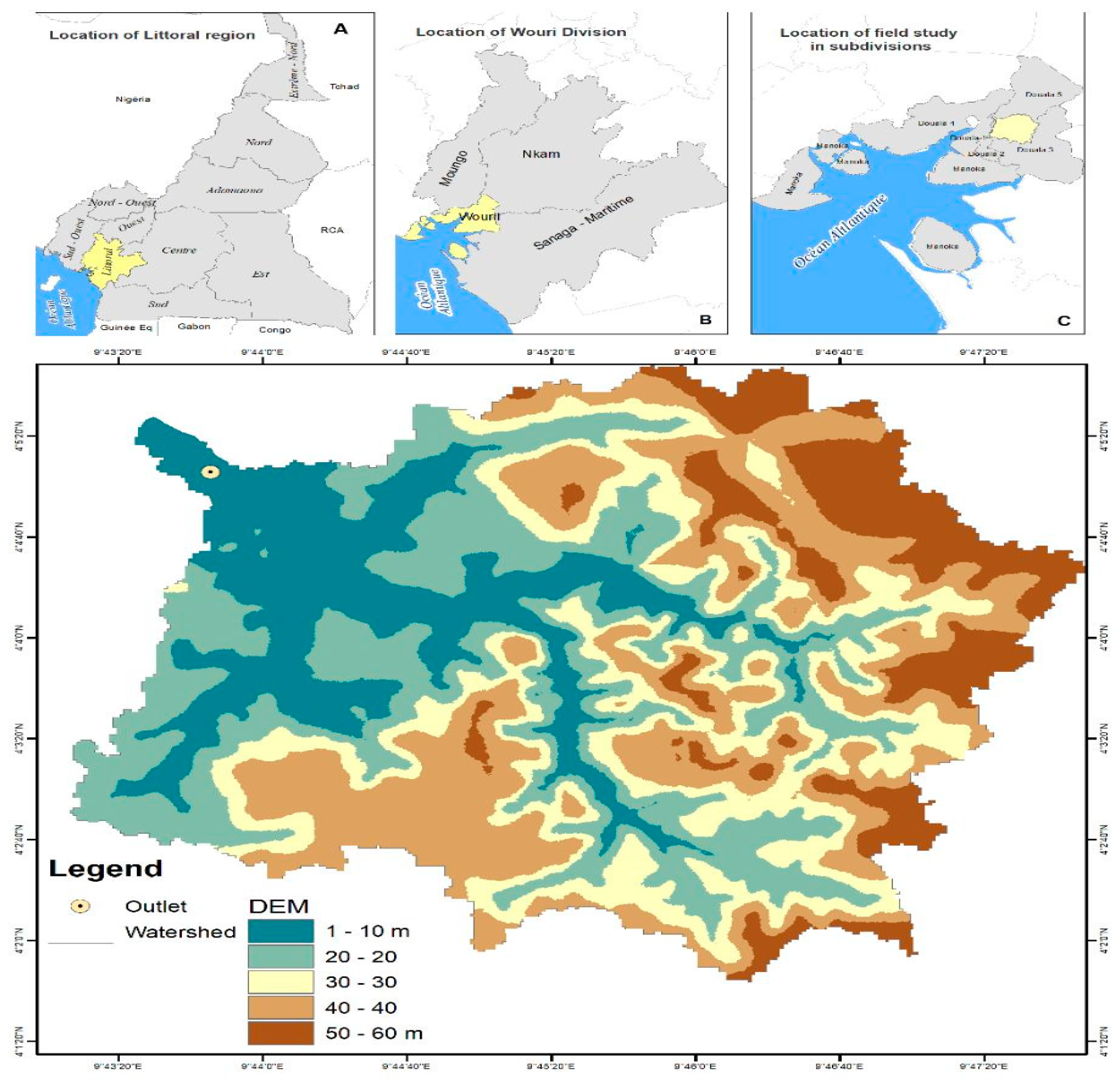
Douala is the most populous city in Cameroon, with about 3 million people distributed across the 12 watersheds. Among the watersheds, the Tongo-Bassa watershed has been chosen for this study because it has been recorded as the place where enormous human and infrastructural damage has been caused by flooding each year. The Tongo Bassa watershed is located between longitude 9°46′00″ E and latitude 4°4′00″ N (WGS 84 UTM Zone 32N) and its area is estimated at 4161.6 ha (Figure 2). [42] estimated in 2009 that the watershed constituted 27 districts, with a population density ranging from 25 to more than 350 inhabitants per hectare. The watershed has a river called the “Tongo Bassa River”, which flows into the major Wouri River in the region and then joins the Atlantic Ocean [43]. The soil of the area is essentially made up of sedimentary rocks, with colors that vary from brown to black and soils that change from sandy ferritic to deep sandy clayey soils [44].

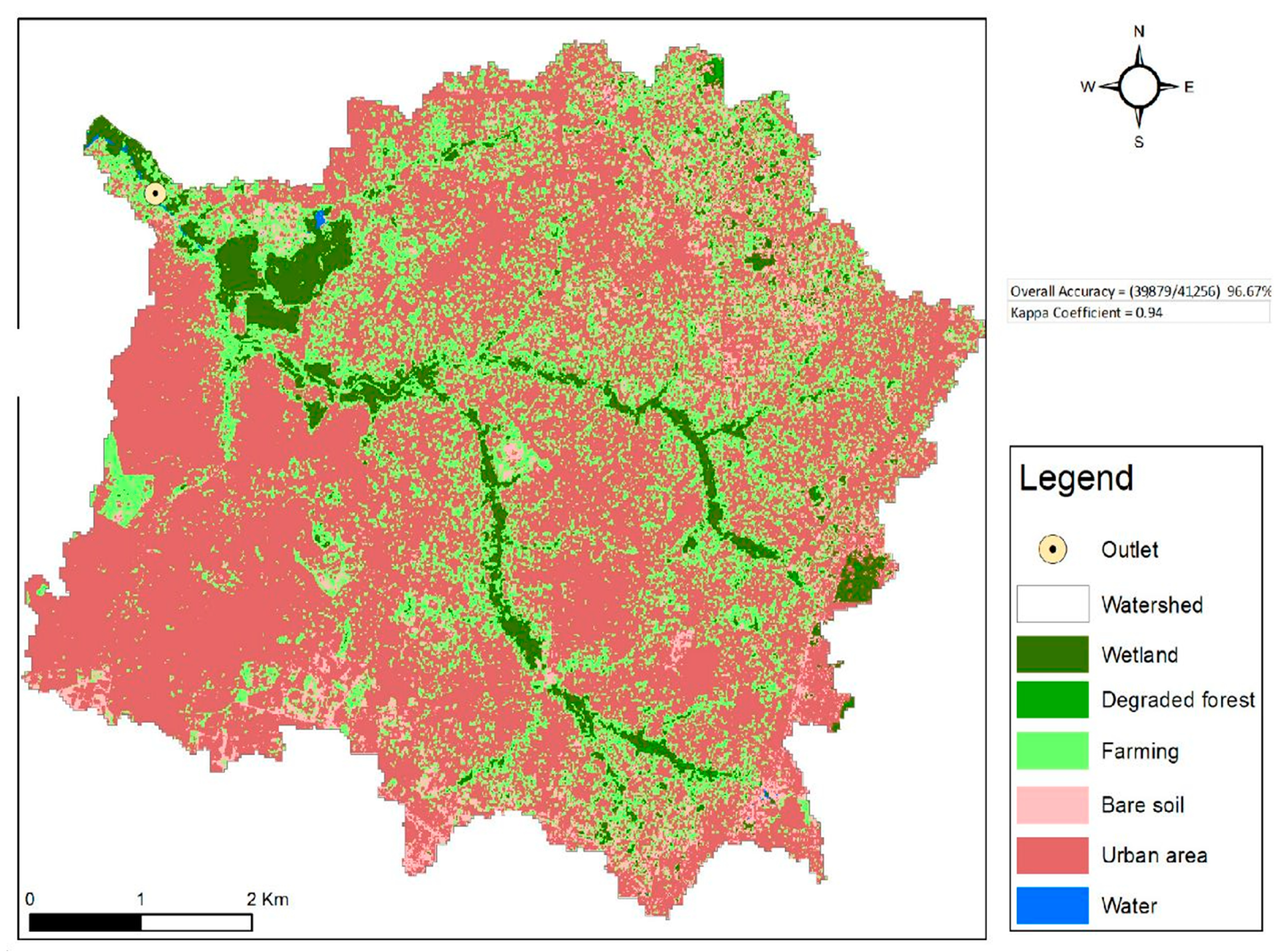
The watershed is composed of valleys where the altitudes vary from about 5 to 60 m above sea level, on average. This area is dominated by two main seasons: dry (December to February) and wet (March to November). However, it should be noted that these seasons do not affect the monthly temperatures. Particularly in August, the temperature is 26 °C and reaches 28.6 °C in February, with an annual temperature average estimated at 27 °C [45]. They found that the lowest amount of precipitation is recorded in December (the monthly average is 35 mm) and the maximum is recorded in July and August (an average of 754 mm). The land cover of the watershed is occupied by vegetated soil at 6.43% (267.61 ha), bare soil at 5.03% (209.17 ha), farming at 26.23% (1091.46 ha), urban areas at 62.25% (2590.44 ha) and water at 0.07% (2.92 ha) (Figure 3).

3.1.1. Map Processing

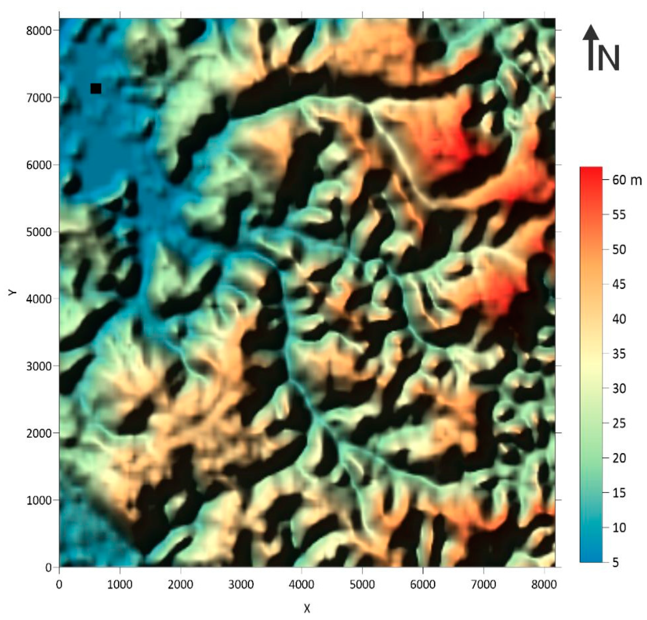
In this study, a digital elevation model (DEM) mapping 30 m from the study area was uploaded from the website (https://search.earthdata.nasa.gov/search accessed 21 June 2022) and processed using the ArcGIS software. This procedure highlighted the watershed, in addition to identifying the outlet and its coordinates; next, we imported “the whole catchment” which was previously delimited in the ArcGIS software, and the DEM uploaded using “global mapper software” for the next processing stage. The output file was created in the “xyz format”, following this final processing of the map using a global mapper with a mesh of 20 m along the x and y directions. The coordinates were output in the UTM projection and the surface was projected in a Cartesian reference frame, with a 20-meter gap in the x and y directions. The results are shown in the Figure 4, as follows.

3.1.2. Manning’s Roughness and Infiltration Parameters

We relied on the literature for sourcing data on Manning’s roughness and infiltration parameters. This is owing to the lack of relevant data in our study area. In 1989, Arcement proposed a guide for selecting Manning’s roughness coefficients for natural channels and flood plains [46].

Table 1. Infiltration parameters and Manning coefficients.

Land Cover	${\mathit{i}}_{\mathit{f}}$	${\mathit{i}}_{\mathit{o}}$	r (min−1)	n (s/m1/3)
Vegetated	0.029	0.097	1.383	0.065
Bare	0.005	0.017	1.383	0.020
Cultivated	0.021	0.069	1.383	0.050
Urban	0.003	0.008	1.383	0.015

presents the infiltration parameters proposed by [47,48], with Manning’s roughness coefficients [46].

• Sensitivity to rainfall intensity in the model

In this first case study, we used three values of rainfall intensity, as mentioned in

Table 2. The parameters applicable for the study of sensitivity to rainfall intensity.

Land Cover	${\mathit{i}}_{\mathit{f}}$	${\mathit{i}}_{\mathit{o}}$	r (min−1)	n (s/m1/3)	Rainfall Intensity (mm/h)
Vegetated	0.029	0.097	1.383	0.065	Case 1: 15 mm/h Case 2: 50 mm/h Case 2: 85 mm/h
Bare	0.005	0.017	1.383	0.020
Cultivated	0.021	0.069	1.383	0.050
Urban	0.003	0.008	1.383	0.015

.

• Sensitivity to the infiltration parameters in the model

The initial infiltration ($i_o)$, the parameters depending on the type of soil (r), and the Manning coefficient (n) were maintained as mentioned above, but only the final infiltration ($i_f)$ was subjected to several tests; i.e., 1/4$i_f$, 1/2$i_f$, 3/4$i_f,$ and $i_f$. The simulation was conducted with a rain intensity of 15 mm/h for 360 min (6 h).

4. Initial Conditions and Numerical Results

4.1. Initial Conditions

At time t = 0 s, the surface of the watershed is dry and is characterized by its topography. The velocities in the x and y directions are zero, which means u = v = 0. The watershed is traversed by a watercourse where the water height in the left and right positions is assumed to be equal to 0 m. Moreover, E and q are assumed to be 0 m³/s during the whole simulation. It is also assumed that for each part of the land used in the whole watershed, the infiltration rate and Manning coefficient are uniform and constant.

4.2. Numerical Results

4.2.1. Sensitivity to Rainfall Intensity of the Model

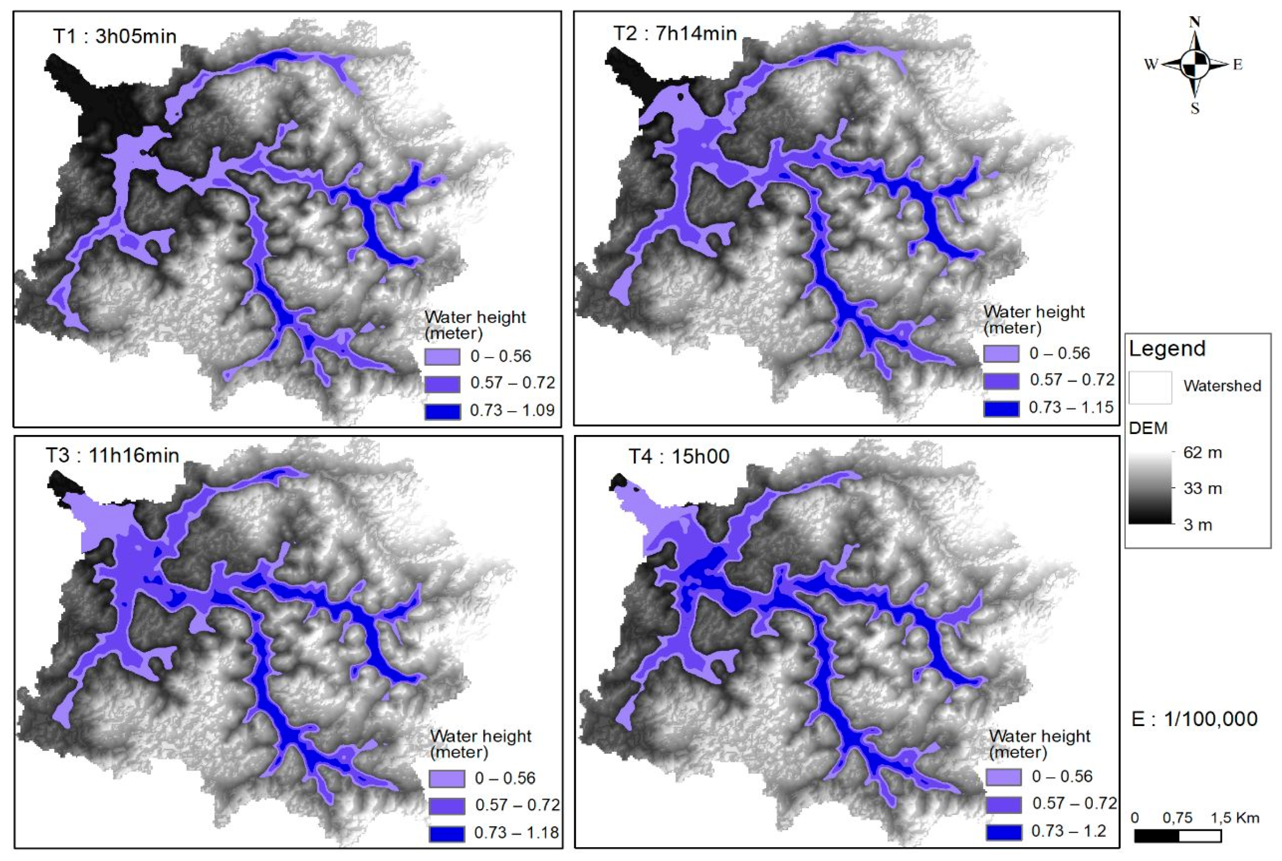
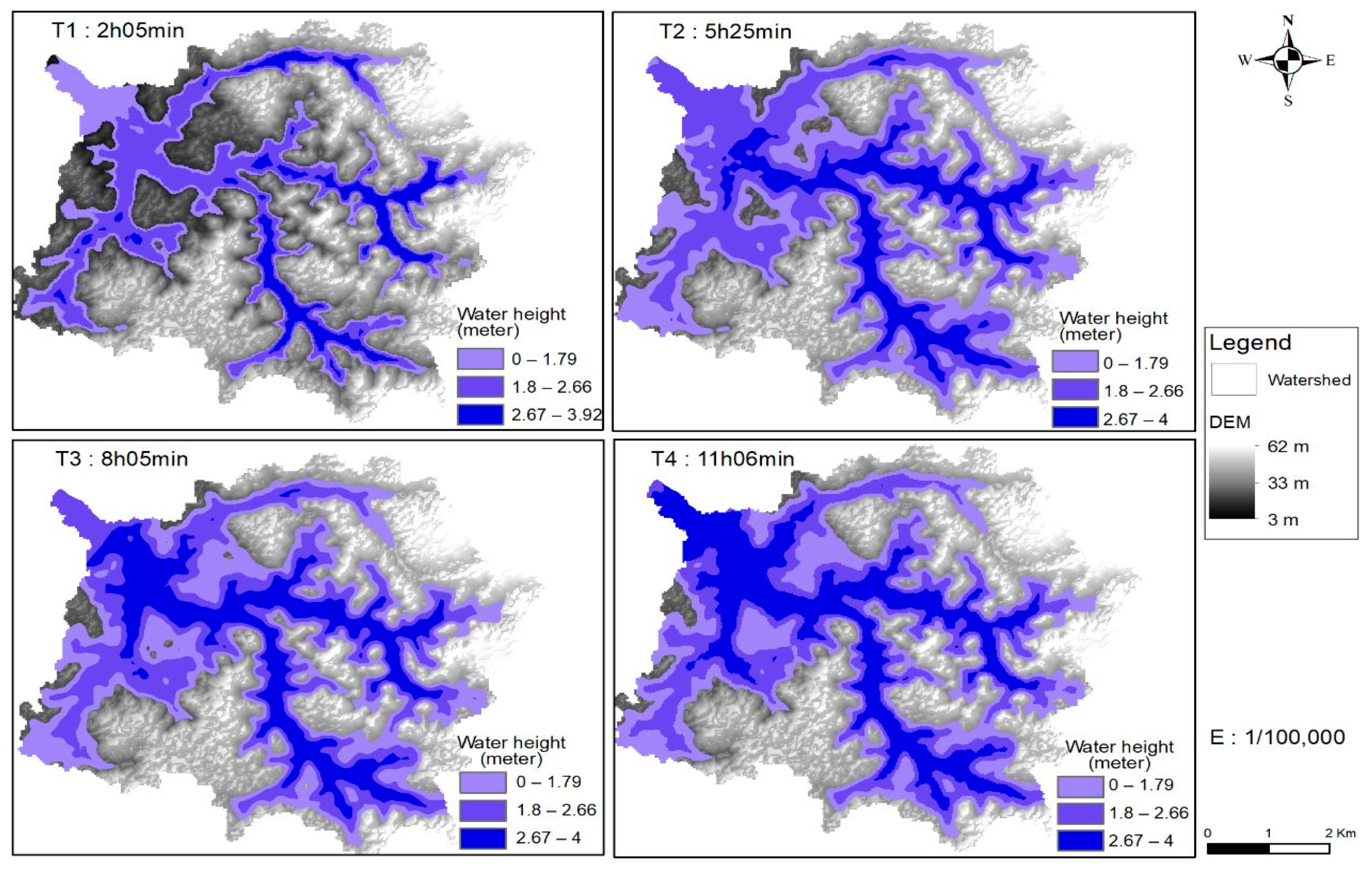
Figure 5 shows the water height propagation in the Tongo-Bassa watershed for rainfall intensity of 15 mm/h. After 15 h, a surge in the water converges toward the watercourse located in low-altitude or valley-bottom areas, which eventually comes out of its minor bed; the water height reaches 1.2 m in the deeper section.

The same simulation has been repeated, taking 85 mm/h as the rainfall intensity, and the results are illustrated in Figure 6. The distribution of water over the watershed appears greater than in case study 1 (at 15 mm/h). The floodable surface is more significant and covers the urge space of the watershed. The water heights in the lowest points (watercourse) reach a maximum value of 4 m after 11 h of simulation.

Overall, the results show that the greater the rainfall intensity, the shorter the time needed for the water in the watershed to reach a significant height. The floodable surface is well-represented in the watershed, with an emphasis on flooded areas with a wide distribution of water height.

In summary, the results indicate that water depth in the watershed is sensitive to both rainfall intensity and the simulation duration.

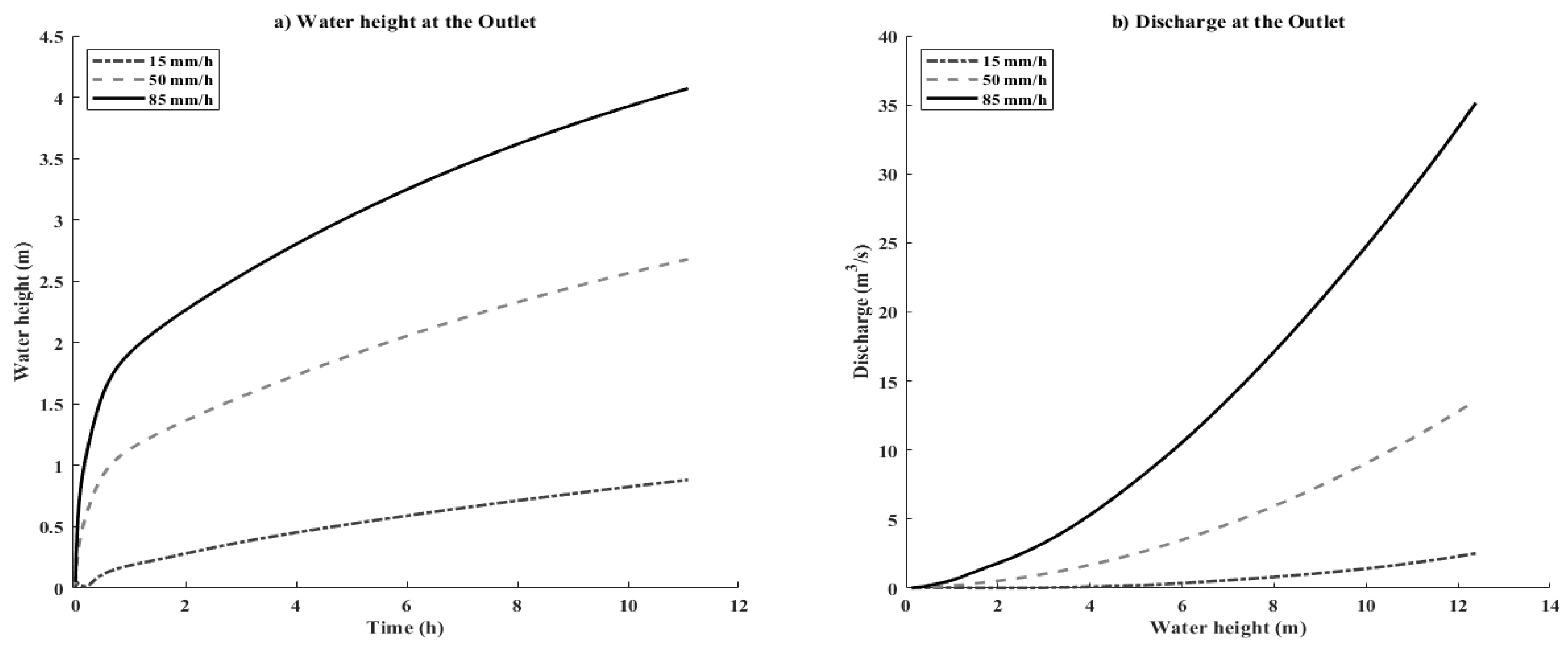
The curves presented in Figure 7a,b show the heights of the water and flow discharge obtained at the outlet for each value of rainfall intensity (15, 50, and 85 mm/h). It transpires that the height at the outlet increases with rainfall intensity and simulation duration. This can be explained by the fact that the study area is located in a sedimentary zone; the water saturation rate of the soil is very important, resulting in the low infiltration of water. The runoffs on the surface are more important and all converge toward the outlet. This explains how the greatest water depth (4.04 m) was obtained with high rainfall intensity (85 mm/h) and the lowest value (0.87 m) was obtained with low rainfall intensity (15 mm/h).

All the curves start at point 0 because it was assumed that the point located at the outlet was dry at the start of the simulation. The flow rate curves (Figure 7b) for different rainfall intensities show an increase in flow rates that is proportional to the water height. The maximum value of the flow (35 m³/s) is reached at 85 mm/h. When the rain intensity is 50 mm/h, the flow rate reaches 13.5 m³/s while at 15 mm/h, 2.5 m³/s is obtained as the maximum value of the flow at 12.14 m of water height.

4.2.2. Sensitivity of the Infiltration Parameters in the Model

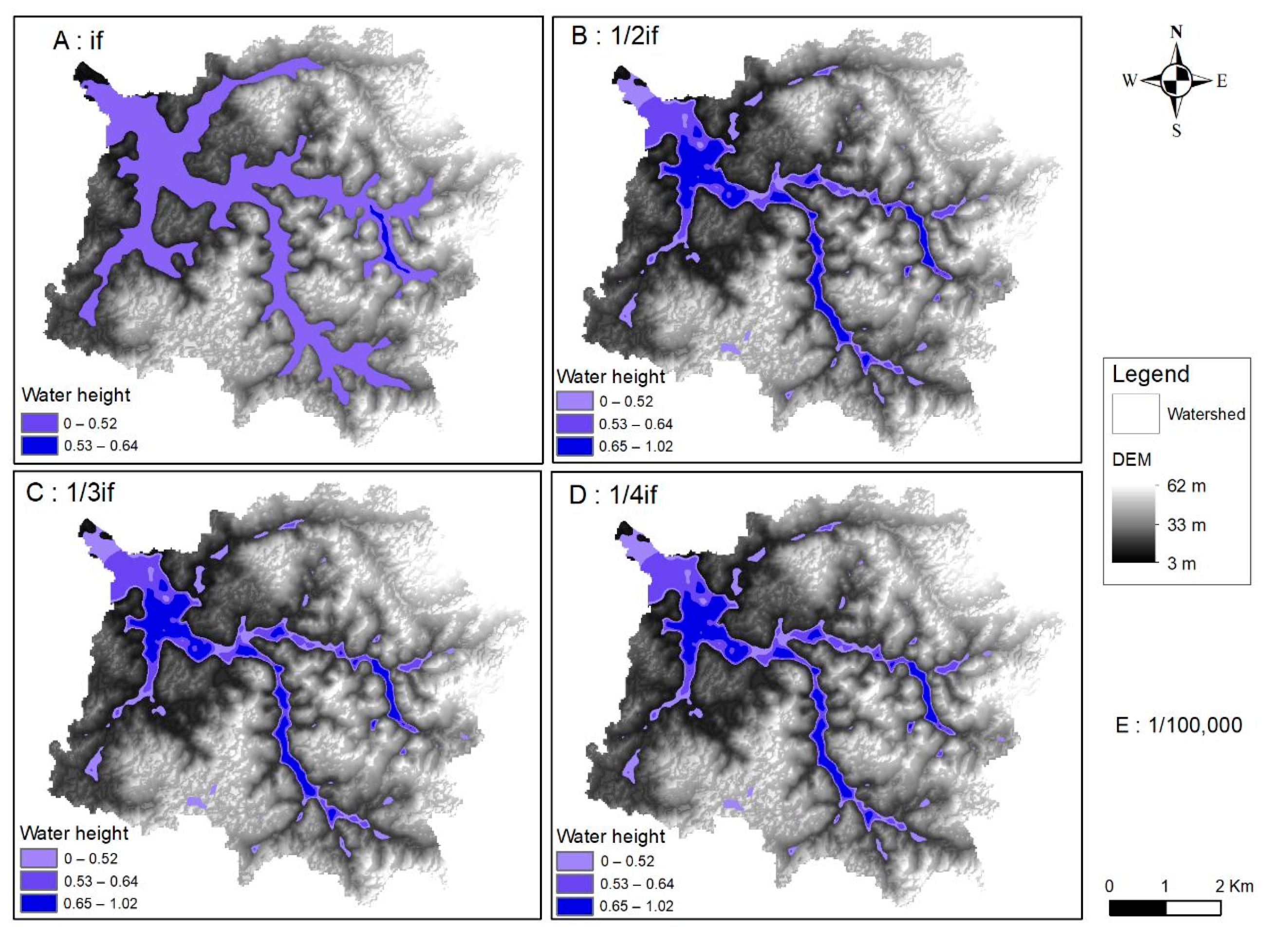
The final infiltration parameters for each case were set, as follows: 1/4i_f, 1/2i_f, 3/4i_f, and i_f; the results were obtained after 360 min (6 h). The results show that water propagation in the catchment is more significant when the final infiltration value (i_f) is high (Figure 8A). A significant quantity of the water is also flowing on the surface and toward the outlet. When the final infiltration decreases (Figure 8B–D), a large volume of water stagnates on the surface, forming small lakes where the maximum height can reach 1 m, while a very small percentage runs off to the outlet.

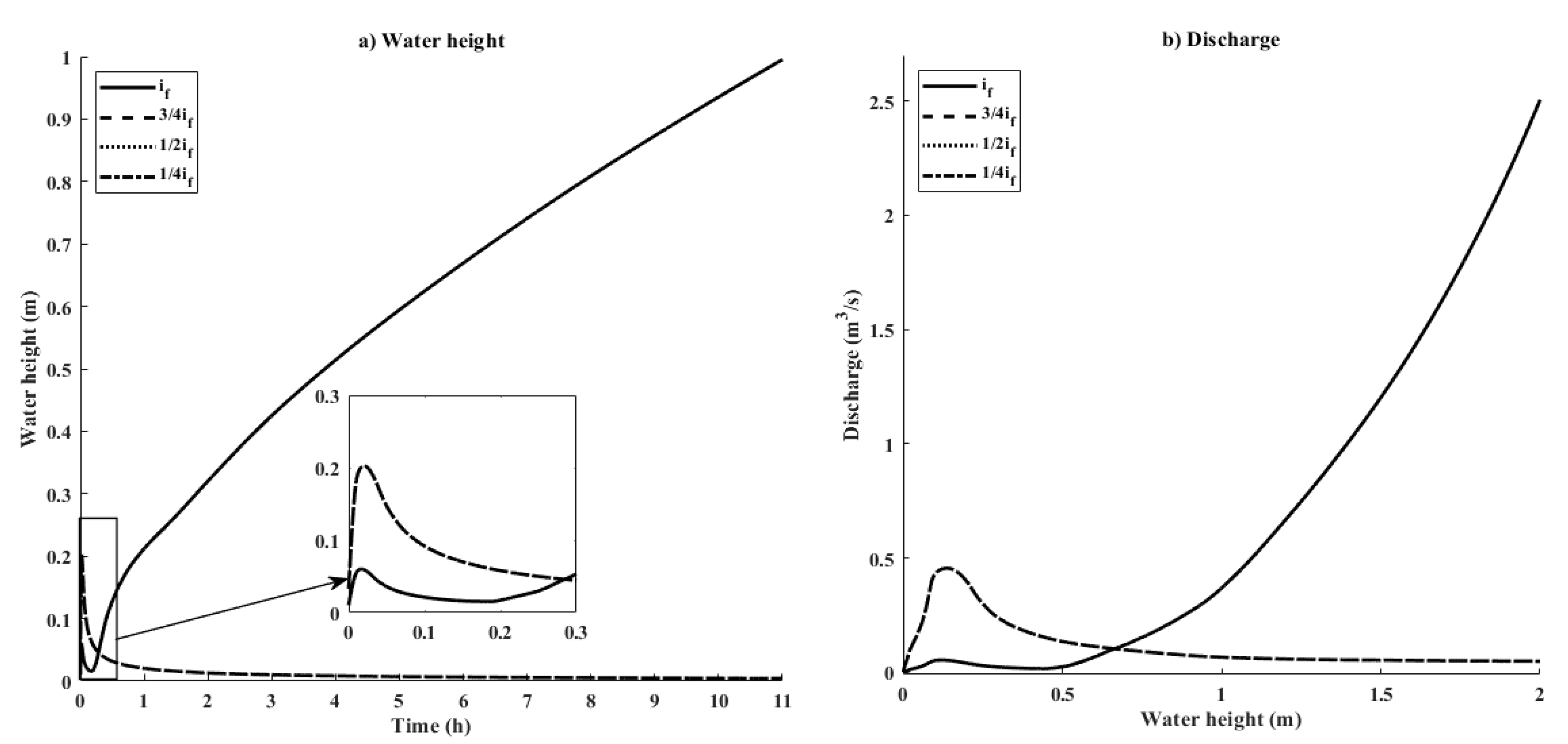
The water height and flow rates at the outlet corresponding to each final infiltration parameter are shown in Figure 9a,b, respectively. From Figure 9a, it can be seen that there is a significant difference between the curve obtained with i_f and the other curves. This shows that the maximum value of the water level is 1 m after a simulation of 11 h for (i_f), while the other curves tend toward 4.28 × 10⁻³ m. It should be noted that at the beginning of the simulation, i.e., at T = 1 min, the other curves (1/4i_f, 1/2i_f, and 3/4i_f) reach their maximum values (0.2 m); then, at the same time, the i_f curve is 0.13 m. Over a simulation time of 14 min, i.e., ranging from 0.0 to 17 min, the other curves (1/4i_f, 1/2i_f, and 3/4i_f) remain above the curve (i_f) before reversing proportionally from 17 min until the 11-hour point. This scenario supports the theory that the majority of the water stagnates on the surface and very little moves toward the outlet, which will lower the height of the water at the outlet. This same explanation is also reflected in the calculation of the rating curves in Figure 9b; the maximum flow (2.59 m³/s) is obtained with (i_f) while the rest of the curves converge toward 4.8 × 10⁻² m³/s, over a total water height at the outlet of 2 m.

4.2.3. Model Validation

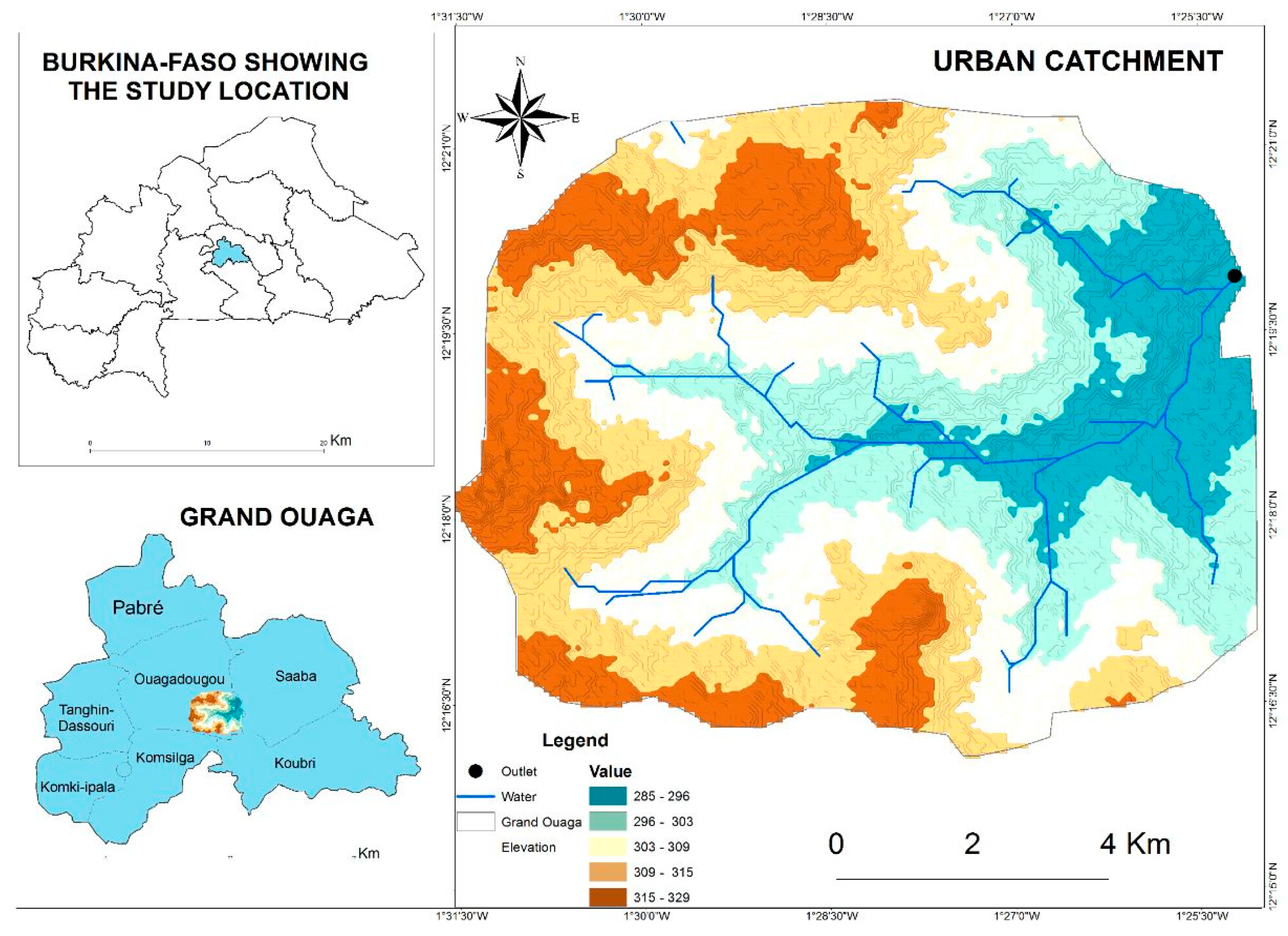
As part of the validation of the model, the Grand-Ouaga basin has been used, which is located in Burkina Faso, West Africa (Figure 10). The watershed is located between parallels 12.26° and 12.35° North in latitude and between meridians 1.43° and 1.54° West in longitude. This study is based on data from the floods that occurred in the area from 18 to 22 July 2016 (case study 1) and 25 July 2017 (case study 2). Prior to the flood, a water level gauge that allows the recording and transmission of the measurement of water height at the given point in a watercourse had been installed at the outlet. This work involved simulating the water height at the outlet, located at longitude: −1°26′ E and latitude: 12°18′ N, and comparing it to the measured data collected in the field. The mapping of the area was made according to the steps mentioned in Section 3.1 (Description of the watershed) in the current paper.

Table 3. Infiltration parameters from the Burkina Faso National Institute of Geography.

Land Cover	${\mathit{i}}_{\mathit{f}}$	${\mathit{i}}_{\mathit{o}}$	r (min−1)
Vegetated	0.22	2.95	0.503
Bare	0.54	3.46	0.116
Cultivated	0.66	4.07	0.097
Urban	0.25	3.15	0.238

presents the infiltration parameters provided by the Burkina Faso National Institute of Geography (http://www.igb.bf/ accessed on 18 January 2018).

The rainfall data used in the case study were collected from project activities (https://www.amma2050.org/ 18 to 22 July 2016; 25 July 2017).

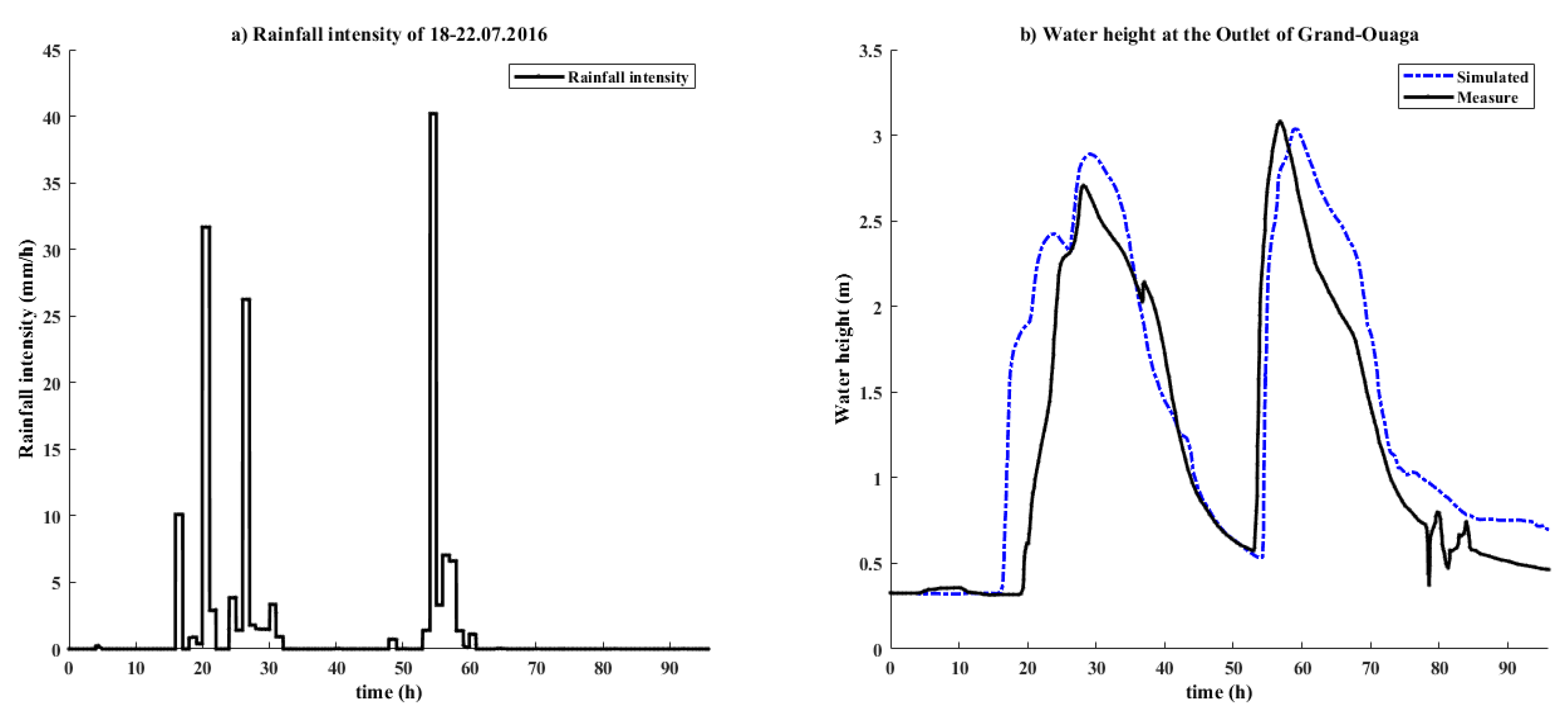
The results are presented in Figure 11a and Figure 12a for case study 1 and case study 2, respectively, and the Manning coefficients were taken [49]. At the beginning of the long rains from 18 to 22 July 2016, the water height at the outlet was estimated to be 0.32 m, while on 25 July 2017, the water height was 0 m. The comparison made between the simulated water height and the measured height is illustrated in Figure 11b and Figure 12b, for case 1 and case 2, respectively. The first comparison conducted for case study 1 (Figure 11a) over 24 h suggests a large difference in the maximum value between the observed data (2.21 m) and the simulated data (1.9 m). The Nash–Sutcliffe value is 0.7, which means a good correlation was observed between the two curves at the beginning and the end of the simulation.

According to the simulation results for case study 2 (Figure 12a), the water reaches its maximum height on the third day (of 4 days) of 3.02 m for the observed values and 3 m for the simulated values. Although the values differ somewhat, the two curves exhibit a nearly identical trend, and the Nash–Sutcliffe value is 0.73. Nevertheless, the findings show a strong link between the two trends.

The results from this validation show that the model can simulate the water height at the outlet when the coordinate points are known. The differences observed on the curves of the simulated and measured results are due to certain assumptions, such as the consideration of infiltration parameters and Manning coefficient as constant values over all the land cover. Furthermore, the digital elevation models available for free are long-dated and are not frequently updated according to the evolution of land use. In addition, these maps are downloaded with an elevation of 30 m (DEM30), which does not allow the exact land cover estimation to be established with precision.

5. Conclusions

This study applied the FVM-Godunov model to solve 2D shallow-water equations, in order to simulate the surface flow. The ghost-cell approach was integrated into the model, in order to maintain a uniform solution in both the interior and boundary cells. The model is demonstrated by simulating the surface runoff on a given catchment, by considering parameters such as infiltration, the roughness coefficient, and the rainfall intensity. The computed results were validated with the observed data on the catchment of Grand-Ouaga in Burkina Faso. The main conclusions are as follows:

• The model adapts to both the topography and the field data. The model is sensitive to several parameters, including infiltration rate, rainfall, and surface slopes. Furthermore, the model can predict the flow propagation on a given catchment and provide the water height/discharge at the outlet. As expected, runoff intensity increases with rainfall intensity, but this is not in a linear fashion; more intense rainfall produces proportionally more severe flooding.
• When the estimated final value infiltration is moderated, there is an increase in the rate of water infiltration in the catchment, which reduces the quantity of water that converges toward the outlet. This leads to a decrease in surface runoff; water tends to accumulate in the already saturated zone.
• The results proposed in the validation section show good agreement between the measured data and the simulated model. These results reveal that the parameters collected on the field and the rainfall intensity registered with the rain gauge present the results close to reality. However, it was acknowledged that the study needs improvement, which can help the model to simulate values closer to the observed values.
• The consideration of a constant and uniform value of the infiltration coefficient and the Manning coefficients in each land-cover type of the watershed also increases the risk of overestimating the results, since these different coefficients should not be considered constant. Hence, there is a need to take samples in the field with the appropriate equipment.
• Further elaboration of the model is required. For example, parameters such as evaporation, evapotranspiration, and water flow rate that are present in the study area will be considered in a subsequent study in order to improve the reach and accuracy of the final results. Although these parameters have been integrated into the numerical equations in this paper, their effects have yet to be analyzed.

References

1. Berggren, K.; Olofsson, M.; Viklander, M.; Svensson, G.; Gustafsson, A.-M. Hydraulic impacts on urban drainage systems due to changes in rainfall caused by climatic change. J. Hydrol. Eng. 2011, 17, 92–98. [Google Scholar] [CrossRef]
2. Jacobson, C.R. Identification and quantification of the hydrological impacts of imperviousness in urban catchments: A review. J. Environ. Manag. 2011, 92, 1438–1448. [Google Scholar] [CrossRef] [PubMed]
3. Fletcher, T.; Andrieu, H.; Hamel, P. Understanding, management and modelling of urban hydrology and its consequences for receiving waters: A state of the art. Adv. Water Resour. 2013, 51, 261–279. [Google Scholar] [CrossRef]
4. Semadeni-Davies, A.; Hernebring, C.; Svensson, G.; Gustafsson, L.-G. The impacts of climate change and urbanization on drainage in Helsingborg, Sweden: Combined sewer system. J. Hydrol. 2008, 350, 100–113. [Google Scholar] [CrossRef]
5. United Nations Development program (UNDP). Adapting to the Inevitable: National Action and International Cooperation; Human Development Report: New York, NY, USA, 2007; p. 36. Available online: http://hdr.undp.org/sites/default/files/hdr_20072008_fr.pdf (accessed on 10 October 2022).
6. Descroix, L.; Guichard, F.; Grippa, M.; Lambert, L.; Panthou, G.; Mahé, G.; Gal, L.; Dardel, C.; Quantin, G.; Kergoat, L.; et al. Evolution of surface hydrology in the Sahelo-Sudanian strip: An updated review. Water 2018, 10, 748. [Google Scholar] [CrossRef] [Green Version]
7. National Institution for Transforming India (NITI) Aayog. Report of the Committee Constituted for Formulation of Strategy for Flood Management Works in Entire Country and River Management Activities and Works Related to Border Areas (2021–26); Rajiv Kumar: New Delhi, India, 2021. Available online: https://www.niti.gov.in/sites/default/files/2021-03/Flood-Report.pdf (accessed on 10 October 2022).
8. IGPCC. Climate Change 2007: Synthesis Report; IPCC: Geneva, Switzerland, 2007; p. 114. Available online: https://www.ipcc.ch/site/assets/uploads/2018/02/ar4_syr_fr.pdf (accessed on 10 October 2022).
9. van den Honert, R.C.; McAneney, J. The 2011 Brisbane Floods: Causes, Impacts and Implications. Water 2012, 3, 1149–1173. [Google Scholar] [CrossRef] [Green Version]
10. Pitt, M. The Pitt Review: Learning Lessons from the 2007 Floods; The Cabinet Office: London, UK, 2008. [Google Scholar]
11. Benfield, A. Thailand Floods Event Recap Report 2011; Impact Forecasting, Report; Wiley: Chicago, IL, USA, 2012; pp. 4–40. Available online: http://thoughtleadership.aonbenfield.com/Documents/20120314_impact_forecasting_thailand_flood_event_recap.pdf (accessed on 1 March 2012).
12. Mississippi River Commission. MR & T Flood Report; Mississippi River Commission: Vicksburg, MS, USA, 2011. [Google Scholar]
13. Petrucci, O.; Pasqua, A.A.; Polemio, M. Flash flood occurrences since the 17th century in steep drainage basins in southern Italy. Environ. Manag. 2012, 50, 807–818. [Google Scholar] [CrossRef] [PubMed] [Green Version]
14. Erpicum, S.; Dewals, B.; Archambeau, P.; Detrembleur, S.; Pirotton, M. Detailed 2D numerical modeling for flood extension forecasting. In Proceedings of the 4th International Conference on Fluvial Hydraulics, Izmir, Turkey, 3–5 September 2008. [Google Scholar]
15. Okyere, C.Y.; Yacouba, Y.; Gilgenbach, D. The problem of annual occurrences of floods in Accra: An integration of hydrological, economic and political perspectives. Theor. Empir. Res. Urban Manag. 2013, 8, 45–79. [Google Scholar]
16. Garcıa-Navarro, P.; Brufau, P.; Burguete, J.; Murillo, J. The shallow water equations: An example of hyperbolic system. Monogr. Real Acad. Cienc. Zaragoza. 2008, 31, 89–119. [Google Scholar]
17. Saint-Venant, A.B. Theory and General Equations of the Non-Permanent Movement of Running Waters; Reports of the Sessions of the Academy of Sciences: Paris, France, 1871; Volume 17, pp. 147–154. [Google Scholar]
18. Li, L.; Cargnelutti, M.; Mosca, C. Dam-break flood forecasting in Piemonte region, northwest Italy. Water Resour. Manag. 1991, 5, 261–270. [Google Scholar] [CrossRef]
19. Yanmaz, A.M.; Seckiner, G.; OZaydın, V. A method for optimum layout design of concrete gravity dams. Water Eng. Res. Int. J. Korea Water Res. 2001, 2, 199–207. [Google Scholar]
20. Petaccia, G.; Natale, L.; Savi, F. Simulation of the Sella Zerbino catastrophic Dam Break. In River Flow; Proceedings of the International Conference on Fluvial Hydraulics, Izmir, Turkey, 3–5 September 2008; Kubaba Congress Department and Travel Services: Ankara, Turkey, 2008; Volume 1, pp. 601–608. [Google Scholar]
21. Bozkus, Z. Failure Analysis for Cinarcik Dam. In Proceedings of the IV National Water Engineering Symposium, Istanbul, Turkey, 6–10 July 2009; pp. 89–98. (In Turkish). [Google Scholar]
22. Tsakiris, G.; Spilliotis, M. Dam-Breach Hydrograph Modelling: An Innovative Semi-Analytical Approach. Water Resour. Manag. 2013, 27, 1751–1762. [Google Scholar] [CrossRef]
23. Brufau, P.; Vazquez-Cendon, M.E.; Garcia-Navarro, P. A numerical model for flooding and drying of irregular domains. Int. J. Numer. Methods Fluids 2002, 39, 247–275. [Google Scholar] [CrossRef]
24. Singh, J.; Altinakar, M.S.; Ding, Y. Two-Dimensional Numerical Modeling of Dam-Break Flows over Natural Terrain Using a Central Explicit Scheme. Adv. Water Resour. 2011, 34, 1366–1375. [Google Scholar] [CrossRef]
25. Mahdizadeh, H.; Stansby, P.K.; Rogers, B.D. Flood wave modeling based on a two-dimensional modified wave propagation algorithm coupled to a full-pipe network solver. J. Hydraul. Eng. 2012, 138, 247–259. [Google Scholar] [CrossRef]
26. Chen, A.S.; Hsu, M.H.; Chen, T.S.; Chang, T.I. An integrated evacuation model for highly developed urban areas. Water Sci. Technol. 2005, 51, 221–229. [Google Scholar] [CrossRef] [Green Version]
27. Alcrudo, F.; Mulet, J. Description of the Tous Dam break case study (Spain). J. Hydraul. Res. 2007, 45, 45–57. [Google Scholar] [CrossRef]
28. Mignot, E.; Paquier, A.; Haider, S. Modelling floods in a dense urban area using 2D shallow water equations. J. Hydrol. 2006, 321, 186–199. [Google Scholar] [CrossRef] [Green Version]
29. Bellos, V.; Tsakiris, G. Comparing various methods of building representation for 2D flood modeling in built-up areas. Water Resour. Manag. 2015, 29, 379–397. [Google Scholar] [CrossRef]
30. Gharbi, M.; Soualmia, A.; Dartus, D.; Masbernat, L. Comparison of 1D and 2D hydraulic Models for Floods Simulation on the Medjerda Riverin Tunisia. J. Mater. Environ. Sci. 2016, 7, 3017–3026. [Google Scholar]
31. Yung, C.Y.; Che, L.H.; Hung, S.J.; Chih, C.H.; Wei, C.B.; Yi-Chiang, Y.; Ray, S.W.; Lee-Yaw, L. An Operational Forecasting System for Flash Floods in Mountainous Areas in Taiwan. Water 2019, 11, 2100. [Google Scholar]
32. Wei-Bo, C.; Tzu-Yin, C.; Hongey, C.; Huei-Shuin, F.; Yi-Chiang, Y.; Wen-Ray, S.; Lee-Yaw, L. An Operational High-Performance Forecasting System for City-Scale Pluvial Flash Floods in the Southwestern Plain Areas of Taiwan. Water 2021, 13, 405. [Google Scholar]
33. Benedini, M.; Tsakiris, G. Water Quality Modelling for Rivers and Streams; Springer: New York, NY, USA, 2013. [Google Scholar]
34. Bahtiar, S.; Chuai-Aree, S.; Busaman, A. A numerical algorithm and Visualization Software for Flood simulation in Urban Area: A Case Study of West Jakarta, Indonesia. Int. J. Circuits Syst. Signal Proc. 2018, 12, 147–153. Available online: https://www.naun.org/main/NAUN/circuitssystemssignal/2018/a422005-aej.pdf (accessed on 10 October 2022).
35. Yamaguchi, S.T.; Ikeda, I. Rapid Flood Simulation Software for Personal Computer with Dynamic Domain Defining Method. In Proceedings of the 4th International Symposium of Flood Defense: Managing Flood Risk, Reliability and Vulnerability, Toronto, ON, Canada, 6–8 May 2008. [Google Scholar]
36. Zhou, L.; Wang, H.; Liu, D.; Ma, J.; Wang, P.; Xia, L. A second-order Finite Volume Method for pipe flow with column. J. Hydro-environ. Res. 2017, 17, 47–55. [Google Scholar] [CrossRef]
37. Maugeri, A. Capabilities of a Coupled 1D/2D Model for Flood Inundation Simulation; Columbia Water Center: New York, NY, USA, 2012. [Google Scholar]
38. Audusse, E. Hyperbolic Models and Numerical Analysis for Shallow Water Flows. Doctoral Thesis, Pierre and Marie Curie University, Paris, France, 2004. [Google Scholar]
39. Gnenakantanhan, C.; Babacar, L.; Fowe, T.; Adjadi, M.L.; Harouna, K. Urban Flood Modeling Using 2D Shallow-Water Equations in Ouagadougou, Burkina Faso. Water 2020, 12, 2120. [Google Scholar] [CrossRef]
40. Toro, E.F. The HLL and HLLC Riemann Solvers. In Riemann Solvers and Numerical Methods for Fluid Dynamics; Springer: Berlin/Heidelberg, Germany, 2009; pp. 315–344. [Google Scholar]
41. Nash, J.A.; Sutcliffe, J.V. River flow forecasting through conceptual models, I: A discussion of principles. J. Hydrol. 1970, 10, 398–409. [Google Scholar] [CrossRef]
42. Kannan, N.; Sabu, J. Quality of Groundwater in shallow Aquifers of a Paddy Dominated Agricultural River Basin, Kerala, India. World Acad. Sci. Eng. Technol. 2009, 3, 1137–1155. [Google Scholar]
43. Ministry of Urban Planning and Housing of Cameroon (MUPHC). Urban Development and Poverty reduction Strategy: City of Douala and its Greater Urban Area. Final Report, December 2009, 0828 Rapport CDS final-141209-15.12.09-JG. Available online: https://knowledge-uclga.org/IMG/pdf/development_strategy_of_the_city_of_douala_and_its_metropolitan_area.pdf (accessed on 10 October 2022).
44. Regnoult, M. Geological Synthesis of Cameroon; DMG: Yaounde, Cameroon, 1986. [Google Scholar]
45. Nkot, S.; Ketchemen-Tandia, B.; Ndje, Y.; Emvouttou, H.; Ebonji, C.R.; Frederic, H. Origin of Mineralization of Groundwater in the Tongo Bassa Watershed (Douala-Cameroon). Res. J. Environ. Sci. 2015, 7, 29–41. Available online: https://www.researchgate.net/publication/332778338_Origin_of_Mineralization_of_Groundwater_in_the_Tongo_Bassa_Watershed_Douala-Cameroon (accessed on 10 October 2022). [CrossRef]
46. Arcement, G.J.; Schneider, V.R. Guide for Selecting Manning’s Roughness Coefficients for Natural Channels and Flood Plains; US Geological Survey: Reston, VA, USA, 1989. [Google Scholar]
47. Pit, R.; Lantrip, J.; Harrison, R.; Henry, C.L.; Xue, D. Infiltration through Disturbed Urban Soils and Compost-Amended Soil Effects on Runoff Quality and Quantity; National Risk Management Research Laboratory: Duluth, GA, USA, 1999. [Google Scholar]
48. Hingray, B.; Picouet, C.; Musy, A. Hydrologie. A Science for the Engineer, 2nd ed.; PPUR Polytechnics and Universities Press: Lausanne, Switzerland, 2009; Volume 21. [Google Scholar]
49. Vidal, J.P. Assistance with the calibration of numerical models in river hydraulics—Contributions of artificial intelligence. Ph.D. Thesis, The National Polytechnic Institute of Toulouse-France, Toulouse, France, 2005. [Google Scholar]
Figure 1. The structured mesh.
Applsci 12 11622 g001
Figure 2. Location of the Tongo Bassa watershed in Cameroon: (A) (Location of Littoral Region on the Cameroon map), (B) (Location of Wouri Division on the Littoral Region), (C) (Location of Field study in subdivisons of Wouri) and Tongo Bassa Watershed.
Applsci 12 11622 g002
Figure 3. Tongo Bassa watershed land-cover map.
Applsci 12 11622 g003
Figure 4. A visualization of the watershed in an orthonormal frame.
Applsci 12 11622 g004
Figure 5. Water height propagation at different time steps for a constant rainfall intensity (15 mm/h).
Applsci 12 11622 g005
Figure 6. Water-height propagation at different time steps for a rainfall intensity of 85 mm/h.
Applsci 12 11622 g006
Figure 7. Water height (a) and discharge (b) at the outlet.
Applsci 12 11622 g007
Figure 8. Water height propagation map after 6 h, with 15 mm/h as the rainfall intensity.
Applsci 12 11622 g008
Figure 9. Water height (a) and flow rates (b) at the outlet of the catchment for different values of final infiltration, with 15 mm/h set as the rainfall intensity.
Applsci 12 11622 g009
Figure 10. Location map of the Grand-Ouaga area in Burkina Faso (West Africa).
Applsci 12 11622 g010
Figure 11. Rainfall intensity (a) and a comparative study of the water height (b), during the flood of 25 July 2017.
Applsci 12 11622 g011
Figure 12. Rainfall intensity (a) and comparative study of the water height (b) during the flood of 18 to 22 July 2016.
Applsci 12 11622 g012