Abstract
Most geophysical inversions face the problem of non-uniqueness, which poses a challenge in the mapping and delineation of the subsurface anomalies. To tackle this challenge, a combined local and global optimization approach is considered for jointly inverting two-dimensional direct current resistivity (DCR) and seismic refraction (SR) data that aim to estimate the corresponding physical model parameters. In this combined approach, the output of the local optimization method is used to determine the search space and tuning parameters for the global optimization algorithm. The multi-objective genetic algorithm (non-dominated sorting genetic algorithm) was utilized to jointly optimize the objective functions of two different methods. Because the genetic algorithm is a population-based optimization method, it requires numerous forward calculations. To deal with the expected high computational cost associated with this approach, parallel computing was utilized for the forward function evaluations to reduce the run time of the entire process. The proposed approach was tested using synthetic two-dimensional resistivity and velocity models that had three different types of anomalies (dyke, positive, and combined positive and negative). The results showed an improvement in the anomaly delineation in the output of the combined local and global optimization method compared with the local optimization method. Additionally, similar synthetic models were tested using only the single objective global optimization algorithm (conventional global optimization), which showed promising anomaly delineation.
1. Introduction
The primary goal of inverting geophysical data is to estimate the parameters of a model that will give a theoretical response similar to the field observations [1,2]. However, it is unusual to have a unique solution since most geophysical inverse problems are ill-posed. Previous studies included regularization constraints in the objective function to solve the problem of instability [3,4,5,6]. In some cases, with a regularization term in the objective function, the inversion still faces the challenge of non-uniqueness (i.e., ambiguity) associated with the inverse problem. To reduce uncertainties related to the inversion of a dataset belonging to a single geophysical method, many researchers have applied the concept of joint inversion [7,8,9,10,11,12,13,14,15,16] of more than one method, which provides better model resolution than individual inversion [17,18,19]. Joint inversion can even resolve ambiguity associated with the geophysical method(s) applied in an area with low physical properties contrast [20,21,22]. Geophysical joint inversion tries to optimize a single objective function formed by a weighted or arithmetic sum of the individual objective functions of corresponding methods [23]. However, the issue of parametric coupling (i.e., model integration) arises when we are dealing with the inversion of datasets acquired with more than one geophysical method [24].
In this study, we apply the structural model coupling approach, which involves the cross-gradient constraint method that is commonly used for geophysical inversion [8]. The basic idea using this approach is that the gradients of relevant model parameters are spatially correlated. The cross-gradient approach has been adapted for the joint inversion of different geophysical data [13,14,15,16,25,26,27,28,29]. Wang et al. [17] applied the cross-gradient algorithm in a joint inversion involving both the controlled-source audio magnetotelluric (CSAMT) and magnetic methods. Demirci et al. [15] formulated an objective function concerning weighted cross-gradient, which limits the dominance of one type of model parameter to another. Zhang et al. [30] utilized the cross-gradient constraint to impose a common structural framework in the joint inversion of EM and acoustic data, which reconstructs the structures satisfactorily.
Furthermore, Yin et al. [31] applied a cross-gradient technique to invert magnetotelluric (MT) and gravity data and tested their algorithm using both synthetic and real datasets. Finally, Jordi et al. [32] introduced a new approach to the cross-gradient constraint, which involved the use of an irregular grid in unstructured mesh in the finite element method. They used the method to invert the DCR and ground penetrating (GPR) data. All the above examples used the conventional or local optimization method that incorporated all acquired data within the same Jacobian using a unique objective function for all geophysical methods.
The local optimization techniques are applied iteratively to obtain an updated model that minimizes the objective function, which may not be the global solution to the inverse problem. The global optimization algorithm in geophysical inversion might be used to search for a solution space to avoid being stuck in the local minimum of the objective function. For instance, Liu et al. [33] applied the particle swarm optimization (PSO) algorithm in a parametric inversion involving magnetic data. Rani et al. [34] used the genetic price algorithm (GPA) to monitor the movement of contaminants in the subsurface. Additionally, [35] introduced a hybrid approach by using the results of the local optimization method as an input to the genetic algorithm for the modeling of the SR data. This novel algorithm by [35] overcame the problem of being stuck in the local minima. It optimized the computational cost of the genetic algorithm using the multicore parallel computing method.
Similarly, local and global (hybrid) optimization has been applied to complement each other to subdue their shortcomings [35,36,37]. Most previous work has considered an objective function from a different perspective to perform joint inversion using a global optimization method, such as when using a local optimization algorithm. For instance, Schwarzback et al. [38] and Ayani et al. [39] considered the objective function for the inversion of electromagnetic data in two terms. First, they tried to minimize the data misfit and the roughness of the model at the same time. Akca et al. [40] applied a non-dominated sorting genetic algorithm in a joint 1D parametric inversion involving magnetic resonance and vertical electrical sounding.
In previous studies, joint inversion/interpretation was applied by using either local or global optimization methods. Moreover, local and global (hybrid) optimization has been applied to complement each other to subdue their shortcomings. However, based on our knowledge, the joint modeling of different geophysical data by using the results from the inversion (local optimization) to constrain the search space of the global optimization approach has never been reported in the literature. Thus, a procedure that constrains the global part of the combined optimization algorithm by using the local optimization to define a close search space to the real model parameters was proposed and designed. In this way, the search space of the model parameters has been limited to a more reliable range, drastically reducing the computation time.
This study presents the combined local and global optimization approach to jointly model SR and DCR data. With this proposed approach, the multi-objective (i.e., integration of the DCR and SR misfit functions) global optimization algorithm is used for the first time for the two-dimensional joint inversion of two different geophysical datasets, i.e., SR and DCR data. Specifically, in this algorithm, the global part of the combined optimization algorithm is constrained by using the output of the local optimization to define a search space, significantly improving its run time and mitigating model instability. In addition to the improved computational cost that resulted from applying the combined local and global optimization methods, we made the multi-objective global optimization algorithm run on parallel computing. This process further optimized the computational cost and devised the optimum technique using the combined optimization algorithm. We tested and discussed the efficacy of our proposed algorithm using synthetic SR and DCR data.
2. Optimization Methods
2.1. Local Optimization Method
The individual and joint inversion of DCR and SR data are usually regularized with a smoothing function due to the non-uniqueness and instability associated with the inverse process. In the inversion of both DCR and SR methods, the data misfit can be formulated as follows:
f(m) is a function that is used to describe forward modeling, is the observed field record, and is the weight matrix used to adjust the data anomaly (e.g., high or low amplitudes). Usually, we use norms to quantify the misfit between the observed and calculated data, and the common one used for this type of inverse problem is the L2 norm because we assume that the error in the data is Gaussian. Therefore, the objective functions for the DCR and SR data are given as follows:
where is the misfit or objective function, and are the measured data, and and is the model response for the DCR and SR methods, respectively. Additionally, is the Laplacian of the model parameter that is transformed into the smoothness matrix by obtaining its Laplacian operator, while and are the regularization parameters that determine the level of the smoothness of resistivity and seismic models, respectively. The joint inversion offers conventional ways of integrating data from different geophysical methods in such a manner that the outcome models are consistent and similar. One of the methods used to accomplish this goal is to apply the cross-gradient constraint proposed by Gallardo et al. [8] in the objective function. The parallel spatial variation in the models (resistivity or seismic velocity) is required to satisfy the cross-gradient constraint [8,13,15]. This means that model anomalies or layer boundaries must essentially point in the same or opposite direction. Applying the cross-gradient constraint, Equations (2) and (3) become:
subject to . Where is the cross-gradient constraint and can be defined as:
Equation (4) can be minimized by applying the appropriate regularized local optimization algorithm similar to the approach used in [15]. Therefore, the model parameter correction vector can be expressed as:
where and are defined as:
In Equations (7) and (8), is the Jacobean matrix, is the weighting matrix, is the data residual, is the Laplacian operator, and is the cross-gradient derivative. The terms given in Equations (7) and (8) may be rewritten for the joint inversion case as follows:
In this inversion approach, a resistivity model is created for the DCR method, while for the slowness model, the inverse of velocity is used for the SR method [15]. Conceptually, the joint inversion process requires the model discretization for all the geophysical methods to be structurally similar.
2.2. Global Optimization Method
The global optimization method applied in this study involves the application of the genetic algorithm (GA) for a single objective function case and non-dominated sorting genetic algorithm 2 (NSGA II) for the multi-objective joint optimization approach. The GA is a special case of evolutionary algorithm that simulates the process of biological evolution, and it is adapted to solve an optimization problem [41,42,43]. The process of the genetic algorithm starts from population initialization, which creates chromosomes (potential solutions with respect to the objective function) using the binary coding scheme. The binary coding scheme is conceptualized in a way that it constitutes a solution to the objective function of the inverse problem [43]. The binary coding system has a bit string or chromosome that describes each element or individual in the population. Each bit in the bit string represents a gene that can be assigned values of 0 or 1, also known as an allele [43]. Two individuals or parents are paired or selected from the initial population to produce two offspring. The higher the fitness value of an individual in the population, the higher the chance of being selected and the better its performance in the evolution loop. Among other selection methods, we apply the tournament selection because it practically depicts natural competition for mating rights among individuals in a population. Crossover involves exchanging information (genetic properties) between two paired models (parents) to create two new models (offspring). Three types of crossover options are available in the code used in this study: single point, two points, and scattered crossover. The final evolution operator used in the genetic algorithm is the mutation. This is the random alteration of genes in a chromosome to introduce diversity in the entire population of the genetic algorithm. This process is usually conducted using a probability index that is appropriately chosen based on the degree of randomness to be allowed and computation cost. The process described above is generally referred to as a single objective genetic algorithm; it is suitable for the inverse problem having one objective function (i.e., applied in the individual inversion of DCR or SR). All these GA evolution operators (i.e., selection, crossover, and mutation) are used to modify the solution parameters.
As mentioned above, the non-dominated sorting genetic algorithm 2 (NSGA II) is a variant of the GA commonly used to solve multi-objective optimization problems. The NSGA II procedures involve the creation of an offspring population () that has an equal size to the initial population () using the selection, crossover, and mutation processes as shown in Figure 1. After that, () and () are combined to produce (), which is double the size of (). Then, the non-domination (i.e., the optimum set of solutions in all the objective functions) sorting of the entire population () is performed, and the best non-dominated solutions are selected, which are indicated as (levels of non-domination) in Figure 1. The topmost non-dominated solutions are accepted until the initial population size is reached; thereafter, the rest of the non-dominated solutions are rejected because the process cannot accept more than the initial population size. Sometimes only can satisfy the initial population size requirement, and that will be enough for the next generation (); then, the rest are rejected (Figure 1). Consequently, the NSGA-II emphasizes both the non-dominated and less crowded points.
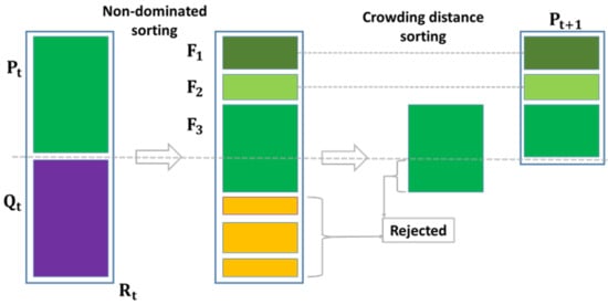
Figure 1.
Illustration of the non-dominated sorting algorithm 2 (NSGA II). Qt is the offspring population; Pt is the initial population; Rt is the total population; and F1, F2, and F3 are the levels of non-domination solutions.
One of the major challenges in applying the genetic algorithm to the inverse problems that require the simultaneous optimization of more than one objective function is preventing the domination of one objective function to another. Therefore, the multi-objective genetic algorithm was used to search for the optimum solutions that do not dominate (i.e., a set of optimum solutions in both DCR and SR objective functions) each other. The two objectives of the joint inversion of DCR and SR data using the multi-objective global optimization method can be represented similar to Equation (1) as:
and
The objective functions are used to map the decision variables (model parameters) into an objective space where we delineate solutions that are not dominated or perform optimally in both objectives. These sets of solutions (Pareto sets) align in a pattern known as Pareto optimal solutions or the Pareto front [44]. Basically, the term “Pareto optimality” is used to describe these sets of solutions, implying that no further optimal solution in both objectives can be obtained. Details about the concept of Pareto optimality and non-domination is discussed by [12]. The NSGA II algorithm sorts the set of solutions as they arrive at the Pareto optimal front. This technique was proposed by [45] to overcome some of the limitations observed in some previous evolutionary multi-objective algorithms. These limitations include computational intricacy, elitism problems, and parameter sharing specifications. The NSGA II only utilizes standard parameters of the genetic algorithm needs, and no extra parameters are needed for its multi-objective base optimization (see the appendix section for the concept of NSGA II).
2.3. Combined Local and Global Optimization Method
In the combined optimization algorithm, we used the output of the local optimization method to define the search space for the global optimization technique to speed up and reach the global solution faster. Since the local optimization has been constrained by smoothing terms (i.e., second terms of Equations (2) and (3)), the combined optimization algorithm is linearly constrained by applying the output of the local optimization algorithm to define the lower and upper bounds of the search space. Fundamentally, the search space is determined by modifying the range (minimum and maximum) of the model parameters obtained from the output of the local optimization algorithm. Depending on the quality of the output from the local optimization algorithm, scaling the model parameters up and down by 10 to 30% is recommended to obtain a good result. The variability (10–30%) of the model parameters was selected based on the expected variation in the modeled geophysical properties, such as velocity and resistivity, in Saudi Arabia. This process creates adequate diversity in the initial population for the global optimization algorithm. A flowchart illustrating the combined local and global optimization algorithm is shown in Figure 2. The summary of all terms we used to describe the combined optimization algorithms is presented in Table 1.
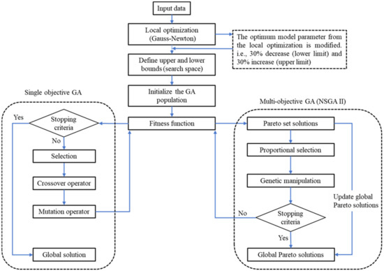
Figure 2.
Flowcharts of the proposed combined local and global optimization algorithm.

Table 1.
A summary of all the types of inversion applied in this study, their description, and abbreviations are presented below.
3. Synthetic Test
3.1. Synthetic Data
We examined the feasibility of the combined global optimization (CGO) algorithm by using synthetic earth models that simulated three near-surface scenarios. The first model comprised a dyke anomaly with a resistivity of 1250 ohm-m and a two-layered host environment with resistivities of 50 ohm-m and 250 ohm-m. Similarly, a dyke anomaly having a velocity of 2200 m/s and a two-layered host environment with layer velocities of 1000 m/s and 1500 m/s, respectively, was used for the corresponding velocity model (Figure 3a,d). The second model contained two blocks of positive anomalies, having a resistivity of 250 ohm-m and velocity of 2000 m/s, which was greater than the host environment as shown in Figure 3b,e. The third model was similar to the second one, with a higher parameter contrast (higher and lower than the host model anomalies) compared with the host rock, where the block parameters were set as 1250 ohm-m, 2500 m/s (Figure 3c,f). Generally, these models had the same profile length of 240 m in both methods, with a depth of 50 m in the DCR and 60 m in the SR methods. The DCR data were calculated for a setup with equally spaced 49 electrodes 5 m apart using the dipole–dipole (DD) array. The DD array was selected, since it had a fair penetration depth and a very good to excellent lateral resolution. The seismic survey layout was similar to the DCR profile, where we used 49 receivers with 5 m spacing and 13 sources with 20 m intervals in the SR forward calculations.
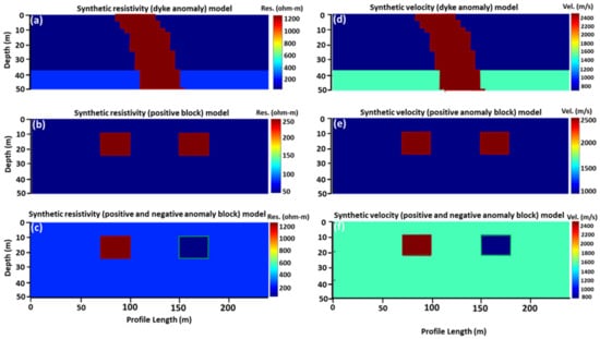
Figure 3.
Synthetic models for (a) resistivity (dyke anomaly) model, (b) resistivity (positive anomaly) model, (c) resistivity (positive and negative anomalies) model, (d) velocity (dyke anomaly) model, (e) velocity (positive anomaly) model, and (f) velocity (positive and negative anomalies) model. The dark red and green lines are used to mark the anomaly boundaries.
3.2. Synthetic Results
To obtain good local optimization (LOM) results, an appropriate regularization parameter was used in addition to adding the smoothing term in the objective function [46,47]. The regularization parameter was determined by obtaining the maximum value of the diagonal matrix in the singular value decomposition of the Jacobian matrix in both the individual and joint inversion of the DCR and SR data. The value of the regularization parameter was modified using a cooling approximation at each iteration. The inversion process started with the initial guess of the model parameters that improved with each iteration. This procedure was used to estimate the model parameter correction vector as applied by [15,16]. The LOM was terminated when there was no decrease in error and the RMS dropped below a certain threshold value (convergence criteria). In the combined global optimization (CGO) techniques, a forward modeling algorithm was used to estimate the theoretical data in both DCR and SR methods; thereafter, the calculated data were compared to the observed field data to compute their misfits. The data misfit (from Equations (10) and (11)) for the DCR method is presented in a simplified form as:
where is the observed real data, Wdc is the weighting matrix of the real data, and is the theoretical data. The misfit function for the SR method is defined with a similar annotation as:
The combined misfits form the objective function for the multi-objective optimization algorithm that is represented as:
Notice that for the multi-objective (MOO) algorithm in Equation (14), the individual misfits are not added together but are simply concatenated to make a two-column matrix of the misfits. In addition, selecting the number of populations and generations is important to improve the model resolution in the CGO algorithm for both methods. Conventionally, the population size of 50 is recommended for the GA, with the number of decision variables less than or equal to five. Otherwise, 200 populations should be used when the decision variable is greater than five. The CGO algorithm is terminated when the average change in the spread of Pareto solutions is less than the function tolerance (i.e., 1 × 10⁻⁴ for multi-objective optimization, MOO) and the specified number of generations (i.e., for single objective optimization, SOO).
The single objective genetic algorithm runs between 1000 and 1500 generations with an average population size of 250 individuals in both DC-resistivity and SR methods. The SR genetic algorithm runs were completed in about 748, 876, and 1194 min for the dyke, positive, and combined positive–negative anomalies synthetic models, respectively, while the processing times were measured as 176, 181, and 150 min for DC data. After applying the single objective (SOO) genetic algorithm in both geophysical methods (DCR and SR) separately, we performed the joint parameter estimation using the multi-objective (MOO) genetic algorithm. The non-dominated sorting genetic algorithm (NSGA II) used in the multi-objective global optimization showed that there were feasible solutions depicted by their Pareto optimal fronts (Figure 4). The compromised solution (the green star in Figure 4) was chosen and presented as the output of the MOO method. The NSGA II (for both geophysical methods) ran for about 3136, 2953, and 2891 min for the dyke, positive, and the combined positive and negative anomalies synthetic models, respectively. Figure 5, Figure 6, Figure 7, Figure 8, Figure 9 and Figure 10 show the results of the local and combined optimization methods for the dyke anomaly model (Figure 5 and Figure 6), positive anomaly (Figure 7 and Figure 8), and the positive and negative anomaly models (Figure 9 and Figure 10). The first column of each of the figures contains the inverted resistivity models, while the second column is the inverted velocity models. In addition, the first row in each figure contains the synthetic models, the second row is the individual (IIM)/single objective (SOO) inverted models, and the third row is the joint (JIM)/multi-objective (MOO) inverted models.
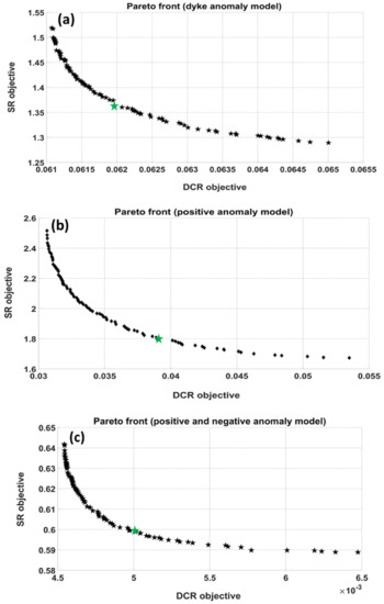
Figure 4.
Plots of the Pareto fronts showing the compromise solution (green star shape) for (a) a dyke anomaly model, (b) a positive anomaly model, and (c) positive and negative anomalies model.
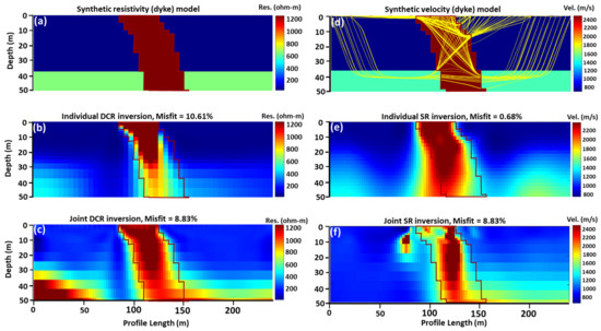
Figure 5.
Dyke anomaly model inversion using local optimization method; (a) synthetic dc-resistivity model, (b) individual inverted resistivity model, (c) joint inverted resistivity model, (d) synthetic velocity model and its ray path coverage, (e) individual inverted velocity model, (f) joint inverted velocity model. The dark red line is used to mark the anomaly boundary.
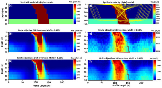
Figure 6.
Dyke anomaly model inversion using combined optimization method; (a) synthetic dc-resistivity model, (b) single objective inverted resistivity model, (c) multi-objective inverted resistivity model, (d) synthetic velocity model and its ray path coverage, (e) single objective inverted velocity model, and (f) multi-objective inverted velocity model. The dark red line is used to mark the anomaly boundary.
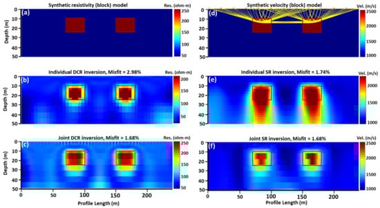
Figure 7.
Positive anomaly model inversion using local optimization method; (a) synthetic dc-resistivity model, (b) individual inverted resistivity model, (c) joint inverted resistivity model, (d) synthetic velocity model and its ray path coverage, (e) individual inverted velocity model, and (f) joint inverted velocity model. The dark red line is used to mark the anomaly boundary.
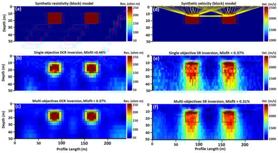
Figure 8.
Positive anomaly model inversion using combined optimization method; (a) synthetic dc-resistivity model, (b) single objective inverted resistivity model, (c) multi-objective inverted resistivity model, (d) synthetic velocity model and its ray path coverage, (e) single objective inverted velocity model, and (f) multi-objective inverted velocity model. The dark red line is used to mark the anomaly boundary.
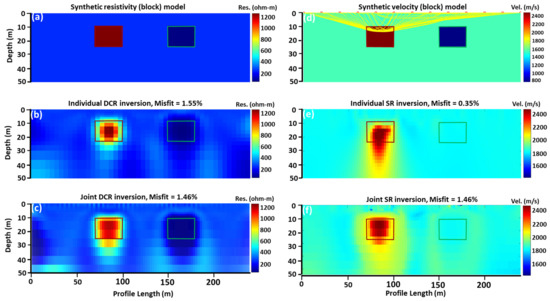
Figure 9.
Positive and negative anomaly model inversion using local optimization method; (a) synthetic dc-resistivity model, (b) individual inverted resistivity model, (c) joint inverted resistivity model, (d) synthetic velocity model and its ray path coverage, (e) individual inverted velocity model, and (f) joint inverted velocity model. The dark red and green lines are used to mark the anomaly boundary.
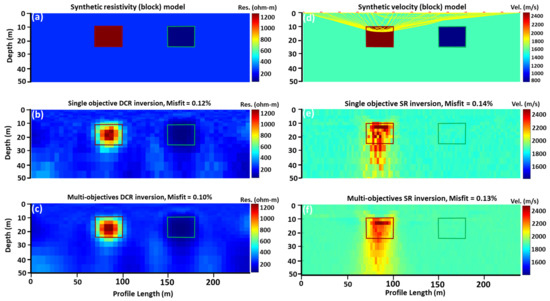
Figure 10.
Positive and negative anomaly model inversion using the combined optimization method; (a) synthetic dc-resistivity model, (b) single objective inverted resistivity model, (c) multi-objective inverted resistivity model, (d) synthetic velocity model and its ray path coverage, (e) single objective inverted velocity model, and (f) multi-objective inverted velocity model. The dark red and green lines are used to mark the anomaly boundary.
To see the performance of the conventional global optimization (GOM) only using a similar misfit function as applied in the CGO method, we applied the genetic algorithm with a search space defined apart from the local optimization results using the same DCR and SR synthetic models. Applying the single objective genetic GOM algorithm to the resistivity model showed that the GOM technique provided unstable solutions in delineating both DCR and SR anomalies. For example, Figure 11, Figure 12, Figure 13 and Figure 14 are the outputs of the genetic algorithm application on the dyke anomaly model (for both DCR and SR), the positive anomaly model, and the combined positive and negative anomaly model (for DCR only). Some of the artifacts observed in the results could probably be attributed to the absence of a constraint or model regularization [38]. The genetic algorithm was applied for 200 generations in the case of the SR method and 2500 generations for all DCR models inversion with a population size of ten times the amount of model parameters [35] in both geophysical methods. This inversion is feasible with the use of high performance and parallel computing (HPPC).
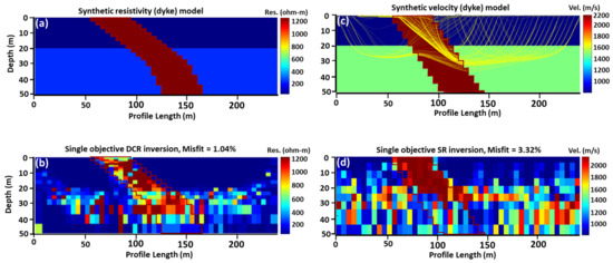
Figure 11.
Dyke anomaly model inversion using the single objective global optimization method; (a) synthetic dc-resistivity model, (b) single object inverted resistivity model, (c) synthetic velocity model, and (d) single objective inverted velocity model. The dark red line is used to mark the anomaly boundary.
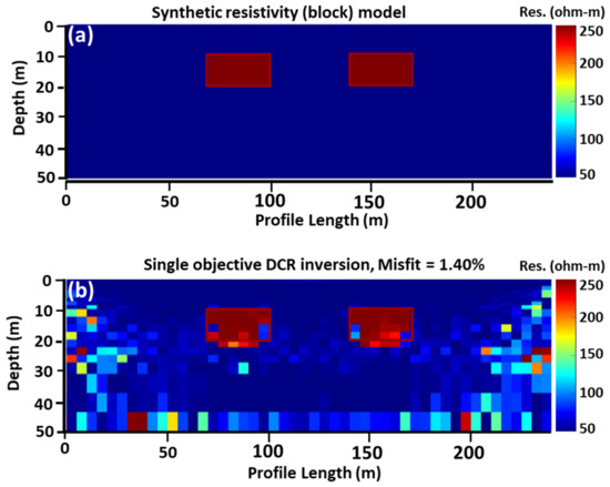
Figure 12.
Positive anomaly model inversion using the single objective global optimization method; (a) synthetic dc-resistivity model and (b) single object inverted resistivity model. The dark red line is used to mark the anomaly boundary.
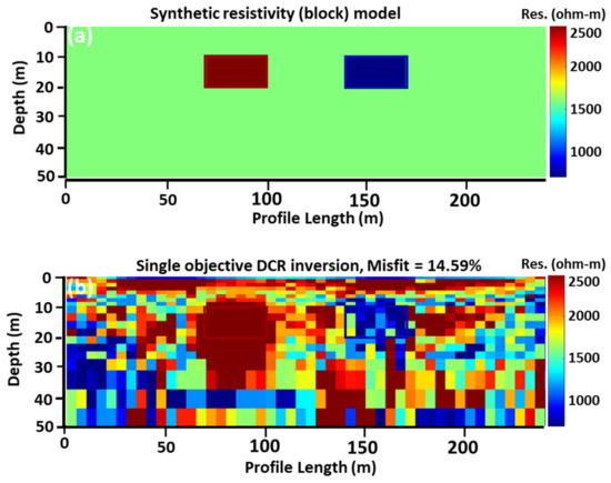
Figure 13.
Positive and negative anomaly model inversion using the single objective global optimization method; (a) synthetic dc-resistivity model and (b) single object inverted resistivity model. The dark red/blue lines are used to mark the anomaly boundary.
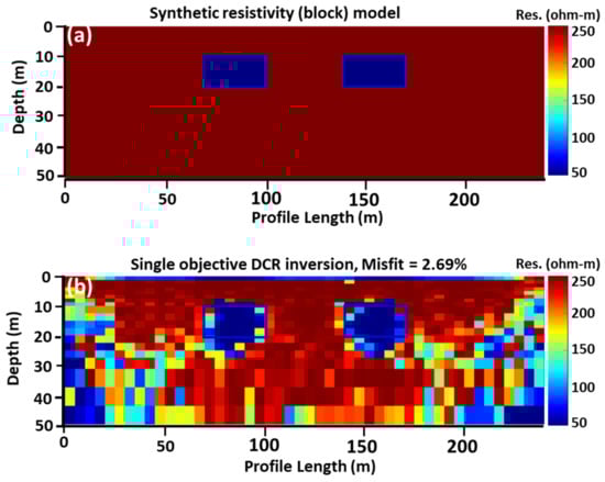
Figure 14.
Negative anomaly model inversion using the single objective global optimization method; (a) synthetic dc-resistivity model and (b) single object inverted resistivity model. The dark blue line is used to mark the anomaly boundary.
4. Discussion
The local optimization algorithm performed optimally in delineating both resistivity and velocity anomalies regarding the tested models. This result is attributed to the application of the smoothing term and appropriate regularization parameters in the objective function to mitigate the effect of the non-uniqueness of the inverse problem. Table 2, Table 3 and Table 4 summarize the performance of both LOM and CGO algorithms in the inversion involving both DCR and SR methods. Generally, the results from Table 2, Table 3 and Table 4 show that the CGO improved the misfits compared with the LOM in both the DCR and SR methods but at a relatively high computation cost. Table 5 summarizes the results of the CGO for both (DCR and SR) synthetic models. Despite using a parallel computing approach, the GOM results showed a run time of 6642.15 to 13,962.00 min. This suggests that the most significant challenge with applying the GOM algorithm is the run time.
Table 2.
Local and global optimization inversion results parameter for both DCR and SR (synthetic dyke anomaly model) methods.
Table 3.
Local and combined (local plus global) optimization inversion results parameters for both DCR and SR (synthetic positive anomaly model) methods.
Table 4.
Local and global optimization inversion results parameters for both DCR and SR (synthetic positive and negative anomalies model) methods.
Table 5.
Summary of the convectional global optimization inversion results parameter for both DCR and SR (dyke, positive, positive and negative anomalies model) methods.
The results showed that the CGO algorithm inherited some features of the model, such as the geometry and amplitude of the anomaly from the local optimization that reflects in its optimum performance. For example, the amplitude and geometry of the DCR in the Dyke model was reflected in the final output of global optimization (Figure 6). Notice that in Figure 9d and Figure 10d, the ray path avoided the negative anomaly; thus, the ideal model structure cannot be reconstructed with high resolution. This scenario is peculiar with the application of the SR method regarding a low-velocity layer (e.g., cavity) surrounded by a high-velocity media [48].
In the CGO method, using the same size of the synthetic model from the LOM, we observed that obtaining a good inversion result for the SR model using a computer with 12 logical processors configuration (6 cores) takes a longer time than the DCR method. This is because the DCR method produces electrical perturbation and estimates the apparent resistivity of the model at once; however, the SR method first computes the travel time from one source to all receivers sequentially and thereafter repeats the same procedure for all other available sources. To optimize the computation time of both SOO and MOO, we made the misfit algorithm part of the code to run on parallel computing by using the built-in parallel computing (e.g., parfor loop) command in MATLAB. This process enhanced the computation cost of the hybrid global optimization algorithm. For instance, it took 189.75 min to obtain the same result as in Figure 8b (single-objective GA for the positive anomaly DCR model) without parallel computing, whereas it took 55.25 min (71% run time optimization) to obtain the same output with parallel computing. Similarly, running the single objective genetic algorithm for the positive anomaly velocity (SR) model for 100 generations took 664.56 min without parallel computing, whereas it took 75.66 min (89% run time optimization) to obtain the same result with parallel computing. The percentage of run time optimization depends on the population size, number of generations, and type of geophysical method involved. To make the synthetic test challenging for the CGO algorithm, we added 3% Gaussian noise to the data resulting from the positive anomaly model. Although the output did not match noise-free data perfectly, a larger portion of the anomaly was recovered (Figure 15 and Figure 16).
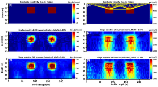
Figure 15.
Test of the combined optimization algorithm using data (both DCR and SR) with added 3% gaussian noise; (a) synthetic dc-resistivity model, (b) single objective inverted resistivity model (noisy), (c) single objective inverted resistivity model (noiseless), (d) synthetic velocity model, (e) single objective inverted velocity model (noisy), and (f) single objective inverted velocity model (noiseless). The dark red lines are used to mark the anomaly boundary.
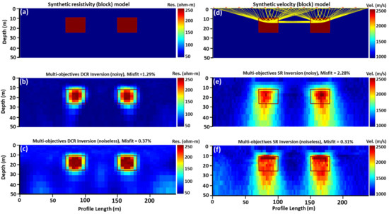
Figure 16.
Test of the combined optimization algorithm using data (both DCR and SR) with added 3% gaussian noise; (a) synthetic dc-resistivity model, (b) multi-objectives inverted resistivity model (noisy), (c) multi-objectives inverted resistivity model (noiseless), (d) synthetic velocity model, (e) multi-objectives inverted velocity model (noisy), and (f) multi-objectives inverted velocity model (noiseless). The dark red lines are used to mark the anomaly boundary.
Regarding the GA population size, we observed that the CGO algorithm involving the DCR and SR methods performed better with an increasing number of populations. For example, Figure 15 shows a graduate improvement in the model resolution as the number of populations increased in the DCR genetic algorithm result. Similarly, the CGO algorithm offered a better performance with increasing generations. Notwithstanding, increasing the number of populations and generations prolonged the computation run time (Figure 17).
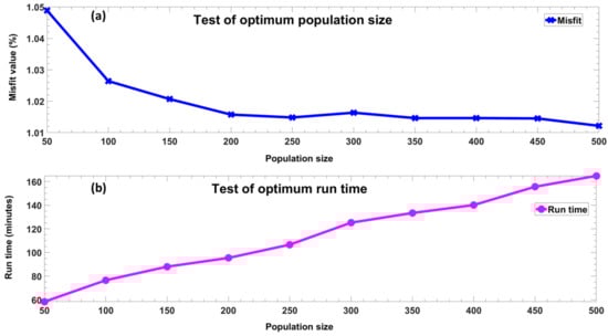
Figure 17.
Effect of population size on DC-resistivity inversion using the genetic algorithm; (a) test of optimum population size that produces the most significant misfit and (b) test of optimum run time with respect to population size.
Considering these criteria (number of generations, population size, and computation time), we applied an average population size of 500 and 500 generations for both DCR and SR combined global optimization inversions.
5. Conclusions
The proposed CGO used in this study begins with the application of a local optimization algorithm that requires the use of appropriate regularization parameters incorporated into the DCR and SR objective functions, and it is optimized (using the LOM) to obtain the best model, which will be used as an input model for the combined local–global optimization CGO method. This study applied this concept to obtain the best model parameters for both an individual and joint inversion of the DCR and SR geophysical methods. The CGO algorithm used to overcome the challenges associated with the separate application of LOM and GOM involved the application of the final output (optimum model parameter) of the LOM as the input for the CGO techniques. The global optimization part of the single objective CGO applied the GA to optimize the DCR and SR misfit functions (Equations (13) and (14), respectively) while the NSGA II was used to optimize the resultant misfit from the DCR and SR in the multi-objective optimization algorithm. Apart from the CGO method, which improved the computation run time, we made a part (the misfit function) of the CGO algorithm run on parallel computing. This approach not only contributed to the optimization of the CGO algorithm run time but also provided an opportunity to test the convectional GOM using a computer with 12 logical processor units (six cores). The CGO algorithm was tested with both resistivity and velocity models that had a dyke, two blocks (positive), and two blocks (positive and negative) anomalies. Generally, the CGO algorithm showed an improvement when compared with the local optimization output (Table 2, Table 3 and Table 4). However, the conventional GOM results showed instability in the delineation of the anomalies in all the tested SR and DCR models, and the model instability was probably due to the use of an unconstraint objective function. However, the CGO method overcame the challenge of model instability since it was linearly constrained by using the LOM’s output to define the search space’s lower and upper bounds. Additionally, the conventional GOM application remained computationally expensive (especially for the SR method) relative to the CGO techniques. Therefore, this study recommends applying a combined approach (local and global optimization algorithm) when characterizing the subsurface when both DCR and SR data are acquired.
Author Contributions
Conceptualization, P.S.; methodology, I.D., I.A., H.A.H., P.S., and E.C.; software, P.E., I.D., I.A., and H.A.H.; validation, I.D., I.A., and H.A.H.; formal analysis, P.E., I.D., I.A., H.A.H., P.S., and E.C.; resources, P.S.; data curation, P.E., I.D., I.A., H.A.H., P.K., and P.S.; writing—original draft preparation, P.E., I.D., I.A., H.A.H., P.K., and P.S.; writing—review and editing, P.E., I.D., I.A., H.A.H., P.K., P.S., E.C., S.H., and A.A.-S.; visualization, P.E., P.K., and P.S.; supervision, P.S.; project administration, P.S.; funding acquisition, A.A.-S. All authors have read and agreed to the published version of the manuscript.
Funding
This research was funded by the start-up grant SF18060 from the College of Petroleum Engineering and Geosciences (CPG) at King Fahd University of Petroleum and Minerals (KFUPM).
Institutional Review Board Statement
Not applicable.
Informed Consent Statement
Not applicable.
Data Availability Statement
Not applicable.
Conflicts of Interest
The authors declare no conflict of interest. The funders had no role in the design of the study; in the collection, analyses, or interpretation of data; in the writing of the manuscript; or in the decision to publish the results.
References
- Oldenburg, D.W.; Ellis, R.G. Inversion of geophysical data using an approximate inverse mapping. Geophys. J. Int. 1991, 105, 325–353. [Google Scholar] [CrossRef]
- Oldenburg, D.W.; Li, Y. Inversion for Applied Geophysics: A Tutorial. In Near-Surface Geophysics; Society of Exploration Geophysicists: Houston, TX, USA, 2005; pp. 89–150. [Google Scholar]
- Farquharson, C.G.; Oldenburg, D.W. A comparison of automatic techniques for estimating the regularization parameter in non-linear inverse problems. Geophys. J. Int. 2004, 156, 411–425. [Google Scholar] [CrossRef]
- Fomel, S. Shaping regularization in geophysical-estimation problems. Geophysics 2007, 72, R29. [Google Scholar] [CrossRef]
- Gheymasi, H.M.; Gholami, A. A local-order regularization for geophysical inverse problems. Geophys. J. Int. 2013, 195, 1288–1299. [Google Scholar] [CrossRef]
- Gündoğdu, N.Y.; Demirci, İ.; Demirel, C.; Candansayar, M.E. Characterization of the bridge pillar foundations using 3d focusing inversion of DC resistivity data. J. Appl. Geophys. 2020, 172, 103875. [Google Scholar] [CrossRef]
- Haber, E.; Oldenburg, D. Joint inversion: A structural approach. Inverse Probl. 1997, 13, 63–77. [Google Scholar] [CrossRef]
- Gallardo, L.A.; Meju, M.A. Characterization of heterogeneous near-surface materials by joint 2D inversion of dc resistivity and seismic data. Geophys. Res. Lett. 2003, 30, 1658. [Google Scholar] [CrossRef]
- Gallardo, L.A.; Meju, M.A. Joint two-dimensional cross-gradient imaging of magnetotelluric and seismic traveltime data for structural and lithological classification. Geophys. J. Int. 2007, 169, 1261–1272. [Google Scholar] [CrossRef]
- Linde, N.; Binley, A.; Tryggvason, A.; Pedersen, L.B.; Revil, A. Improved hydrogeophysical characterization using joint inversion of cross-hole electrical resistance and ground-penetrating radar traveltime data. Water Resour. Res. 2006, 42, W12404. [Google Scholar] [CrossRef]
- Infante, V.; Gallardo, L.A.; Montalvo-Arrieta, J.C.; Navarro de León, I. Lithological classification assisted by the joint inversion of electrical and seismic data at a control site in northeast Mexico. J. Appl. Geophys. 2010, 70, 93–102. [Google Scholar] [CrossRef]
- Moorkamp, M.; Heincke, B.; Jegen, M.; Roberts, A.W.; Hobbs, R.W. A framework for 3-D joint inversion of MT, gravity and seismic refraction data. Geophys. J. Int. 2011, 184, 477–493. [Google Scholar] [CrossRef]
- Hamdan, H.A.; Vafidis, A. Joint inversion of 2D resistivity and seismic travel time data to image saltwater intrusion over karstic areas. Environ. Earth Sci. 2013, 68, 1877–1885. [Google Scholar] [CrossRef]
- Bennington, N.L.; Zhang, H.; Thurber, C.H.; Bedrosian, P.A. Joint Inversion of Seismic and Magnetotelluric Data in the Parkfield Region of California Using the Normalized Cross-Gradient Constraint. Pure Appl. Geophys. 2015, 172, 1033–1052. [Google Scholar] [CrossRef]
- Demirci, İ.; Candansayar, M.E.; Vafidis, A.; Soupios, P. Two dimensional joint inversion of direct current resistivity, radio-magnetotelluric and seismic refraction data: An application from Bafra Plain, Turkey. J. Appl. Geophys. 2017, 139, 316–330. [Google Scholar] [CrossRef]
- Demirci, İ.; Dikmen, Ü.; Candansayar, M.E. Two-dimensional joint inversion of Magnetotelluric and local earthquake data: Discussion on the contribution to the solution of deep subsurface structures. Phys. Earth Planet. Inter. 2018, 275, 56–68. [Google Scholar] [CrossRef]
- Wang, K.P.; Tan, H.D.; Wang, T. 2D joint inversion of CSAMT and magnetic data based on cross-gradient theory. Appl. Geophys. 2017, 14, 279–290. [Google Scholar] [CrossRef]
- Vozoff, K.; Jupp, D.L.B. Joint Inversion of Geophysical Data. Geophys. J. Int. 1975, 42, 977–991. [Google Scholar] [CrossRef]
- Autio, U.; Smirnov, M.Y.; Savvaidis, A.; Soupios, P.; Bastani, M. Combining electromagnetic measurements in the Mygdonian sedimentary basin, Greece. J. Appl. Geophys. 2016, 135, 261–269. [Google Scholar] [CrossRef]
- Demirci, İ.; Gündoğdu, N.Y.; Candansayar, M.E.; Soupios, P.; Vafidis, A.; Arslan, H. Determination and Evaluation of Saltwater Intrusion on Bafra Plain: Joint Interpretation of Geophysical, Hydrogeological and Hydrochemical Data. Pure Appl. Geophys. 2020, 177, 5621–5640. [Google Scholar] [CrossRef]
- Vafidis, A.; Soupios, P.; Economou, N.; Hamdan, H.; Andronikidis, N.; Kritikakis, G.; Panagopoulos, G.; Manoutsoglou, E.; Steiakakis, M.; Candansayar, E.; et al. Seawater intrusion imaging at Tybaki, Crete, using geophysical data and joint inversion of electrical and seismic data. First Break 2014, 32, 107–114. [Google Scholar] [CrossRef]
- Shahrukh, M.; Soupios, P.; Papadopoulos, N.; Sarris, A. Geophysical investigations at the Istron archaeological site, eastern Crete, Greece using seismic refraction and electrical resistivity tomography. J. Geophys. Eng. 2012, 9, 749–760. [Google Scholar] [CrossRef]
- Linde, N.; Doetsch, J. Joint Inversion in Hydrogeophysics and Near-Surface Geophysics. In Integrated Imaging of the Earth: Theory and Applications; John Wiley & Sons: Hoboken, NJ, USA, 2016; pp. 117–135. [Google Scholar]
- Meju, M.A. Joint multi-geophysical inversion: Effective model integration, challenges and directions for future research. In Proceedings of the International Workshop on Gravity, Electrical & Magnetic Methods and Their Applications, Beijing, China, 10–13 October 2011; p. 37. [Google Scholar] [CrossRef]
- Athanasiou, E.N.; Tsourlos, P.I.; Papazachos, C.B.; Tsokas, G.N. Combined weighted inversion of electrical resistivity data arising from different array types. J. Appl. Geophys. 2007, 62, 124–140. [Google Scholar] [CrossRef]
- Hu, W.; Abubakar, A.; Habashy, T.M. Joint electromagnetic and seismic inversion using structural constraints. Geophysics 2009, 74, R99–R109. [Google Scholar] [CrossRef]
- Bastani, M.; Hübert, J.; Kalscheuer, T.; Pedersen, L.B.; Godio, A.; Bernard, J. 2D joint inversion of RMT and ERT data versus individual 3D inversion of full tensor RMT data: An example from Trecate site in Italy. Geophysics 2012, 77, WB233–WB243. [Google Scholar] [CrossRef]
- Gallardo, L.A.; Fontes, S.L.; Meju, M.A.; Buonora, M.P.; De Lugao, P.P. Robust geophysical integration through structure-coupled joint inversion and multispectral fusion of seismic reflection, magnetotelluric, magnetic, and gravity images: Example from Santos Basin, offshore Brazil. Geophysics 2012, 77, B237–B251. [Google Scholar] [CrossRef]
- Lochbühler, T.; Doetsch, J.; Brauchler, R.; Linde, N. Structure-coupled joint inversion of geophysical and hydrological data. Geophysics 2013, 78, ID1–ID14. [Google Scholar] [CrossRef]
- Zhang, Y.; Zhao, Z.; Nie, Z.; Liu, Q.H. Approach on Joint Inversion of Electromagnetic and Acoustic Data Based on Structural Constraints. IEEE Trans. Geosci. Remote Sens. 2020, 58, 7672–7681. [Google Scholar] [CrossRef]
- Yin, C.; Sun, S.; Liu, Y.; Ren, X.; Wang, C. Joint inversion of geophysical data and applications. In Proceedings of the Fifth International Conference on Engineering Geophysics, Al Ain, United Arab Emirates, 21–24 October 2019; pp. 232–235. [Google Scholar] [CrossRef]
- Jordi, C.; Doetsch, J.; Günther, T.; Schmelzbach, C.; Maurer, H.; Robertsson, J.O.A. Structural joint inversion on irregular meshes. Geophys. J. Int. 2020, 220, 1995–2008. [Google Scholar] [CrossRef]
- Liu, S.; Liang, M.; Hu, X. Particle swarm optimization inversion of magnetic data: Field examples from iron ore deposits in China. Geophysics 2018, 83, J43–J59. [Google Scholar] [CrossRef]
- Rani, P.; Piegari, E.; Di Maio, R.; Vitagliano, E.; Soupios, P.; Milano, L. Monitoring time evolution of self-potential anomaly sources by a new global optimization approach. Application to organic contaminant transport. J. Hydrol. 2019, 575, 955–964. [Google Scholar] [CrossRef]
- Soupios, P.; Akca, I.; Mpogiatzis, P.; Basokur, A.T.; Papazachos, C. Applications of hybrid genetic algorithms in seismic tomography. J. Appl. Geophys. 2011, 75, 479–489. [Google Scholar] [CrossRef]
- Akça, I.; Basokur, A.T. Extraction of structure-based geoelectric models by hybrid genetic algorithms. Geophysics 2010, 75, F15–F22. [Google Scholar] [CrossRef]
- Chunduru, R.K.; Sen, M.K.; Stoffa, P.L. Hybrid optimization methods for geophysical inversion. Geophysics 2012, 62, 1196–1207. [Google Scholar] [CrossRef]
- Schwarzbach, C.; Börner, R.-U.; Spitzer, K. Two-dimensional inversion of direct current resistivity data using a parallel, multi-objective genetic algorithm. Geophys. J. Int. 2005, 162, 685–695. [Google Scholar] [CrossRef]
- Ayani, M.; MacGregor, L.; Mallick, S. Inversion of marine controlled source electromagnetic data using a parallel non-dominated sorting genetic algorithm. Geophys. J. Int. 2020, 220, 1066–1077. [Google Scholar] [CrossRef]
- Akca, İ.; Günther, T.; Müller-Petke, M.; Başokur, A.T.; Yaramanci, U. Joint parameter estimation from magnetic resonance and vertical electric soundings using a multi-objective genetic algorithm. Geophys. Prospect. 2014, 62, 364–376. [Google Scholar] [CrossRef]
- Holland, J.H. Adaptation in Natural and Artificial Sytems; An Introductory Analysis with Applications to Biology, Control, and Artificial Intelligence; Bradford Book: Denver, CO, USA, 1992; ISBN 978-0262581110. [Google Scholar]
- Goldberg, D.E. Genetic Algorithms in Search, Optimization and Machine Learning; Addison-Wesley Longman Publishing Co., Inc.: Boston, MA, USA, 1989; Volume 7, ISBN 0201157675. [Google Scholar]
- Sen, M.K.; Stoffa, P.L. Global Optimization Methods in Geophysical Inversion; Cambridge University Press: Cambridge, UK, 2013; ISBN 1139619519. [Google Scholar]
- Zidan, A.; Li, Y.E.; Cheng, A. A Pareto Multi-Objective Optimization Approach for Anisotropic Shale Models. J. Geophys. Res. Solid Earth 2021, 126, e2020JB021476. [Google Scholar] [CrossRef]
- Deb, K.; Pratap, A.; Agarwal, S.; Meyarivan, T. A fast and elitist multiobjective genetic algorithm: NSGA-II. IEEE Trans. Evol. Comput. 2002, 6, 182–197. [Google Scholar] [CrossRef]
- Soupios, P.; Papazachos, C.B.; Vallianatos, F.; Papakostas, T. Numerical treatment and evaluation of inverse problems. WSEAS Trans. Circuits Syst. 2003, 2, 547–551. [Google Scholar]
- Soupios, P.M.; Papazachos, C.B.; Juhlin, C.; Tsokas, G.N. Nonlinear 3-D traveltime inversion of crosshole data with an application in the area of the Middle Ural mountains. Geophysics 2001, 66, 627–636. [Google Scholar] [CrossRef]
- Carollo, A.; Capizzi, P.; Martorana, R. Joint interpretation of seismic refraction tomography and electrical resistivity tomography by cluster analysis to detect buried cavities. J. Appl. Geophys. 2020, 178, 104069. [Google Scholar] [CrossRef]
Publisher’s Note: MDPI stays neutral with regard to jurisdictional claims in published maps and institutional affiliations. |
© 2022 by the authors. Licensee MDPI, Basel, Switzerland. This article is an open access article distributed under the terms and conditions of the Creative Commons Attribution (CC BY) license (https://creativecommons.org/licenses/by/4.0/).