Im2mesh: A Python Library to Reconstruct 3D Meshes from Scattered Data and 2D Segmentations, Application to Patient-Specific Neuroblastoma Tumour Image Sequences

Abstract

The future of personalised medicine lies in the development of increasingly sophisticated digital twins, where the patient-specific data is fed into predictive computational models that support the decisions of clinicians on the best therapies or course actions to treat the patient’s afflictions. The development of these personalised models from image data requires a segmentation of the geometry of interest, an estimation of intermediate or missing slices, a reconstruction of the surface and generation of a volumetric mesh and the mapping of the relevant data into the reconstructed three-dimensional volume. There exist a wide number of tools, including both classical and artificial intelligence methodologies, that help to overcome the difficulties in each stage, usually relying on the combination of different software in a multistep process. In this work, we develop an all-in-one approach wrapped in a Python library called im2mesh that automatizes the whole workflow, which starts reading a clinical image and ends generating a 3D finite element mesh with the interpolated patient data. In this work, we apply this workflow to an example of a patient-specific neuroblastoma tumour. The main advantages of our tool are its straightforward use and its easy integration into broader pipelines.

1. Introduction

Personalised medicine [1] is based on the idea that inter-individual variability conditions define how a certain disease affects each person and that specific actions can be tailored to the patients based on their predicted response or risks. In recent years, there has been a continuous growth in this field thanks in part to the improvements on medical imaging techniques, genetic data acquisition and clinical tools for disease diagnosis and prognosis [2,3,4].

In parallel, there has also been a notable development in in silico medicine, also known as “computational medicine”, due to the huge technical advances and the availability of improved software and hardware that allows the simulation of increasingly complex and demanding problems. In the biomedical field, these simulations aim to provide additional information that helps to understand the intricacies of biological processes, which may be useful to develop tools to support clinical decisions [5]. Given the importance of personalised medicine, in particular for the treatment of cancer, researchers keep developing new in silico tools that account for individualised data, a field of expertise known as patient-specific modelling. These models simulate biological processes, often related to disease, using particular data from the patient. This combination of mathematical models and individualized parameters holds the key to a future, where digital twins might be used to improve the diagnosis and select the best possible treatment for a specific condition [6,7,8].

Despite the aforementioned advances made in its diagnosis and treatment, cancer is still the second most common cause of death in the world, being responsible for about one-sixth of total deaths [9]. It is a very complex and heterogeneous disease due to the great number of biological and mechanical factors that control tumour growth, treatment efficacy and metastasis, among other processes. Differences arise not only between different types of cancer, but also among individuals afflicted by the same type.

Within this context of heterogeneity, patient-specific models constitute a great option to support decision making in the clinical management of the disease. There are several examples of tumour growth models that incorporate personalised data, often derived from imaging sequences, which can be magnetic resonance imaging (MRI), computed tomography (CT), etc. [10,11,12]. Examples of these sequences include diffusion-weighted imaging (DWI) and dynamic contrast enhanced (DCE) in the case of MRI or dual energy computed tomography (DECT) for CT. They can be used to obtain insightful knowledge of the cellularity level (DWI) and vascularization (DCE and DECT) of the tissue, which are the main inputs for most of these tumour growth models.

To include this imaging data in a model, the first step is to incorporate the geometry of the tumour and, if available, of surrounding organs. Therefore, one should start by segmenting the region of interest (ROI) in one of the imaging series and then registering the other sequences to this segmented series, which is critical to have all imaging data (geometry, cellularity and vascularization data) in the same coordinate system. Regarding the segmentation task, there are several ways to segment the different tissues [13]. The first and most traditional way is manual or partially-assisted segmentation, where a professional (a radiologist in clinical practice) delineates the ROIs and generates the masks in every individual slice. Although very accurate, the process is time-consuming and often infeasible when the number of cases is too large, which often leads to partial segmentations, where particular slices are skipped (i.e., when the object of interest presents no abrupt changes with respect to the previous segmented slice and the mask would be almost identical). This can be alleviated to some extent via semi-automatic segmentation, which applies statistical and machine learning methods to propose masks that need to be revised and manually corrected by an experienced professional [14,15]. In recent years, the boom of artificial intelligence for image applications has laid the foundation for the development of algorithms that apply the power of deep learning to automate the task of segmentation with very promising results [16].

Regardless of the segmentation method used, the next step is reconstructing the original 3D geometry from the stack of segmented slices. This volume generation might be included in the own architecture of the DL network (such as U-Net [17]). Otherwise, a subsequent step of 3D reconstruction is needed. There is a wide range of methods to perform volume generation from a set of 2D slices [18,19], some of them already included as features of popular software such as 3D Slicer [20]. This process of segmentation and volume reconstruction culminates with the interpolation of the different image sequence data to the generated volumetric mesh. These interpolated maps together with the geometry constitute the necessary inputs for the construction of the patient-specific models previously described.

To illustrate this methodology, we present a practical use case within the PRIMAGE project (PRedictive In -silico Multiscale Analytics to support cancer personalised diaGnosis and prognosis, Empowered by imaging biomarkers) [21,22], where the described workflow was used to generate patient-specific models in a large number of clinical cases. To put it into context, PRIMAGE is currently one of the largest and more ambitious European research projects in medical imaging, artificial intelligence and childhood cancer, in particular, neuroblastoma (NB) and diffuse intrinsic pontine glioma (DIPG). Its main goal is to develop a decision support system combining retrospective clinical information and incorporating it into the diagnostic pipeline using AI and computational models. One of the peculiarities of this project is the availability of tumour segmentations from hundreds of patients, which need to be processed and incorporated into an automatized workflow to simulate the tumour progression with patient-specific data. This decision support system will be integrated in an online platform and used by clinicians in their day-to-day practice, hence the necessity of self-contained tools (i.e., no extra software or technical parameter handling needed) that can be used via regular browsers. With this idea in mind, we developed im2mesh, which has no particular requirements other than an environment supporting Python 3.9 and can be executed both in bash mode (therefore integrated for example into an automatized cloud-based platform) and with a minimal user interface when used for research purposes. We would like to emphasize that im2mesh aims to be a tool for a very specific task: transforming segmented slices into 3D meshes (with or without interpolated data) that can be used as a connecting component between image data and simulations. Certainly, there are other well-established tools, such as 3D Slicer (open software) or Mimics (Materialise, Leuven, Belgium), with big communities and a wide range of functionalities and versatility, but which are designed to be used as visual user-interactive tools rather than “black box” functions for automatization.

In this work, we describe in detail the proposed methodology. Then, we compare our 3D reconstruction with that obtained with 3D Slicer, we analyse mesh quality, and we study the effect of downsampling (decreased number of slices) on geometry details. Finally, we analyse a clinical example taken from the PRIMAGE platform, corresponding to a neuroblastoma tumour.

2. Materials and Methods

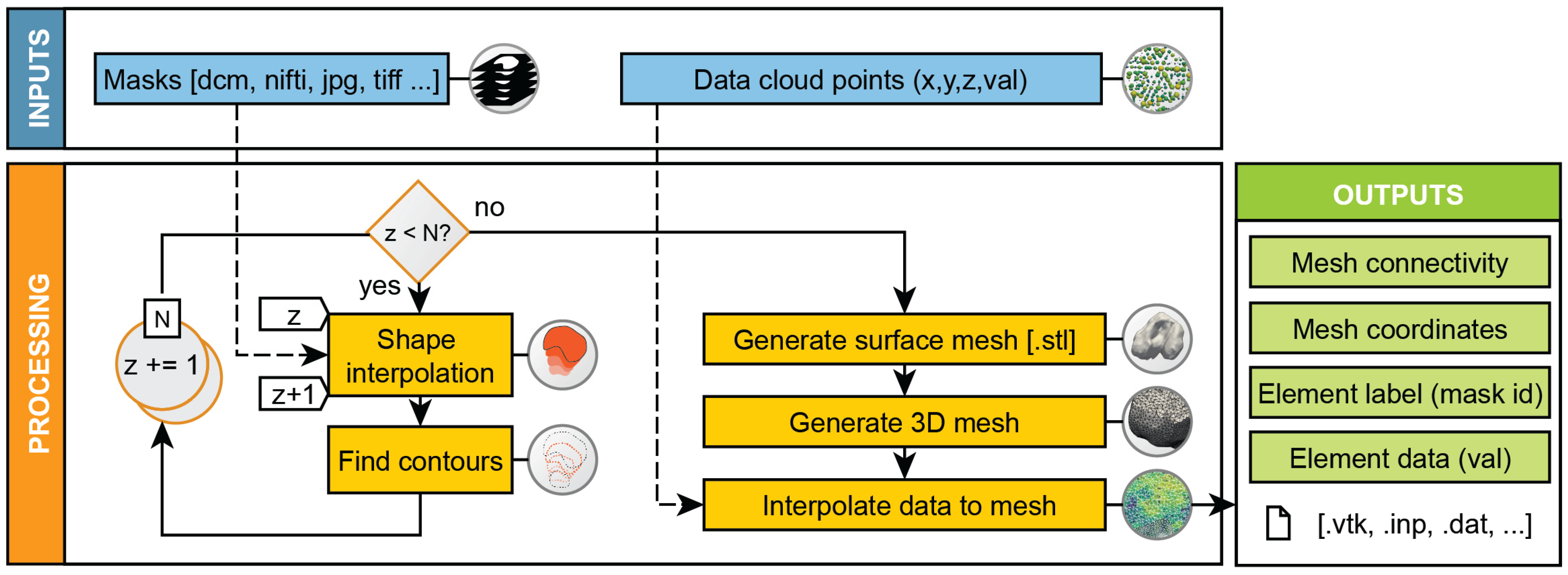
In this section, we provide a summary of the developed workflow, describing in detail the algorithms and methods used for surface and volume generation. Finally, we provide the sources for the code, its documentation and the data presented in this work.

2.1. Workflow

Our library accepts multiple image formats and input parameters that are prompted to the user either via command (bash-mode) or via visual interfaces. In particular, typical medical image formats such as NIfTI (.nii), DICOM and DICOM-SEG (.dcm), as well as regular image formats supported by OpenCV [23] can be used. The input stack, composed of any number (N) of slices or layers (previously segmented), is processed from bottom to top, interpolating shapes between every pair of layers. The contours of the original layers, plus the interpolated (virtual) ones, are stored for the surface mesh generation. Note that the inside points of the top and bottom layers of the whole stack are also included to obtain a closed surface, which is used later to obtain a 3D tetrahedral mesh. Optionally, a cloud of values (position coordinates plus scalar value) can be extracted from the medical files or provided by the user to be interpolated to the elements of this mesh. We include a last step that allows exporting the generated mesh to different formats appropriate for commercial Finite Element software commonly used in engineering such as ABAQUS (Dassault Systèmes, Paris, France) or ANSYS (Ansys, Inc., Pittsburgh, PA, USA). A schematic representation of the workflow is shown in Figure 1.

2.2. Shape Interpolation

Shape interpolation is performed by following the steps illustrated in the benchmark example shown in Figure 2, using the methodology described in [24]. The necessary inputs to interpolate between two layers are just the binarized representations (BW) of each layer. Firstly, the contour or perimeter of each layer is computed (BW_per), and the signed Euclidean distance (S_edist) between each pixel and the perimeter is calculated. This distance is equivalent to the regular Euclidean distance but considered negative for pixels outside the perimeter and positive for those inside (Figure 2A).

Once the signed distances are computed for both layers, their values are linearly interpolated to any number of intermediate layers (Figure 2B left). The new layers are converted back to a binary image by thresholding negative values (Figure 2B right).

This procedure is repeated between every pair of consecutive layers until the whole stack has been processed (Figure 2C). Finally, the contours of each of the binary layers are extracted using the OpenCV library [23] and their coordinates stored to form the superficial point cloud.

2.3. Mesh Generation

Surface meshes (Figure 2D left) are generated via the Python library PyMeshLab that in turn interfaces with the popular open-source application MeshLab [25], using as input a cloud of 3D points coming from the contours computed by the shape interpolation algorithm. To enhance the robustness of the algorithm (e.g., avoiding over-sensitivity of convergence due to a wrong ratio of the number of pixels per layer and number of intermediate interpolations), the cloud points are randomly sampled following the Poisson Disk sampling method [26], ensuring homogeneous spatial distribution. This algorithm takes as inputs an estimation of the number of points sampled, which is defined as a fraction of the number of points in the original cloud.

Then, the algorithm computes the normals for the sampled point cloud and finally generates a closed surface based on these normals using the Screened Poisson surface reconstruction method [27]. To improve the quality of the volumetric mesh to be generated afterwards, a decimating filter is added after the surface reconstruction. This filter is based on the quadric based edge-collapsed strategy [28]. Additionally, the generated surface can be smoothed (user-defined option) to simplify complex geometries that could be problematic for the subsequent volumetric meshing. We employ the HC Laplacian Smoothing [29] algorithm for this purpose.

Figure 2. A whole-process demonstration example with an input of three binary layers representing the X, Y and Z letters: (A) signed Euclidean distance map of the first two masks (X and Y shapes). Pixels inside the perimeter (red line) present positive distances, whereas exterior pixels are assigned negative values; (B) distance maps are interpolated in any number of intermediate layers (left vertical cut) and thresholded to return a binarized volume (1 if distance > 0; 0 otherwise); (C) interpolation of 10 intermediate positions (equally distributed) between input and output layers; (D) surface mesh reconstruction (.stl format) (left panel), and 3D tetrahedral mesh generated with a transversal cut (middle panel). Insets 1 and 2 show the smoothness and good quality of the elements (right panel).

Figure 2. A whole-process demonstration example with an input of three binary layers representing the X, Y and Z letters: (A) signed Euclidean distance map of the first two masks (X and Y shapes). Pixels inside the perimeter (red line) present positive distances, whereas exterior pixels are assigned negative values; (B) distance maps are interpolated in any number of intermediate layers (left vertical cut) and thresholded to return a binarized volume (1 if distance > 0; 0 otherwise); (C) interpolation of 10 intermediate positions (equally distributed) between input and output layers; (D) surface mesh reconstruction (.stl format) (left panel), and 3D tetrahedral mesh generated with a transversal cut (middle panel). Insets 1 and 2 show the smoothness and good quality of the elements (right panel).

Three-dimensional meshes (Figure 2D middle) are then generated from the surface files (.stl) using the open-source library Gmsh [30] which provides great flexibility.

2.4. Evaluation Metrics

To prove the robustness and accuracy of our algorithm with respect to other well-established software [20], we compare the surface meshes generated. The metric used for this comparison is the Intersection over Union (IoU), defined as:

$$IoU=\left(A\cap B\right) / \left(A\cup B\right)$$

where p<a and B are two different volumes enclosed by the generated surface meshes. The IoU is 1 when both objects are equal and overlap totally. It should be noted that, unlike in the computer vision field, the registration step can be skipped since our volumes are aligned in the 3 spatial axes, which simplifies the computation of the IoU considerably.

We also perform an analysis of the quality of the volumetric mesh obtained from Gmsh. For this purpose, we have chosen two arbitrary metrics: the Aspect Ratio (AR) and the Aspect Frobenius (AF) [31], which compute how far the analysed mesh is from an ideal mesh. The AR is defined as the ratio of the maximum edge with respect to the radius of the element’s inscribed sphere:

$$AR=max\left(x_1,x_2,\dots ,x_6\right)/2\ast \sqrt{6}\ast r$$

where $x_1$ to $x_6$ are the length of the edges in a tetrahedron, and $r$ is the radius of the sphere inscribed in the tetrahedral element.

The AF of an element is the normalised Frobenius condition number of matrix $A_0$. The mathematical expression for the Frobenius condition number of an element is:

$${\left|A_0\right|}_F=\sqrt{tr\left(A_0{}^T{A}_0\right)}$$

(1)

where $A_0=T_0{W}^{-1}$. $T_0$ is the edge matrix of the tetrahedral element, and $W$ is the edge matrix of the reference regular tetrahedron.

Both metrics are normalised, i.e., they equal one when the element analysed is the ideal regular element. According to other authors [31], acceptable ranges are [1, 3] and [1, 1.3] for the AR and AF, respectively.

2.5. Data Interpolation

Once the FE mesh is generated, the additional imaging data that may be available must be interpolated to this mesh. Most patient-specific models, especially tumour growth models, need as inputs not only the geometry, but also other spatial distributions of properties that describe the heterogeneous characteristics of tumours. In the case of PRIMAGE, this additional data was obtained from DWI and DCE sequences, respectively. These MRI sequences are commonly used in clinical practice to evaluate the cellularity and vascularization of the tumours. The cellularity values are derived from the Apparent Diffusion Coefficient maps generated from DWI sequences [32], while the vascularization is obtained from the analysis of DCE sequences [33]. Apart from these sequences, there are many other techniques to obtain different imaging data that might be included in the FE mesh. Therefore, our code includes a script to read any kind of data derived from imaging that is stored in NIfTI and DICOM formats and interpolate it to any FE mesh given. The interpolation process begins by transforming the imaging data to be interpolated from voxel coordinates to global coordinates using the affine matrix of each imaging sequence. Then, we use the Scipy [34] Python library to interpolate the spatial data to the elemental centroids of the mesh generated previously, exporting this interpolated data to an additional file that can be used as input for subsequent computational models.

3. Results

This section is divided into three different parts. In the first we compare our library to 3D Slicer software by reconstructing a human pelvis using both methods and measuring the differences. The next part covers the effects of reducing the number of available slices in the segmentation (what we define as downsampling) using the same example. Finally, we show the application of the workflow summarised in Figure 1 on one of the NB cases available in the PRIMAGE project dataset.

3.1. Volume Reconstruction

In this section, we make use of our library to reconstruct a pelvis (plus part of the femurs) from a partial segmentation obtained from the Cancer Imaging Archive public repository and compare it to that obtained using the software 3D Slicer. Figure 3 shows the surface volume reconstructed after processing a 512 × 512 × 300 volumetric image both with im2mesh (Figure 3A orange, left) and 3D Slicer (Figure 3A blue, right). Visual differences between both surfaces are minimal (Figure 3B), as confirmed by an IoU score of 98.6%. Note that the overlap is not perfect due to slight differences in triangulation and surface smoothing. In fact, our library uses a decimation filter that decreases the number of surface triangles to reduce the computational cost of the volumetric meshing algorithm applied afterwards. Figure 3C shows the visual effect of decimation: 5M triangles (left) vs. 50k (right). The IoU score attained between the enclosed volumes was 97.3%.

Finally, the closed surface obtained from im2mesh is meshed using linear tetrahedrons with 5 mm objective element size (Figure 3D). The mesh quality was evaluated using the Verdict geometric quality library [31]. The distributions of AR and AF metrics on this mesh (Figure 3E) show that more than 95% of the elements are within the acceptable range for AR, and about 65% of them fall inside the acceptable range of AF. Given the complexity of the geometry and the size of the elements, these metrics confirm the good performance of the Gmsh mesher on the reconstructed volume. Further metrics are summarized in

Table A1. Mesh quality metrics of the pelvis mesh shown in Figure 3D obtained using the Verdict library. The first three columns correspond to the mean, standard deviation and median of each metric over the whole mesh. The next three columns are the 90%, 95% and 99% percentiles of each metric, respectively. Finally, the last two columns show the minimum and maximum limits of the recommended intervals for each metric.

Metric	Mean	Std. Dev.	Median	p90	p95	p99	Rec. Min.	Rec. Max.
Aspect Frobenius	1.289	0.2338	1.225	1.566	1.76	2.216	1	1.3
Aspect Gamma	1.48	0.4319	1.356	1.96	2.335	3.298	1	3
Aspect Ratio	1.616	0.42	1.514	2.054	2.434	3.3397	1	3
Condition	1.323	0.3268	1.226	1.65	1.985	2.785	1	3
Edge Ratio	1.712	0.3086	1.647	2.141	2.293	2.595	1	3
Jacobian	131.8	53.75	125.4	205.1	230.4	279.6	1.00 × 10−30	1.00 × 1030
Minimum Dihedral Angle	49.11	12.12	50.36	63.63	67.04	73.56	40	70.53
Aspect Beta	1.381	0.3495	1.28	1.759	2.065	2.888	1	3
Scaled Jacobian	0.5656	0.1535	0.5736	0.7632	0.8064	0.8777	0.5	0.7071
Shape	0.7962	0.1156	0.8161	0.9273	0.9477	0.9744	0.3	1

.

3.2. Effect of Downsampling

The main advantage of slice interpolation is the lower number of segmentations required to reasonably reconstruct a volume, at the price of losing detail at specific zones that might be important in the post-processing. We reconstructed the same geometry described in the previous section but using just 10% and 5% of the available slices (that is, 30 and 15 slices from 300, respectively, equally spaced). Despite significantly reducing the number of slices, our algorithm could reconstruct the bone structures with reasonable accuracy (Figure 4A). Note that a certain degree of detail loss due to downsampling is unavoidable since the features defined in the removed slices cannot be reconstructed (Figure 4B–D).

We computed the IoU metric over the original and downsampled reconstructions of the pelvis to measure the accuracy of our algorithm when the number of slices was reduced. The IoUs obtained were 97.4% and 96% for the 10% and 5% downsampling, respectively.

This shows both the power and limitations of slice interpolation when dealing with cases with a reduced number of segmented slices or a very coarse slicing, which will ultimately depend on the practical case.

3.3. Application Case

In this section, we apply the full workflow followed to prepare a real patient of NB tumour taken from the PRIMAGE platform to be used as input for a Finite Element simulation. The patient presented a tumoral mass surrounding the mesenteric artery (Figure 5A) that was diagnosed via magnetic resonance imaging (MRI). Additionally, the cellularity and vascularization maps for the tumour growth models subsequently developed were provided via diffusion-weighted (DWI) and dynamic-contrast-enhanced (DCE) MRI, respectively.

The tumour segmentation was firstly retrieved from the platform in a common medical image format, in this particular case, an NIfTI (.nii) file with 50 slices. Specifically, the size of the image volume was 512 × 512 × 50 voxels with a pixel size of 0.49 × 0.49 mm and a slice thickness of 5.5 mm. It is worth noting that the tumour was contained within 17 slices out of the 50, further restricting the geometric information available. The segmented stack was automatically processed to transform the slices into a cloud of points defining the surface of the tumour, using 10 intermediate positions to interpolate between slices. This was enough to obtain smooth transitions and preserve fine details, such as the interior vases when obtaining the surface mesh (Figure 5B). It is worth noting that the reconstruction of the surface via 3D Slicer in this particular case was suboptimal using the default values (see Figure 5A, Appendix B Figure A1), as opposed to im2mesh which generated a smoother surface. The three-dimensional mesh was subsequently computed (Figure 5C), and the cellularity and perfusion maps interpolated to its elements (Figure 5D), closing the process and readying the necessary files to be further processed by any FE software.

4. Discussion

The increasing importance of patient-specific models in the study of different pathologies reveals the need for simple and effective methods to generate inputs appropriate for these models. There is a wide range of software, both commercial and open-source, that can reconstruct surface meshes from segmentations, some of them providing tools to perform semi-automatic or automatic segmentations of a given set of images [20,35,36]. These programs and libraries, although powerful, cannot be easily included in automatic pipelines that aim to process large sets of cases to generate inputs for computational models, most of them lacking the modules needed to generate volumetric meshes.

To the best of our knowledge, there is only one open-source library that performs the full reconstruction from imaging data to volumetric mesh: the dicom2fem library [37,38]. It includes semi-automatic segmentation prior to reconstruction. However, it is limited to DICOM files, lacking the option to use other formats or already-segmented sets of images. Our library does not include a segmentation module as we consider that such a problem-specific task (e.g., hard vs. soft tissue, different image acquisition techniques, etc.) can be performed using more powerful tools (i.e., AI-based) nowadays in constant improvement and development. We believe that being able to easily blend with these tools as a piece of a grander scheme may be very useful in the near future of personalised medicine. For this reason, we have developed im2mesh putting together different functionalities based on open-source libraries with the aim of facilitating the process of input generation for computational models from segmented images. This out-of-the-box solution automatically creates the desired files without user intervention, making it ideal for its integration into complex workflows.

We have shown the robustness of the tool as well as the potential and limitations of volume reconstruction from segmented slices. In fact, our methodology is able to reconstruct volumes almost identical to those obtained with the well-established and powerful tool 3D Slicer. For now, im2mesh is limited to interpolation in the z-direction, which is the most common case in biomedical imaging, although interpolation in the other directions could be easily added in a future release. It is worth mentioning that slice interpolation is an ill-posed problem, firstly because there is no unique solution to it and secondly because there is no metric to quantify the accuracy of an interpolated sequence unless the objective volume is known beforehand, which would make the interpolation unnecessary. Nonetheless, the technique is very effective, especially when the anatomy change vs. slice density ratio is low (i.e., when adjacent slices are similar). In some instances where the geometry is extremely heterogeneous and the image resolution is limited (such as the NB tumour cases available within the PRIMAGE project), slice interpolation is the simplest and most practical solution.

In sum, our method has proved to be effective for automating the generation of inputs for tumour growth computational models, facilitating the integration of patient-specific simulations on the PRIMAGE web-based platform, in which im2mesh acts as a “black box” function that connects the patient’s data with the simulation framework without user intervention. However, the proposed workflow can be easily generalized to other datasets since the basic input needed by our library is the path to the folder containing the image files. In fact, im2mesh is being used in another ongoing project, ProCanAid (PLEC2021-007709), which aims to create digital twins for the in silico study of prostate cancer. In this project, the tumour zone and different parts of the prostate are segmented using both automatic and semi-automatic methods. This difference in the input format (multiple masks within the image file) is easily overcome by tweaking some of the library parameters.

Our library is oriented and limited to work with already segmented images, but its modularity allows a straightforward connection, for example, to a pre-processing pipeline of automatic segmentation based on deep learning or any other sophisticated and problem-tailored methodology.

5. Conclusions

It is clear that the future of personalised medicine lies in the development of increasingly sophisticated digital twins, where the patient-specific data can be used to assess not only the current state of a disease, but also its possible progression via predictive computational models. Although there are plenty of great available tools to curate and manipulate medical image data that serves as input of such models, the reality of this research field is that final users, the clinicians, do not have the access or the time to deal with complex workflows that rely on multiple software programs. Hence, all-in-one approaches serving as connectors in broader pipelines, such as the library presented in this work, will be a necessity for future platforms that aim to be integrated in the day-to-day clinical practice. In particular, im2mesh is currently integrated within the PRIMAGE web-based platform, but a standalone ready-to-use version is available, both in our GitHub and the community Python distribution repository (callable via pip) for public use and straightforward connection to any pre-existing pipeline.

References

1. Goetz, L.H.; Schork, N.J. Personalized medicine: Motivation, challenges, and progress. Fertil. Steril. 2018, 109, 952–963. [Google Scholar] [CrossRef] [PubMed]
2. Santos, M.K.; Júnior, J.R.F.; Wada, D.T.; Tenório, A.P.M.; Nogueira-Barbosa, M.H.; Marques, P.M.D.A. Artificial intelligence, machine learning, computer-aided diagnosis, and radiomics: Advances in imaging towards to precision medicine. Radiol. Bras. 2019, 52, 387–396. [Google Scholar] [CrossRef] [PubMed] [Green Version]
3. Grignon, B.; Mainard, L.; DeLion, M.; Hodez, C.; Oldrini, G. Recent advances in medical imaging: Anatomical and clinical applications. Surg. Radiol. Anat. 2012, 34, 675–686. [Google Scholar] [CrossRef] [PubMed]
4. Sturchio, A.; Marsili, L.; Mahajan, A.; Grimberg, B.; Kauffman, M.A.; Espay, A.J. How have advances in genetic technology modified movement disorder nosology? Eur. J. Neurol. 2020, 27, 1461–1470. [Google Scholar] [CrossRef] [PubMed]
5. Merino-Casallo, F.; Gómez-Benito, M.J.; Juste-Lanas, Y.; Martinez-Cantin, R.; Garcia-Aznar, J.M. Integration of in vitro and in silico models using Bayesian optimization with an application to stochastic modeling of mesenchymal 3D cell migration. Front. Physiol. 2018, 9, 1246. [Google Scholar] [CrossRef] [PubMed]
6. Hadjicharalambous, M.; Wijeratne, P.A.; Vavourakis, V. From tumour perfusion to drug delivery and clinical translation of in silico cancer models. Methods 2020, 185, 82–93. [Google Scholar] [CrossRef] [PubMed]
7. Hervas-Raluy, S.; Wirthl, B.; Guerrero, P.E.; Rei, G.R.; Nitzler, J.; Coronado, E.; de Mora, J.F.; Schrefler, B.A.; Gomez-Benito, M.J.; Garcia-Aznar, J.M.; et al. Tumour growth: Bayesian parameter calibration of a multiphase porous media model based on in vitro observations of Neuroblastoma spheroid growth in a hydrogel microenvironment. bioRxiv 2022. [Google Scholar] [CrossRef]
8. Lima, E.A.B.F.; Faghihi, D.; Philley, R.; Yang, J.; Virostko, J.; Phillips, C.M.; Yankeelov, T.E. Bayesian calibration of a stochastic, multiscale agent-based model for predicting in vitro tumor growth. PLoS Comput. Biol. 2021, 17, e1008845. [Google Scholar] [CrossRef]
9. World Health Organization. Cancer. 2022. Available online: https://www.who.int/news-room/fact-sheets/detail/cancer (accessed on 6 October 2022).
10. Angeli, S.; Emblem, K.E.; Due-Tonnessen, P.; Stylianopoulos, T. Towards patient-specific modeling of brain tumor growth and formation of secondary nodes guided by DTI-MRI. NeuroImage Clin. 2018, 20, 664–673. [Google Scholar] [CrossRef]
11. Jarrett, A.M.; Ii, D.A.H.; Barnes, S.L.; Feng, X.; Huang, W.; Yankeelov, T.E. Incorporating drug delivery into an imaging-driven, mechanics-coupled reaction diffusion model for predicting the response of breast cancer to neoadjuvant chemotherapy: Theory and preliminary clinical results. Phys. Med. Biol. 2018, 63, 105015. [Google Scholar] [CrossRef]
12. Gabelloni, M.; Faggioni, L.; Borgheresi, R.; Restante, G.; Shortrede, J.; Tumminello, L.; Scapicchio, C.; Coppola, F.; Cioni, D.; Gómez-Rico, I.; et al. Bridging gaps between images and data: A systematic update on imaging biobanks. Eur. Radiol. 2022, 32, 3173–3186. [Google Scholar] [CrossRef] [PubMed]
13. Li, J.; Erdt, M.; Janoos, F.; Chang, T.-C.; Egger, J. Medical image segmentation in oral-maxillofacial surgery. Comput.-Aided Oral Maxillofac. Surg. 2021, 1–27. [Google Scholar] [CrossRef]
14. Wang, H.; Prasanna, P.; Syeda-Mahmood, T. Rapid annotation of 3D medical imaging datasets using registration-based interpolation and adaptive slice selection. In Proceedings of the 2018 IEEE 15th International Symposium on Biomedical Imaging (ISBI 2018), Washington, DC, USA, 4–7 April 2018; pp. 1340–1343. [Google Scholar] [CrossRef]
15. Ravikumar, S.; Wisse, L.; Gao, Y.; Gerig, G.; Yushkevich, P. Facilitating Manual Segmentation of 3D Datasets Using Contour And Intensity Guided Interpolation. In Proceedings of the 2019 IEEE 16th International Symposium on Biomedical Imaging (ISBI 2019), Venice, Italy, 8–11 April 2019; pp. 714–718. [Google Scholar] [CrossRef]
16. Wang, R.; Lei, T.; Cui, R.; Zhang, B.; Meng, H.; Nandi, A.K. Medical image segmentation using deep learning: A survey. IET Image Process. 2020, 16, 1243–1267. [Google Scholar] [CrossRef]
17. Ronneberger, O.; Fischer, P.; Brox, T. U-Net: Convolutional Networks for Biomedical Image Segmentation. IEEE Access 2015, 9, 16591–16603. [Google Scholar] [CrossRef]
18. Albu, A.B.; Beugeling, T.; Laurendeau, D. A Morphology-Based Approach for Interslice Interpolation of Anatomical Slices from Volumetric Images. IEEE Trans. Biomed. Eng. 2008, 55, 2022–2038. [Google Scholar] [CrossRef]
19. Zhao, C.; Duan, Y.; Yang, D. A Deep Learning Approach for Contour Interpolation. In Proceedings of the 2021 IEEE Applied Imagery Pattern Recognition Workshop (AIPR), Washington, DC, USA, 12–14 October 2021; pp. 1–5. [Google Scholar] [CrossRef]
20. Fedorov, A.; Beichel, R.; Kalpathy-Cramer, J.; Finet, J.; Fillion-Robin, J.-C.; Pujol, S.; Bauer, C.; Jennings, D.; Fennessy, F.; Sonka, M.; et al. 3D Slicer as an image computing platform for the Quantitative Imaging Network. Magn. Reson. Imaging 2012, 30, 1323–1341. [Google Scholar] [CrossRef] [Green Version]
21. Martí-Bonmatí, L.; Alberich-Bayarri, Á.; Ladenstein, R.; Blanquer, I.; Segrelles, J.D.; Cerdá-Alberich, L.; Gkontra, P.; Hero, B.; Garcia-Aznar, J.M.; Keim, D.; et al. PRIMAGE project: Predictive in silico multiscale analytics to support childhood cancer personalised evaluation empowered by imaging biomarkers. Eur. Radiol. Exp. 2020, 4, 1–11. [Google Scholar] [CrossRef]
22. Scapicchio, C.; Gabelloni, M.; Forte, S.M.; Alberich, L.C.; Faggioni, L.; Borgheresi, R.; Erba, P.; Paiar, F.; Marti-Bonmati, L.; Neri, E. DICOM-MIABIS integration model for biobanks: A use case of the EU PRIMAGE project. Eur. Radiol. Exp. 2021, 5, 1–12. [Google Scholar] [CrossRef]
23. Bradski, G. The OpenCV library. Dr. Dobb’s J. 2000, 25, 120–125. Available online: https://www.proquest.com/trade-journals/opencv-library/docview/202684726/se-2?accountid=14795 (accessed on 6 October 2022).
24. Schenk, A.; Prause, G.; Peitgen, H.O. Efficient semiautomatic segmentation of 3D objects in medical images. Lect. Notes Comput. Sci. 2000, 1935, 186–195. [Google Scholar] [CrossRef]
25. Cignoni, P.; Callieri, M.; Corsini, M.; Dellepiane, M.; Ganovelli, F.; Ranzuglia, G. MeshLab: An Open-Source Mesh Processing Tool. In Proceedings of the Sixth Eurographics Italian Chapter Conference, Salerno, Italy, 2–4 July 2008; pp. 129–136. [Google Scholar]
26. Bridson, R. Fast Poisson disk sampling in arbitrary dimensions. In ACM SIGGRAPH 2007 Sketches, SIGGRAPH’07; Association for Computing Machinery: New York, NY, USA, 2007. [Google Scholar] [CrossRef]
27. Kazhdan, M.; Hoppe, H. Screened poisson surface reconstruction. ACM Trans. Graph. 2013, 32, 1–13. [Google Scholar] [CrossRef] [Green Version]
28. Garland, M.; Heckbert, P.S. Surface simplification using quadric error metrics. In Proceedings of the 24th Annual Conference on Computer Graphics and Interactive Techniques (SIGGRAPH’97), Anaheim, LA, USA, 3–8 August 1997; pp. 209–216. [Google Scholar]
29. Vollmer, J.; Mencl, R.; Muller, H. Improved Laplacian Smoothing of Noisy Surface Meshes. Comput. Graph. Forum 1999, 18, 131–138. [Google Scholar] [CrossRef]
30. Geuzaine, C.; Remacle, J.-F. Gmsh: A 3-D finite element mesh generator with built-in pre- and post-processing facilities. Int. J. Numer. Methods Eng. 2009, 79, 1309–1331. [Google Scholar] [CrossRef]
31. Knupp, P.M.; Ernst, C.D.; Thompson, D.C.; Stimpson, C.J.; Pebay, P.P. The Verdict Geometric Quality Library; Sandia National Laboratories (SNL): Albuquerque, NM, USA; Sandia National Laboratories (SNL): Livermore, CA, USA, 2006. [Google Scholar] [CrossRef] [Green Version]
32. Atuegwu, N.C.; Arlinghaus, L.R.; Li, X.; Chakravarthy, A.B.; Abramson, V.G.; Sanders, M.E.; Yankeelov, T.E. Parameterizing the Logistic Model of Tumor Growth by DW-MRI and DCE-MRI Data to Predict Treatment Response and Changes in Breast Cancer Cellularity during Neoadjuvant Chemotherapy. Transl. Oncol. 2013, 6, 256–264. [Google Scholar] [CrossRef] [Green Version]
33. Khalifa, F.; Soliman, A.; El-Baz, A.; El-Ghar, M.A.; El-Diasty, T.; Gimel’Farb, G.; Ouseph, R.; Dwyer, A.C. Models and methods for analyzing DCE-MRI: A review. Med. Phys. 2014, 41, 124301. [Google Scholar] [CrossRef] [PubMed]
34. Virtanen, P.; Gommers, R.; Oliphant, T.E.; Haberland, M.; Reddy, T.; Cournapeau, D.; Burovski, E.; Peterson, P.; Weckesser, W.; Bright, J.; et al. SciPy 1.0 Contributors. SciPy 1.0 Fundamental Algorithms for Scientific Computing in Python. Nat. Methods 2020, 17, 261–272. [Google Scholar] [CrossRef]
35. de Moraes, T.F.; Amorim, P.H.J.; Azevedo, F.; da Silva, J.V.L. InVesalius—An open-sourceimaging application. World J. Urol. 2012, 30, 687–691. [Google Scholar]
36. Scientific Computing and Imaging Institute (SCI). Seg3D: Volumetric Image Segmentation and Visualization. 2016. Available online: http://www.seg3d.org (accessed on 18 October 2022).
37. Lukeš, V. dicom2fem. 2014. Available online: https://github.com/vlukes/dicom2fem (accessed on 17 October 2022).
38. Lukeš, V.; Jiřík, M.; Jonášová, A.; Rohan, E.; Bublík, O.; Cimrman, R. Numerical simulation of liver perfusion: From CT scans to FE model. In Proceedings of the 7th European Conference on Python in Science, EuroSciPy 2014, Cambridge, UK, 27–30 August 2014; p. 79. [Google Scholar] [CrossRef]
39. Rister, B.; Shivakumar, K.; Nobashi, T.; Rubin, D.L. CT-ORG: CT Volumes with Multiple Organ Segmentations [Dataset]. 2019. Available online: https://wiki.cancerimagingarchive.net/display/Public/CT-ORG%3A+CT+volumes+with+multiple+organ+segmentations (accessed on 6 October 2022).
40. Clark, K.; Vendt, B.; Smith, K.; Freymann, J.; Kirby, J.; Koppel, P.; Moore, S.; Phillips, S.; Maffitt, D.; Pringle, M.; et al. The Cancer Imaging Archive (TCIA): Maintaining and Operating a Public Information Repository. J. Digit. Imaging 2013, 26, 1045–1057. [Google Scholar] [CrossRef]
Figure 1. The im2mesh workflow. Image files of multiple formats containing the segmentation masks are accepted as input for the mesh generation. For every pair of layers, starting from the bottom, shapes are interpolated using any number of intermediate positions. Afterwards, the contours of these shapes are computed and stored for later stages. When the interpolation is complete, a surface mesh with the desired number of faces is created (.stl) and further processed to obtain a volumetric 3D mesh in which scalar data is automatically interpolated if available (optional). Useful information (e.g., element labels, connectivity, coordinates, etc.) and already formatted mesh files are exported for further analysis.
Applsci 12 11557 g001
Figure 3. Reconstruction of the partial segmentation of a human pelvis: (A) reconstruction of the pelvis using im2mesh (left, orange) and 3D Slicer (right, blue); (B) volumetric overlap of the two reconstructions with decreased opacity for better visualisation (same colours). Insets highlight the zones where differences are more noticeable, corresponding with rough areas where the smoothing and triangulation algorithms play a bigger role. Nonetheless, the IoU score attained was 98.6%; (C) effect of decimating on the triangulated surface mesh: 5M triangles (left) vs. 50 K (right). Despite visually reducing the smoothness, the IoU score attained (50 k vs. 5 M) was 97.8%; (D) volumetric mesh generated with 5 mm objective element size (total number of elements: 72,694), coloured by AR, showing very high quality (>90% of the elements in the 1–2 range); (E) value distribution of the AR and AF metrics for mesh quality assessment. Vertical red lines mark the 50, 90, 95 and 99 percentiles, respectively. Additional mesh quality metrics of the pelvis mesh are presented in Appendix A Table A1.
Applsci 12 11557 g003
Figure 4. Effects of downsampling on the human pelvis example: (A) a visual comparison of the reconstruction using all the slices (top, orange) versus a downsampling of 10% (30/300 slices used) (bottom right, pink) and a downsampling of 5% (15/300 slices used) (bottom left, blue). The dotted white square marks the region where we extract the detail for (BD) after flipping the view for better visualization; (B) reconstruction of the coccyx without downsampling; (C) downsampling of 10%; and (D) 5%, respectively. Arrows on (C,D) highlight the loss of features with respect to (B) due to downsampling.
Applsci 12 11557 g004
Figure 5. Application of the im2mesh library to one of the cases from the PRIMAGE dataset; (A) reconstruction of the tumour and the abdominal region of the patient using 3D Slicer (whole stack of 50 slices); (B) surface mesh of the tumour generated using our library from the 17 slices containing the tumour. Through the semi-transparent surface, the mesenteric artery and some of its branches can be seen passing through the tumour; (C) volumetric mesh of the tumour with the aforementioned vessels highlighted in red; (D) normalized cellularity (left) and vascularization (right) maps interpolated from DWI and DCE sequences to the volumetric mesh presented in (C).
Applsci 12 11557 g005
Publisher’s Note: MDPI stays neutral with regard to jurisdictional claims in published maps and institutional affiliations.