Article

Soil Classification by Machine Learning Using a Tunnel Boring Machine’s Operating Parameters

1
Department of Geotechnical Engineering Research, Korea Institute of Civil Engineering and Building Technology, Goyang 10223, Gyeonggi-do, Korea
2
Construction Industry Promotion Department, Korea Institute of Civil Engineering and Building Technology, Goyang 10223, Gyeonggi-do, Korea
*
Author to whom correspondence should be addressed.
Appl. Sci. 2022, 12(22), 11480; https://doi.org/10.3390/app122211480
Submission received: 11 October 2022 / Revised: 10 November 2022 / Accepted: 10 November 2022 / Published: 11 November 2022
(This article belongs to the Special Issue Application of Data Mining and Deep Learning in Tunnels)

Abstract

:
This study predicted soil classification using data gathered during the operation of an earth-pressure-balance-type tunnel boring machine (TBM). The prediction methodology used machine learning to find relationships between the TBM’s operating parameters which are monitored continuously during excavation, and the engineering characteristics of the ground which are only available from prior geotechnical investigation. Classification criteria were set using the No. 200 sieve pass rate and N-value and employed classification algorithms that used data for six operating parameters (penetration rate, thrust force, cutterhead torque, screw torque, screw revolution speed, and earth pressure). The results of the ensemble model (i.e., AdaBoost, gradient boosting, XG boosting, and Light GBM), decision tree, and SVM model were examined. As a result, the decision tree and AdaBoost models showed accuracy values of 0.759 to 0.879 in the first and second classification steps, but with poor precision and recall values of around 0.6. In contrast, the gradient boosting, XG boosting, Light GBM, and support vector models all showed excellent performance, with accuracy values over 0.90, and strong precision and recall values. Comparing the performance and the speed of learning using the same PC found Light GBM which showed both excellent learning performance and speed to be a suitable model for predicting soil classification using TBM operating data. The classification model developed here is expected to help guide excavation in sections of ground that lack prior geotechnical information.

1. Introduction

Tunnel boring machines (TBMs) are widely used for excavation in diverse environments, from urban to subsea areas, and they offer stable excavation and low noise and vibrations. Optimizing the safety, duration, and expense of TBM tunneling requires the appropriate selection and suitable operation of equipment given considerations of both the ground condition and the site’s situation [1]. The optimal operation of equipment is already of great interest to tunnel construction managers and TBM operators, but it is very difficult to reasonably adjust TBM operating parameters during tunneling that do not know the environment ahead of the tunnel face. There is no separate standard that mandates settings in a given situation, and their selection usually depends on the experience of the engineers [2].
The various components and mechanical devices used throughout the TBM tunneling process, from excavation to segment installation, are closely connected, and their operation would benefit greatly from automation. Partial automation has already been achieved, and recent developments of mechanical technology, computing power, and artificial intelligence (AI) are aiding research into the application of machine learning to areas related to the safety and efficiency of constructing tunnels [3].
Several studies used AI techniques to predict settlement and equipment performance. Ahangari et al. [4] predicted the settlement using the Adaptive Neuro-Fuzzy Inference System (ANFIS) and gene expression programming (GEP) methods. Chen et al. [5] investigated the efficiency and feasibility of six machine learning (ML) algorithms through the field data including geological conditions, shield operational parameters, and tunnel geometry. As a study on TBM performance prediction, Mahdevari et al. [6] applied the support vector regression (SVR) algorithm to predict the penetration rate of TBM based on rock properties and machine parameters in hard rock conditions. In addition, Armaghani et al. [7] developed a simple artificial neural network (ANN) model for predicting the TBM penetration rate, and as a result of comparison with the hybrid model, it was mentioned that the performance of the hybrid model was superior. Gao et al. [8] predicted TBM operating parameters from real-time measured machine data using RNN-based predictors. They concluded that it shows good performance, in the case of real-time prediction of TBM operating parameters.
Mokhtari [9] noted that ground data are limited compared with TBM operating data and assigned the limited ground data as a single engineering soil unit (ESU) when analyzing TBM operating data for each ESU. When applying machine learning, the excavation speed of an earth pressure balance (EPB) shield TBM can be set as a dependent variable (label), and the operating data affecting the excavation speed (e.g., thrust, cutterhead torque, foam flow, and screw conveyor torque) are independent variables (features) that change depending on the condition and type of ground, i.e., the TBM is operated according to the ground it is being used in.
A tunnel engineer would agree that it is necessary for the efficiency and safety of the excavation work to predict the ground conditions ahead of the tunnel face. When excavating using TBM, it is effective to utilize machine data of equipment measured in real time and machine learning techniques to predict the ahead ground conditions.
Some research showed the possibility of prediction about the ground condition ahead of the tunnel face. The prediction of rock mass parameters is necessary to increase the construction safety and excavation efficiency of TBM. Erharter et al. [10], and Jung et al. [11] showed that the ANN model can be used to improve classification efficiency and self-consistency for classifying rock mass behavior types. Zhuang et al. [12] performed a study to back-calculate the mechanical parameters of rock mass using support vector regression (SVR) optimized by a multi-strategy artificial fish swarm algorithm (MAFSA).
As a study using neural networks, Liu et al. [2] composed the model using a hybrid algorithm (SA-BPNN) and conducted it to compare the SA-BPNN with the existing back propagation neural network (BPNN). The results show the improvement effect of the SA on BPNN has not been verified. Similarly, Zhang et al. [13] conducted an experiment to predict the geological conditions using TBM machine data and a generative adversarial network. They proposed a GAN model to estimate the thickness of the rock-soil type on the ground at random locations, which distinguished them from previous studies. Ayawah et al. [14] carried out a review of AI techniques including machine learning methods used for ground condition prediction ahead of tunnel boring machines. They set the same machine learning model and input parameters used in the literature review and performed learning using data from new sites. The results show that the performance of the model depends on the rock characteristics. Therefore, in order to use an optimized model in a certain ground, it is preferable to use it in a similar ground.
In order to apply the machine learning technique, it is first necessary to determine the input parameters. Most researchers selected machine data (penetration rate, thrust force, cutterhead torque, RPM, specific energy, etc.) [15] and ground data (unconfined compression strength, rock quality, designation, Brazilian tensile strength, etc.) to apply techniques such as ANN, SVR, DNN, RF, and XG boost. The decision of input parameters is based on engineering judgement and the findings of existing researchers [1].
Xu et al. [1] conducted a study to predict the penetration rate, which is the main item of TBM’s operation, using machine learning techniques. In this study, six input parameters were selected among the factors derived from the existing literature survey as effective input parameters for predicting the penetration rate. Furthermore, five supervised machine learning techniques (KNN, CHAID, SVM, CART, and NN) were applied to predict the penetration rate.
Yang et al. [16] used a clustering method to classify the ground type based on the machine data of TBM. Based on geological parameters such as cohesion and elastic modulus, the ground type was labeled by dividing the ground from hard soil to fair rock mass (the range of RMR 40 to 60) into four clusters, and then a classification model was constructed to present the ground type according to machine data.
This study predicted soil classification by using AI to explore relationships between traditional soil classification measurements and EPB TBM operating data, which implicitly depend on the engineering characteristics of the ground. Unlike studies that classify rock based on existing machine data, this study was conducted to classify the ground composed of soil from which rock was excluded.
Machine learning techniques available in TBM tunneling research are very diverse. Suitable algorithms are selected according to the characteristics of the data, and it is necessary to analyze the dataset before applying machine learning techniques. In this study, the boosting series, which is an ensemble model of ML, was mainly reviewed among various ML techniques, and the decision tree and the SVM model were compared.
As mentioned above, in order to safely and effectively perform TBM construction, it is necessary to predict the ground condition in front of the excavation face of TBM. In particular, in the case of soft ground, depending on whether it is sandy soil or viscous soil, the builder may vary in preparation for related work, such as the use of form. Considering this, it is essential to classify the characteristics of the soil ahead of the tunnel face.
This paper introduces traditional classification methods for classifying soil in Section 2 and describes the classification characteristics (particle size, N-value) of soil to be used in this study, prior to performing the learning. Next, the data preparation for machine learning and modeling methodology are described in Section 3 and Section 4, and the results (in Section 5) and conclusions (in Section 6) for learning are written in order.

2. Soil Classification

Mokhtari and Mooney [9] used the support vector regression (SVR) model to analyze the advance rate of a TBM through engineering soil units (ESUs) with six different geological characterizations. They found that the predictions of excavation speed depended on the ESU. In other words, the characteristics of the soil composition greatly affect the operation parameters of the TBM during horizontal excavation. In this study, existing traditional soil classification techniques are reviewed in order to predict the soil classification from the TBM operating data.

2.1. Soil Classification by Particle Size

Soil classification aims to categorize soils by their different engineering properties: grouping soils with similar engineering properties is advantageous when considering their behavior during construction. Soil classification methods include the Unified Soil Classification System (USCS) and that of the American Association of State Highway and Transportation Officials (AASHTO), with the former being the most widely used in Korea.
The USCS was developed by the American Corps of Engineers during World War II in 1942. The procedures are stipulated in standards such as ASTM D-2487/2488 and KS F 2324. Classification first involves a sieve analysis: if at least 50% of the soil passes through a No. 200 sieve (particle diameter 0.075 mm), the soil is classified as fine-grained soil comprising silt or clay; otherwise, it is coarse-grained soil comprising gravel or sand. After establishing whether the soil is fine- or coarse-grained, it is further categorized by its physical properties. The tests include measuring its passage through a No. 4 sieve (particle diameter 4.75 mm), liquid limit, and plasticity limit. Table 1 summarizes the classifications of soil by particle size following the USCS, and Figure 1 shows the overall classification method of the USCS.

2.2. Classification of Soil by Standard Penetration Testing

Consistency and relative density are often used as indices to understand the basic properties of clayey and sandy soils. For granular soils, particle size distribution and density influence the engineering properties, whereas mineral structure and consistency influence the engineering properties of cohesive soils. A given soil can change its state in various ways depending on the conditions, and its resistance to deformation or external forces would also change. Standard penetration testing (SPT)—the current form of which was standardized by Terzaghi and Peck [17]—measures the N-value to estimate engineering properties such as the consistency and relativity density of the soil. The method is specified in standards ASTM D1586 and KS F2307.
Previous studies have used SPT to estimate ground constants such as mechanical properties [18,19,20,21]. Table 2 shows that SPT can also be used to distinguish the degree of compactness of granular soil (according to the relative density criterion) and the softness or hardness of cohesive soil (according to the consistency criterion; [21,22]).

3. Dataset

3.1. Project Description

This study uses excavation data and geotechnical investigations reported for a shield TBM tunnel section (4.39 km long) constructed in southern Korea. The tunnel has an excavated diameter of 7.9 m, passes through the lower part of a river, and is located in soft ground in which soft, viscous soil is distributed between sedimentary sandy soil layers. The tunnel passes mainly through the lower sedimentary sand layer, and there is a soft clay layer with a thickness of ≥10 m and an N-value of ≤6 on the upper part of the sedimentary sand layer. Some sections of the tunnel pass through the soft clay layer.
Boreholes were drilled at 23 locations in the tunnel section, and the physical properties reported at the drilling locations were analyzed. To understand the basic characteristics of the soil, the ground was classified by the USCS. Based on the passage volume of a No. 200 sieve, more than 55% was granulated soil, and ~40.4% was fine-grained soil with high silt and clay contents, indicating that the ground was composed mainly of silt sand (SM) and silt clay (CL).
Table 3 lists the main specifications of the shield TBM equipment. The maximum thrust was 50 MN, the maximum torque of the cutterhead was 9.6 MN-m, and the maximum rotational speed was 0.89 RPM. Reviewing the excavation data confirmed that the thrust used during drilling was ~45.2% of the maximum performance of the equipment, and the cutterhead torque was ~56.8% of the maximum torque.

3.2. Data Preparation

A TBM is large-scale equipment for mechanized construction. Various sensors monitor hundreds to thousands of items such as excavation time, load, pressure, speed, temperature, position, and direction in order to check the operation of the various mechanical devices inside the machine and control the position and attitude of the equipment. Data on ~880 items were collected at the test site.
In this study, a dataset for machine learning was constructed by matching the TBM operating data generated during excavation with the ground data at the excavation locations. During TBM construction, it is difficult to secure additional ground data beyond those obtained from prior geotechnical investigation. Therefore, the operation and ground data were matched based on the locations of 23 boreholes used for geotechnical investigation, and ~19,000 data were used for analysis.
When the geotechnical data obtained from dozens of boreholes and continuous excavation data were matched, the target which was of operation data could be subordinated to the geotechnical data due to the number of data and deviation. Therefore, this study followed Mokhtari and Mooney [9] in assuming that geotechnical parameters were implicitly reflected in TBM excavation data. The only geotechnical data used to make class labels for classification prediction were the N-value and the pass rate of the No. 200 sieve in the USCS.
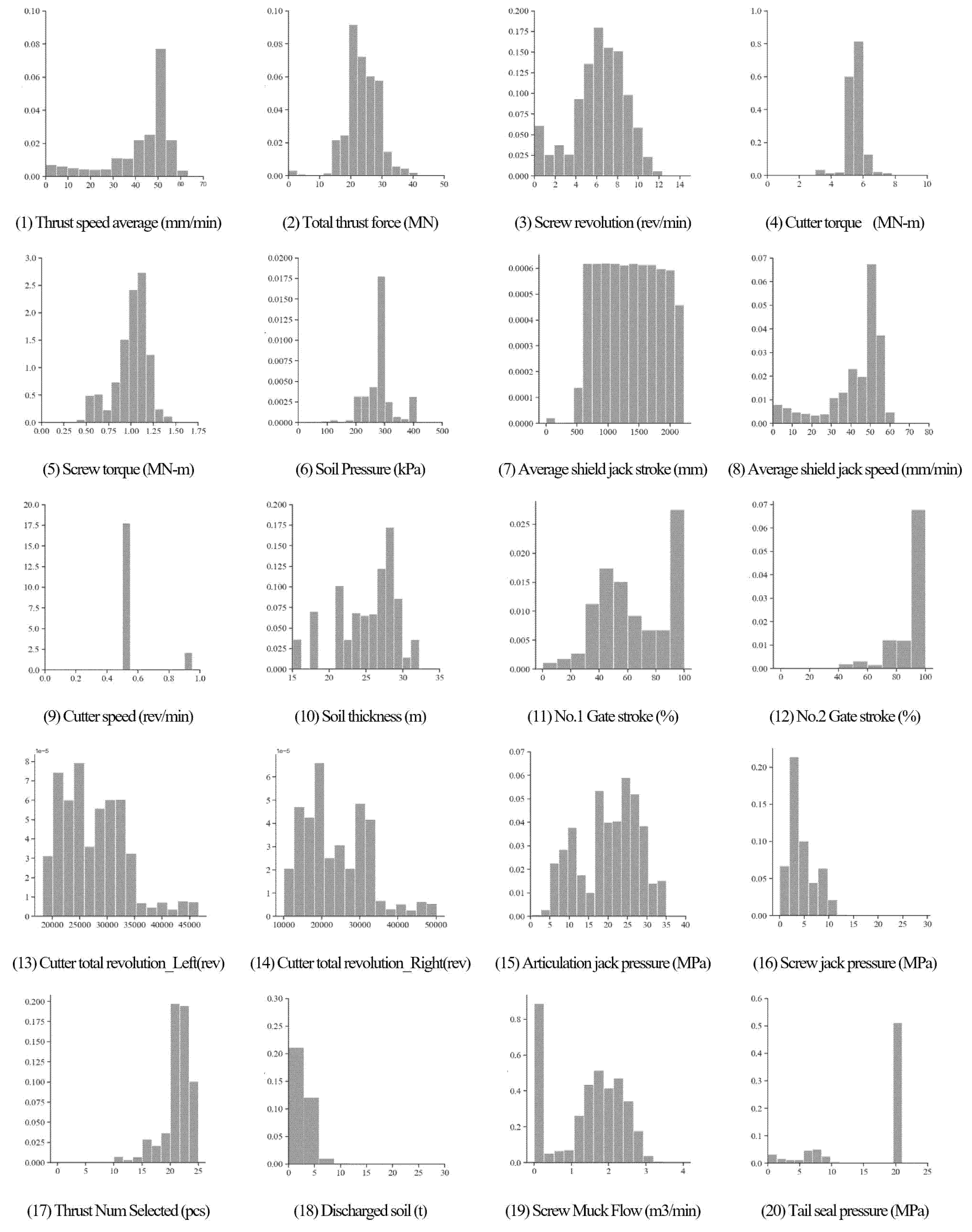
Among the 880 features of operating data generated during TBM excavation, features that do not affect classification prediction of this study (e.g., voltage, temperature, location, and attitude information) were excluded from the dataset. Correlations between 20 features (e.g., force, torque, rotational speed, speed, stroke, and pressure) measured at the cutterhead and TBM body were checked, and six representative features were then obtained considering all EPB-type TBM excavation sites.
In machine learning, since one feature is expressed as one axis during analysis, if there are many features for learning, the interpretation power of the machine learning model decreases. Therefore, in the data preparation stage for machine learning, it is necessary to reduce features, that is, to make the model intuitively easy to understand through dimension reduction.
This study selected the features with good statistical distribution to minimize the feature among the 20 features in Figure 2. Features with unbiased data were preferentially selected, and features with multicollinearity problems as shown in (8) of Figure 2 were excluded. From features (7)~(20) of Figure 2, the statistical distribution was not good (variation poor). Therefore, input variables with good statistical distribution were first selected for data-based learning, and six features were finally selected through correlation verification. The selected features were penetration rate, thrust force, cutterhead torque, screw torque, screw revolution speed, and earth pressure. The correlations of the selected features are shown in Figure 3 and a statistical analysis is summarized in Table 4.
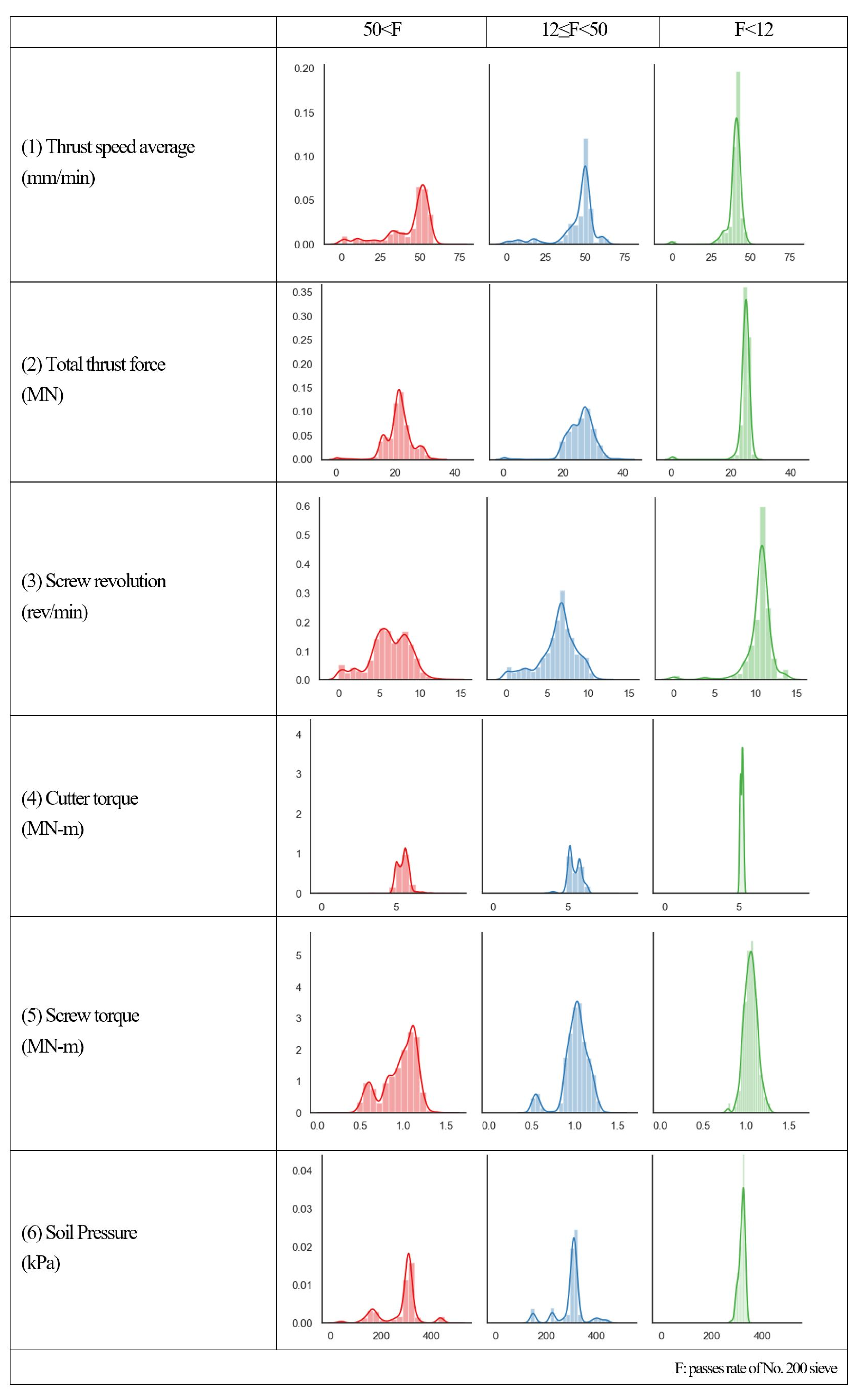
Mokhtari and Mooney [9] described that the machine data includes ground characteristics; Figure 4 shows that each feature has a different distribution depending on the ground characteristics. When the fine-soil component (particle diameter 0.075 mm) was small, (1) thrust speed average was a left-skewed distribution, whereas (2) thrust force was a right-skewed distribution. The peak of the distribution for (3) screw revolution shifted approximately from 5 to 11 rev/min. As the fine-soil component decreased, the distribution shape changed from a wide and low shape to a high and narrow shape for (4) cutter torque and (5) screw torque. (6) Soil pressure was maintained at about 287 kPa (Figure 4).
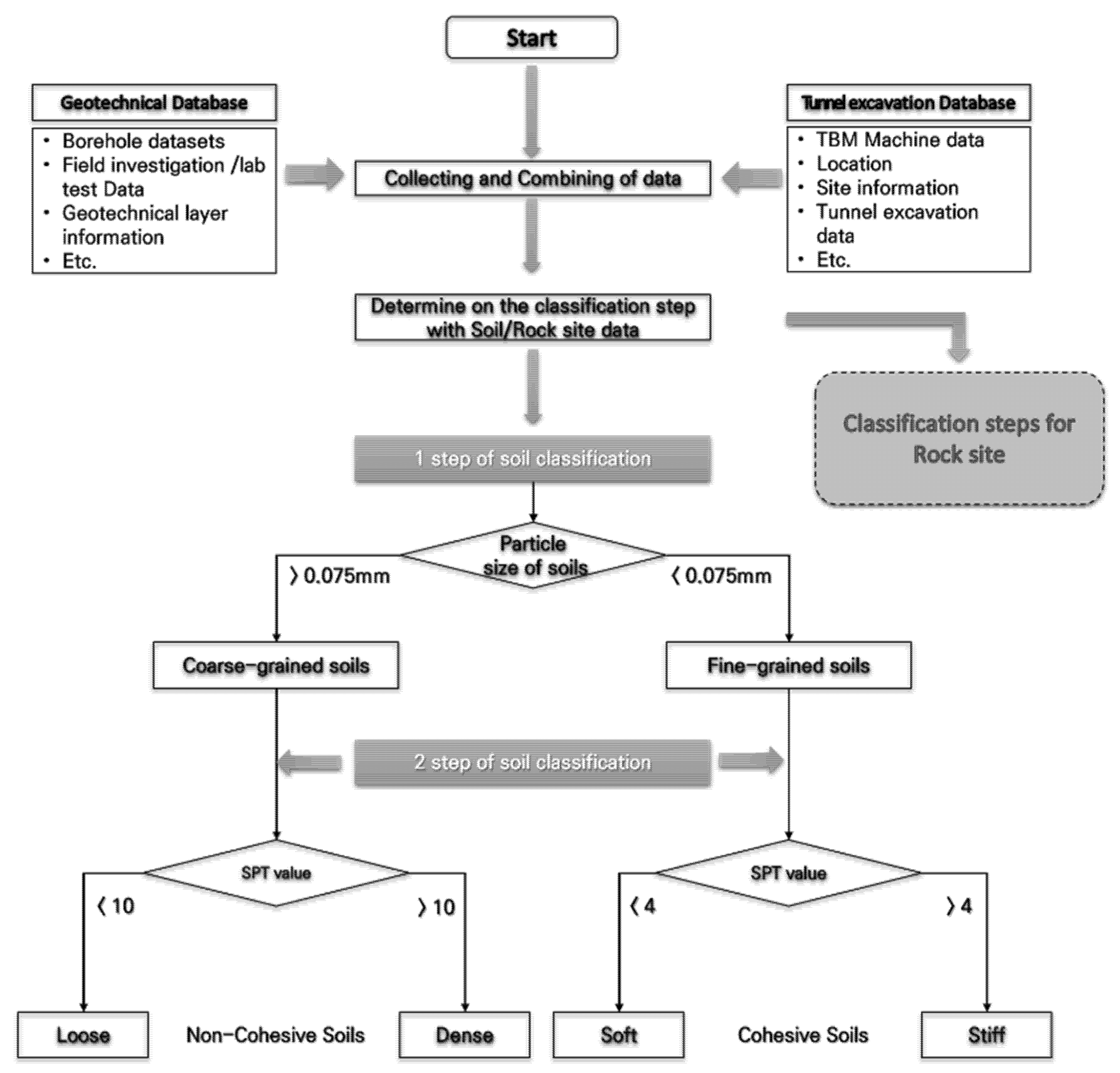
This study used a two-step model to predict soil classification (according to the ground characteristic criteria) using the operating data of the EPB-type TBM; the procedure is shown in Figure 5. Important factors selected for each stage of soil classification were the particle size of the soil used for the USCS and the N-value from SPT, which are described in Section 2.1 and Section 2.2, respectively.
The first step involved building a model that classifies coarse and fine soils based on the particle size (0.007 mm) in Table 1. In the second step, classification models were built using N-values according to the classification criteria in Table 2 for each dataset of coarse and fine soil classified in step 1. A Python 3.8 program and open source library (scikit-learn) were used for data analysis and machine learning. Figure 5 shows the detailed analysis and classification procedures.

4. Methodology

4.1. ML Models

4.1.1. Decision Tree

Decision tree is a method of classifying given data and finding rules. This model performs tree-based separation once to create an area that separates variables to obtain the desired class value. Decision tree techniques can be used for both continuous and categorical variables, and the effect on the dependent variable among many variables can be identified through the decision generation process such as dimension reduction or variable selection [23]. The tree technique is an efficient technique to discover characteristics by group or to identify and subdivide which category a group belongs to. It does not require preprocessing such as normalization or standardization of variables, and it can be used even if the value of a specific variable is omitted, but it has the disadvantage that it is difficult to generalize due to poor prediction performance when applied to new data due to overfitting characteristics.

4.1.2. Ensemble Learning Method (Boosting)

Ensemble models are models that generate and combine different classification algorithm models to extract optimal results. Typical examples include bootstrap aggregating (bagging) proposed by Breiman [24] and boosting (boosting) proposed by Kearns and Valiant [25] for the first time in classification algorithms. Bagging, which learns in various ways using duplicate samples, is a model that uses a single or multiple models in parallel, and in contrast, boosting is an algorithm that learns sequentially using a single model and performs re-learning by weighting the next classifier to secure the error that occurs.
AdaBoost (adaptive boost) is the most basic boost algorithm and has the advantage of being simple and efficient. It can be used in combination with many other types of learning algorithms to improve performance. The final result of the acceleration classifier can be represented by adding weight to the results of the wake learner. Using the AdaBoost learning algorithm, as learning progresses, more feature values that express the target object well can be acquired, creating a strong recognition algorithm [26].
Gradient boosting, also called GBM, is an algorithm introduced by Friedman [27], and AdaBoost obtains the final predictions with a linear sum considering the model weight, but GBM can obtain a more optimized result by obtaining the weight by gradient descent.
XG boost (extreme gradient boosting) is a GBM-based algorithm that optimizes existing systems with parallelization, tree pruning, and hardware optimization methods, and improves algorithm performance through normalization and missing value processing. Based on CART (classification and regression tree), this technique is available for both regression and classification, and includes regulations to prevent overfitting [28].
Light GBM is a GBM-based algorithm similar to XG boost, and it has a fast training speed and high efficiency by using a histogram-based algorithm. It uses the leaf-wise method to create complex models and increase accuracy, and has a faster and more similar performance compared to XG boost [29].

4.1.3. Support Vector Machine (SVM)

The support vector machine (SVM) is proposed by Vapnik [30], who is a mathmatician. The machine learning model is often utilized for pattern recognition and data analysis. In this model, supposing the characteristic of the dataset is represented as input parameters, sample data for learning are distributed in an n-dimensional data space. At this space, the SVM is the algorithm that finds the optimal boundary for classifying learning data. The principle of the SVM is to find a descision boundary with a maximum margin. The margin refers to the distance between the decision boundaries of the closest data points. Therefore, the classification of the SVM aims to find the boundaries that make the width of dividing the data class the largest within a certain margin error.

4.2. Modeling Methodology

A classification algorithm based on supervised learning is used to predict classification from the TBM’s operating data. A support vector machine and decision trees are used as single techniques. Four ensemble techniques are also considered: adaptive boost (AdaBoost), gradient boosting, extreme gradient boosting (XG boosting), and light gradient boosting machine (Light GBM). The first two ensemble methods are representative methods that use weak learning, and the second two compensate for the slow learning speed and overfittng problems of gradient boosting.
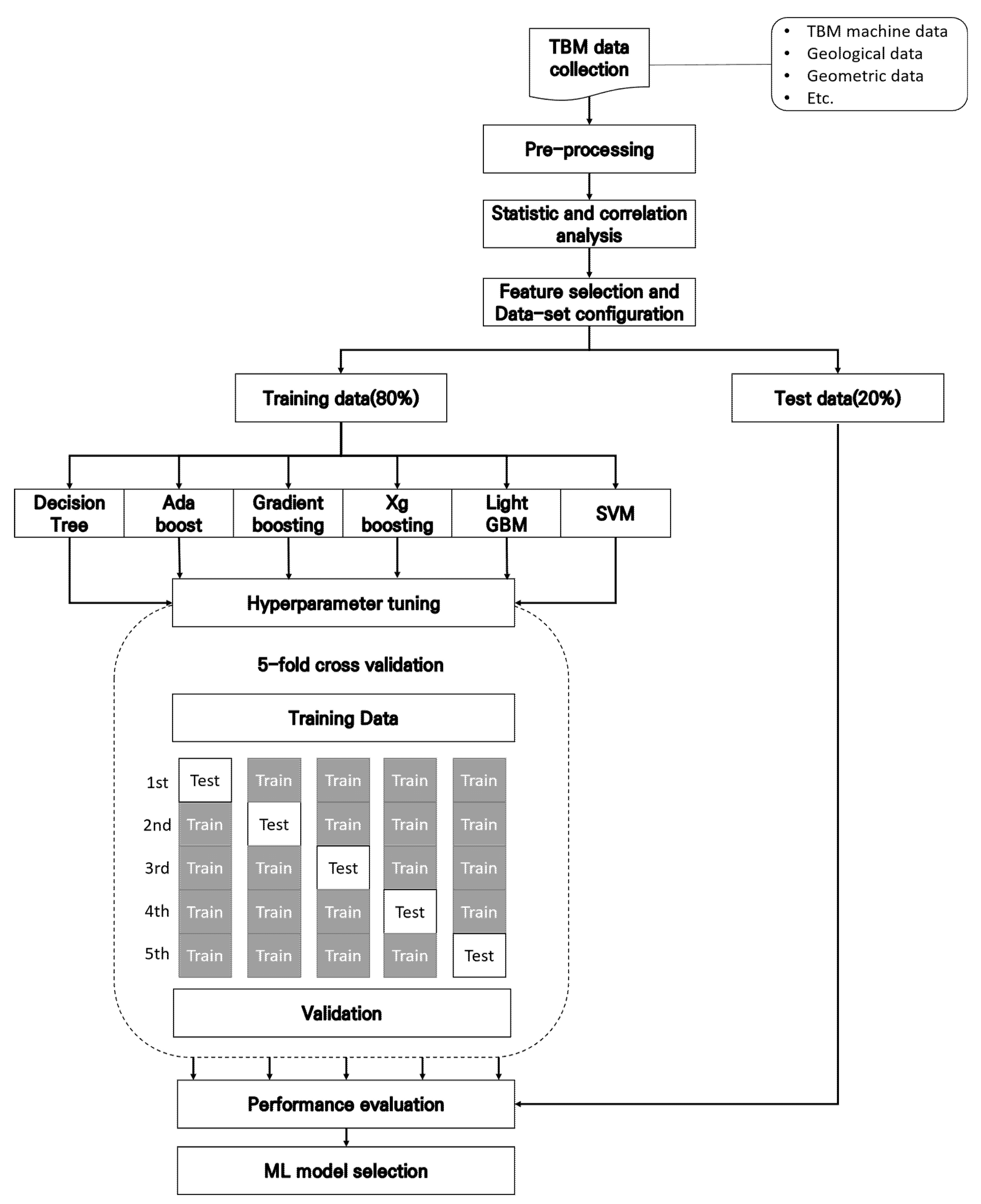
The entire data consisted of a training dataset for model learning and a test dataset that was not included in the training data to measure the accuracy of the model after training was completed. The ratio of training data and test data was 8:2. As a method to evaluate the prediction performance of the learned classification model, a confusion matrix showing the correct and incorrect answers of the classification model was used as shown in Table 5. Evaluation indicators such as accuracy, precision, recall, and F1-score were used to quantify and clearly confirm performance (Table 6). Figure 6 shows the overall flowchart of the machine learning process in this study.
TP + TN TP + TN + FP + FN
Standardization during data pre-processing was applied as re-scaling to prevent overfitting of the model. Missing values were treated by excluding any row with missing data, and a 95% confidence interval was established from the Z-distribution using the mean and standard deviation of the data. Outliers outside the confidence interval were removed.
The probability value (p-value) of the dataset was checked for the dataset after data pre-processing. It was found to be less than 0.05, which is the generally applied significance level in statistical hypothesis testing. To prevent overfitting that may occur when using a fixed training dataset and test dataset for model validation, k-fold cross validation, which can be used to evaluate any dataset, was applied. For the considered classification algorithms, GridSearchCV tuning was applied to find the best combination of hyperparameters based on performance comparison during training. Table 7 lists the parameters determined for each classification learning model.

5. Results

5.1. Classification Results by Soil Particle Size (Step 1)

The first step of soil classification in Figure 5 is classifying soil into three types. The first classification of fine or coarse by the USCS is completed using a No. 200 sieve (particle size 0.075 mm). If the amount of material passing through this sieve (F) is at least 50%, the soil is fine and classified as class 0. Lower pass rates indicate coarse soil, which is subdivided into class 1 (12% < F < 50%) and class 2 (F ≤ 12%) (Table 8).
Table 9 lists the results for each learning model using the above soil classification criteria. The accuracy value indicates how similar the predicted data are to the actual data, with values closer to 1 denoting better classification performance. In case there is an imbalance in the model class, the precision, recall, and F1-score should also be considered when assessing model performance (Table 6).
The decision tree and AdaBoost models have accuracy values of 0.759 and 0.781, respectively, indicating mediocre classification performance. The support vector machine and ensemble boosting models (i.e., gradient boosting, XG boosting, and Light GBM) have high accuracy values of at least 0.974; their other performance indicators (precision, recall, and F1-score) are also good. The classification performance results in the first stage of soil classification indicate the suitability of all four of these models.
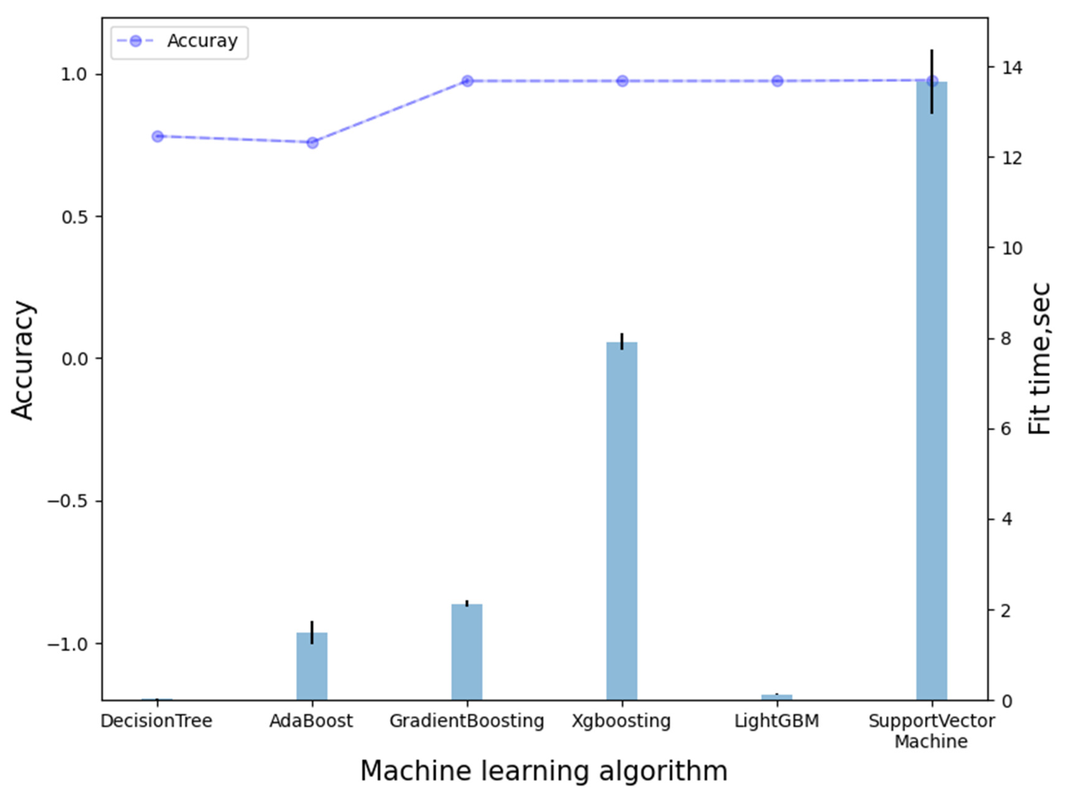
The support vector machine model shows the best performance, but it is slow to learn overall, especially in the hyperparameter determination process, and it requires significantly more computational resources than the other models. It is difficult to objectively calculate the computational resource consumption and learning speed of each model due to the number of hyperparameters to be adjusted and the characteristics of each model. However, conducting model learning on the same PC allows comparison of the learning time: in descending order of speed, the models are ranked Light GBM, XG boosting, gradient boosting, and support vector machine.
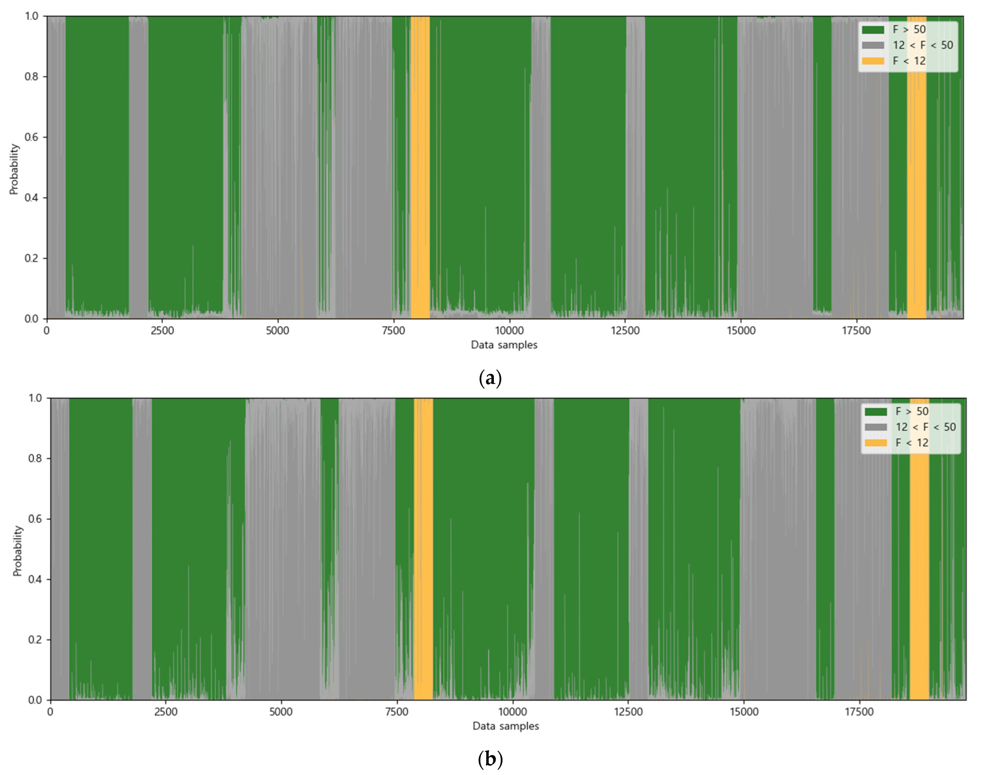
Prediction of step 1 classification for the entire dataset is compared using the support vector machine, the best-performing model, and Light GBM, the quickest-learning model (Figure 7). In each case, the three possible classes predict a probability (all three probabilities sum to 1), and the probability of each class is shown as the prediction results (Figure 7). As the dataset comprises only operating data for tunneling sections with known ground information, the order of the x-axis data in Figure 7 differs from the TBM excavation distance and the actual ground distances. The prediction results of the support vector machine and light GBM do not differ markedly, as shown in Figure 7.
Yagiz and Karahan [31] developed prediction models for estimating the performance of TBM using AI techniques. In this paper, they remarked that computational time and efficiency are critical factors in simulations using AI technology. To determine a suitable classification algorithm for this study, cross-validation is performed repeatedly by dividing all the data into five parts, and the average time taken for learning by each classification algorithm is then assessed, as shown in Figure 8.

5.2. Classification Results by N-Value (Step 2)

The second step of the classification model in Figure 5 is to subdivide the previously classified coarse and fine soil. This step uses the N-value from SPT to further classify coarse soil as dense or loose and fine soil as soft or stiff. The relevant ranges of the considered criterion, the N-value, differ depending on whether the soil is coarse or fine: non-cohesive (coarse) soil is classified using Table 2 as loose or dense based on a threshold N-value of 10, and cohesive (fine) soil is classified as stiff or soft relative to a threshold N-value of 5. Table 10 shows the classification classes in the second step.
Table 11 summarizes the performance of the models during step 2 in classifying soils previously categorized as cohesive or non-cohesive in step 1. The decision tree and AdaBoost show accuracy values of 0.835 and 0.879, respectively, for cohesive soils and 0.794 and 0.855, respectively, for non-cohesive soils. Similar to the performance in step 1 (Section 4.1), the single algorithm support vector machine and the ensemble boosting models gradient boosting, XG boosting, and Light GBM show higher accuracy values (here, at least 0.943), and their other performance indicators are also high.
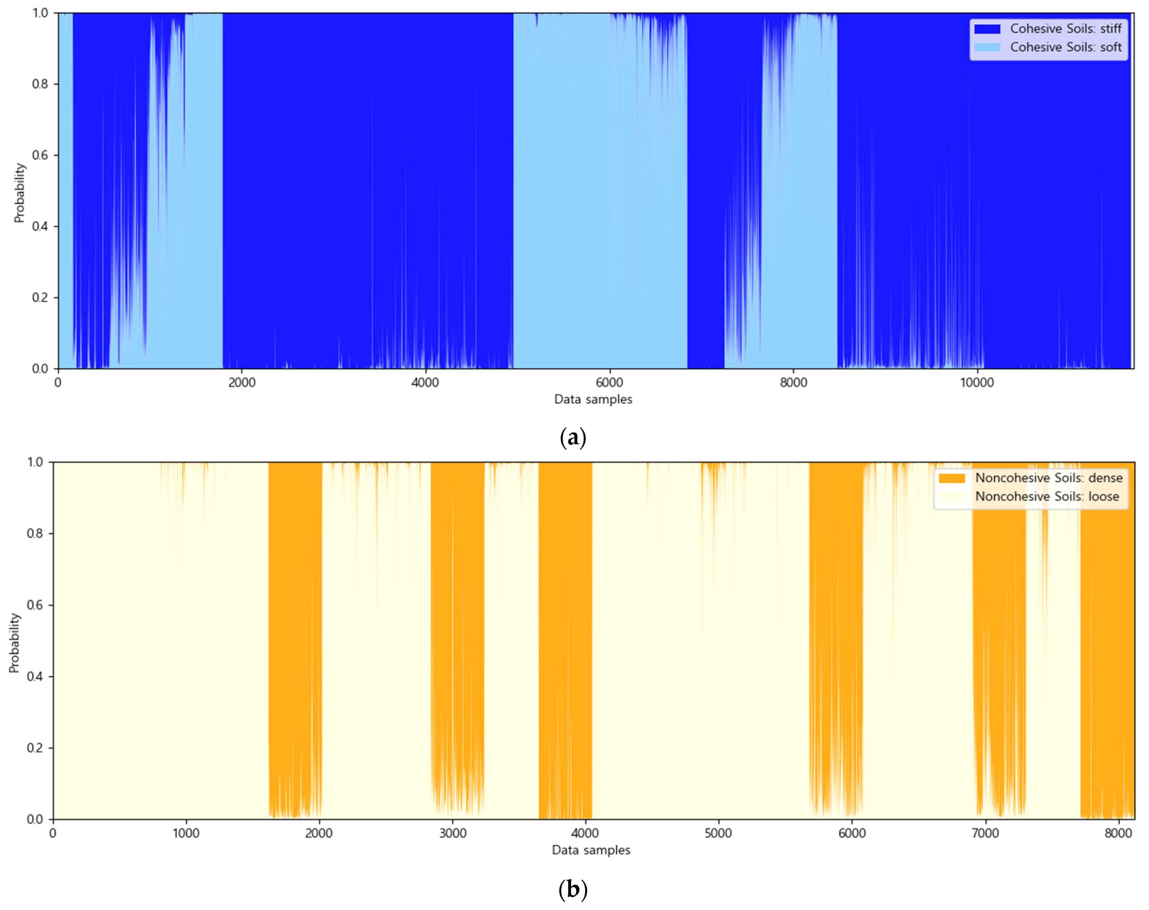
The four models with accuracy values of at least 0.943 have similar performance, so they can then be distinguished by their speed of operation on the same PC (as in Section 4.1). Light GBM is considered optimal, as it offers excellent classification performance and fast learning. Figure 9 shows the results of classifying and predicting the density and consistency of the entire learning dataset using Light GBM.

5.3. Classification Results for the Entire Dataset

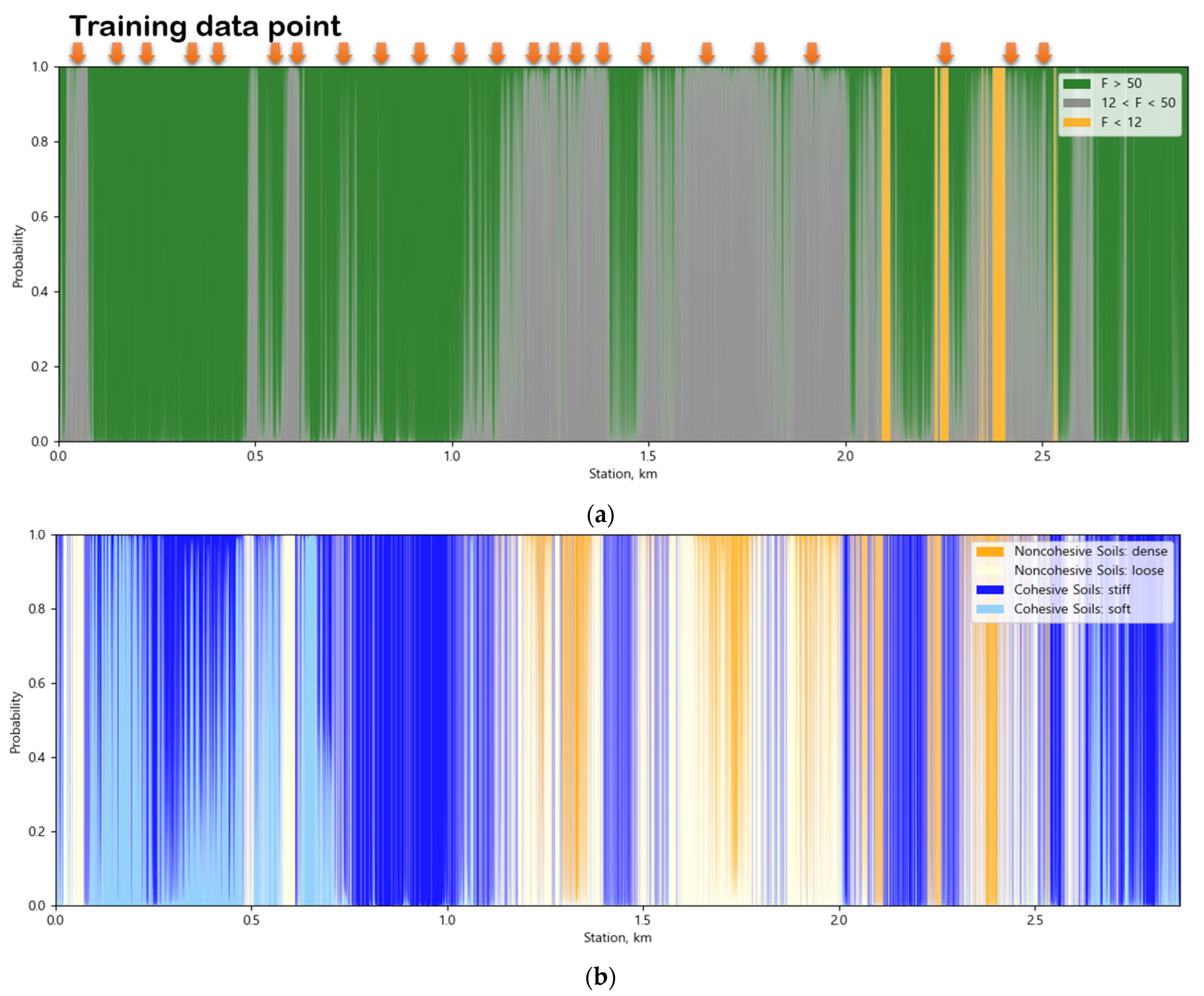
Various ground surveys, such as basic property tests, hydraulic characteristics tests, soft ground characteristics tests, and seismic exploration, are conducted when designing a tunnel, but ground information that could be used for actual TBM excavation is limited because most tests give results relevant only to the specific locality. Here, the soil classification for the entire excavation distance of the TBM is predicted using a model trained on the entire TBM machine data. The first classification (Section 5.1) divides the excavation data into coarse and fine soil (Figure 10a), and the states of the coarse and fine soils are further categorized based on the N-value in the second classification procedure (Figure 10b). This classification model can predict the distributions of coarse and fine soils and the conditions of those soils, even for sections lacking prior ground information data.

6. Conclusions

This study used machine learning to predict soil classification (following established standards) from the operating data of an earth-pressure shield TBM tunnel section. The classification had two stages: soil particle size and SPT results. The performances of various machine learning models were compared for each classification stage after learning found relationships between TBM operating data and geotechnical data.
Ground information for tunnel construction is relatively scarce compared with the amount of TBM excavation data; machine learning can use TBM data to predict soil classification (i.e., the No. 200 sieve pass rate and SPT N-value) when ground information from borehole surveys is lacking. This study considered classification models that use information that can be obtained in any tunneling situation, and thus soil classification could be predicted continuously during tunneling without requiring prior geotechnical surveys.
Feature selection in this study was achieved according to good or poor statistical distribution to minimize the features among the 20 features. There are various techniques for feature selection, such as those based on engineering judgment or using findings derived from existing studies, but there are also feature selection methods based on unsupervised learning that are recently used. The application of these techniques needs to be considered in future studies.
The process of classification prediction consists of data pre-processing and checking the probability value for the data, then composing training data and test datasets and applying cross-validation. The decision tree and AdaBoost models showed accuracy values of 0.759 to 0.879 in the first and second classification steps, but with poor precision and recall values of around 0.6. In contrast, the gradient boosting, XG boosting, Light GBM, and support vector models all showed excellent performance, with accuracy values over 0.90, and strong precision and recall values. The accuracy of machine learning results as well as the speed of learning are important factors to consider for the application of machine learning. Overall, Light GBM, which showed excellent learning performance and speed, is a suitable model for predicting soil classification based on EPB-type TBM excavation information.
This study intends to present the ground situation ahead with a higher probability to the constructor by using the TBM machine data that are continuously provided in real time during the TBM construction, which is performed with limited ground surveys. The classification model constructed here can be used to aid excavation in ground sections lacking prior information. However, the results of this study were derived based on data from a single site, and verification of data from various sites is required in the future.

Author Contributions

Conceptualization, T.-H.K. and S.-W.C.; methodology, S.-W.C.; software, T.-H.K.; validation, T.-H.K. and S.-W.C.; formal analysis, C.L. and S.-H.C.; investigation, T.-H.K., S.-W.C., C.L. and S.-H.C.; data curation, T.-H.K. and S.-W.C.; writing—original draft preparation, T.-H.K.; writing—review and editing, S.-W.C.; visualization, C.L. and S.-H.C.; supervision, S.-W.C.; project administration, S.-W.C.; funding acquisition, S.-H.C. All authors have read and agreed to the published version of the manuscript.

Funding

This research was conducted with the support of the National R&D Project for Smart Construction Technology (No. 22SMIP-A158708-03) funded by the Korea Agency for Infrastructure Technology Advancement under the Ministry of Land, Infrastructure, and Transport, and managed by the Korea Expressway Corporation.

Institutional Review Board Statement

Not applicable.

Informed Consent Statement

Not applicable.

Data Availability Statement

Not applicable.

Acknowledgments

The authors appreciate the support of the Korea Agency for Infrastructure Technology Advancement under the Ministry of Land, Infrastructure, and Transport, and managed by the Korea Expressway Corporation.

Conflicts of Interest

The authors declare no conflict of interest.

References

  1. Xu, H.; Zhou, J.; GAsteris, P.; Jahed Armaghani, D.; Tahir, M.M. Supervised Machine Learning Techniques to the Prediction of Tunnel Boring Machine Penetration Rate. Appl. Sci. 2019, 9, 3715. [Google Scholar]
  2. Liu, B.; Wang, Y.; Zhao, G.; Yang, B.; Wang, R.; Huang, D.; Xiang, B. Intelligent decision method for main control parameters of tunnel boring machine based on multi-objective optimization of excavation efficiency and cost. Tunn. Undergr. Space Technol. 2021, 116, 104054. [Google Scholar] [CrossRef]
  3. Salimi, A.; Rostami, J.; Moormann, C.; Delisio, A. Application of non-linear regression analysis and artificial intelligence algorithms for performance prediction of hard rock TBMs. Tunn. Undergr. Space Technol. 2016, 58, 236–246. [Google Scholar] [CrossRef]
  4. Ahangari, K.; Moeinossadat, S.R.; Behnia, D. Estimation of tunnelling-induced settlement by modern intelligent methods. Soils Found. 2015, 55, 737–748. [Google Scholar] [CrossRef] [Green Version]
  5. Chen, R.; Zhang, P.; Wu, H.; Wang, Z.; Zhong, Z. Prediction of shield tunneling-induced ground settlement using machine learning techniques. Front. Struct. Civ. Eng. 2019, 13, 1363–1378. [Google Scholar] [CrossRef]
  6. Mahdevari, S.; Shahriar, K.; Yagiz, S.; Shirazi, M.A. A support vector regression model for predicting tunnel boring machine penetration rates. Int. J. Rock Mech. Min. 2014, 74, 214–229. [Google Scholar] [CrossRef]
  7. Armaghani, D.J.; Mohamad, E.T.; Narayanasamy, M.S.; Narita, N.; Yagiz, S. Development of hybrid intelligent models for predicting TBM penetration rate in hard rock condition. Tunn. Undergr. Space Technol. 2017, 63, 29–43. [Google Scholar] [CrossRef]
  8. Gao, X.; Shi, M.; Song, X.; Zhang, C.; Zhang, H. Recurrent neural networks for real-time prediction of TBM operating parameters. Autom. Constr. 2019, 98, 225–235. [Google Scholar] [CrossRef]
  9. Mokhtari, S.; Mooney, M.A. Predicting EPBM advance rate performance using support vector regression modeling. Tunn. Undergr. Space Technol. 2020, 104, 103520. [Google Scholar] [CrossRef]
  10. Erharter, G.H.; Marcher, T.; Reinhold, C. Application of artificial neural networks for Underground construction–Chances and challenges–Insights from the BBT exploratory tunnel Ahrental Pfons. Geomech. Tunn. 2019, 12, 472–477. [Google Scholar] [CrossRef]
  11. Jung, J.-H.-H.; Chung, H.; Kwon, Y.-S.-S.; Lee, I.-M.-M. An ANN to Predict Ground Condition ahead of Tunnel Face using TBM Operational Data. KSCE J. Civ. Eng. 2019, 23, 3200–3206. [Google Scholar] [CrossRef]
  12. Zhuang, D.Y.; Ma, K.; Tang, C.A.; Liang, Z.Z.; Wang, K.K.; Wang, Z.W. Mechanical parameter inversion in tunnel engineering using support vector regression optimized by multi-strategy artificial fish swarm algorithm. Tunn. Undergr. Space Technol. 2019, 83, 425–436. [Google Scholar] [CrossRef]
  13. Zhang, Q.L.; Hu, W.F.; Liu, Z.Y.; Tan, J.R. TBM performance prediction with Bayesian optimization and automated machine learning. Tunn. Undergr. Space Technol. 2020, 103, 103493. [Google Scholar] [CrossRef]
  14. Ayawah, P.E.; Sebbeh-Newton, S.; Azure, J.W.; Kaba, A.G.; Anani, A.; Bansah, S.; Zabidi, H. A review and case study of Artificial intelligence and Machine learning methods used for ground condition prediction ahead of tunnel boring Machines. Tunn. Undergr. Space Technol. 2022, 125, 104497. [Google Scholar] [CrossRef]
  15. Xue, Y.D.; Zhao, F.; Zhao, H.X.; Li, X.; Diao, Z.X. A new method for selecting hard rock TBM tunnelling parameters using optimum energy: A case study. Tunn. Undergr. Space Technol. 2018, 78, 64–75. [Google Scholar] [CrossRef]
  16. Yang, H.; Song, K.; Zhou, J. Automated recognition model of geomechanical information based on operational data of tunneling boring machines. Rock Mech. Rock Eng. 2022, 55, 1499–1516. [Google Scholar] [CrossRef]
  17. Terzaghi, K.; Peck, R.B. Soil Mechanics in Engineering Practice; John Wiley and Sons: New York, NY, USA, 1948. [Google Scholar]
  18. Brown, T.; Hettiarachchi, H. Estimating Shear Strength Properties of Soils Using SPT Blow Counts: An Energy Balance Approach; ASCE Geotechnical Special Publication No. 179; ASCE: Reston, VA, USA, 2008. [Google Scholar] [CrossRef]
  19. Kulhawy, F.H.; Mayne, P.W. Manual on Estimating Soil Properties for Foundation Design; Electric Power Research Institute: Palo Alto, CA, USA, 1990. [Google Scholar]
  20. Peck, R.B.; Hanson, W.E.; Thornburn, T.H. Foundation Engineering, 2nd ed.; Wiley: New York, NY, USA, 1974. [Google Scholar]
  21. Terzaghi, K.; Peck, R.B. Soil Mechanics in Engineering Practice, 2nd ed.; Wiley: New York, NY, USA, 1967. [Google Scholar]
  22. Peck, R.B.; Hanson, W.E.; Thornburn, T.H. Foundation Engineering; John Wiley & Sons: New York, NY, USA, 1953; p. 410. [Google Scholar]
  23. Breiman, L.; Friedman, J.; Stone, C.J.; Olshen, R.A. Classification and Regression Trees; CRC Press: Boca Raton, FL, USA, 1984. [Google Scholar]
  24. Breiman, L. Bagging predictors. Mach. Learn. 1996, 24, 123–140. [Google Scholar] [CrossRef] [Green Version]
  25. Kearns, M.; Valiant, L.G. Cryptographic limitations on learning Boolean formulae and finite automat. J. Assoc. Comput. Mach. 1994, 41, 67–95. [Google Scholar] [CrossRef]
  26. Freund, Y.; Schapire, R. A decision theoretic generalization of on-line learning and an application to boosting. J. Comput. Syst. Sci. 1997, 55, 119–139. [Google Scholar] [CrossRef] [Green Version]
  27. Friedman, J.H. Greedy function approximation: A gradient boosting machine. Ann. Stat. 2001, 29(5), 1189–1232. [Google Scholar] [CrossRef]
  28. Chen, T.; He, T.; Benesty, M.; Khotilovich, V.; Tang, Y.; Cho, H.; Chen, K. Xgboost: Extreme Gradient Boosting; R Package Version 0.4-2 1.4; 2015; pp. 1–4. Available online: https://cran.r-project.org/web/packages/xgboost/vignettes/xgboost.pdf (accessed on 10 October 2022).
  29. Ke, G.; Meng, Q.; Finley, T.; Wang, T.; Chen, W.; Ma, W.; Ye, Q.; Liu, T.Y. Lightgbm: A highly efficient gradient boosting decision tree. Adv. Neural Inf. Process. Syst. 2017, 30. [Google Scholar]
  30. Vapnik, V.N. The Nature of Statistical Learning Theory; Springer: New York, NY, USA, 1995. [Google Scholar] [CrossRef]
  31. Yagiz, S.; Karahan, H. Application of various optimization techniques and comparison of their performances for predicting TBM penetration rate in rock mass. Int. J. Rock Mech. Min. Sci. 2015, 80, 308–315. [Google Scholar] [CrossRef]
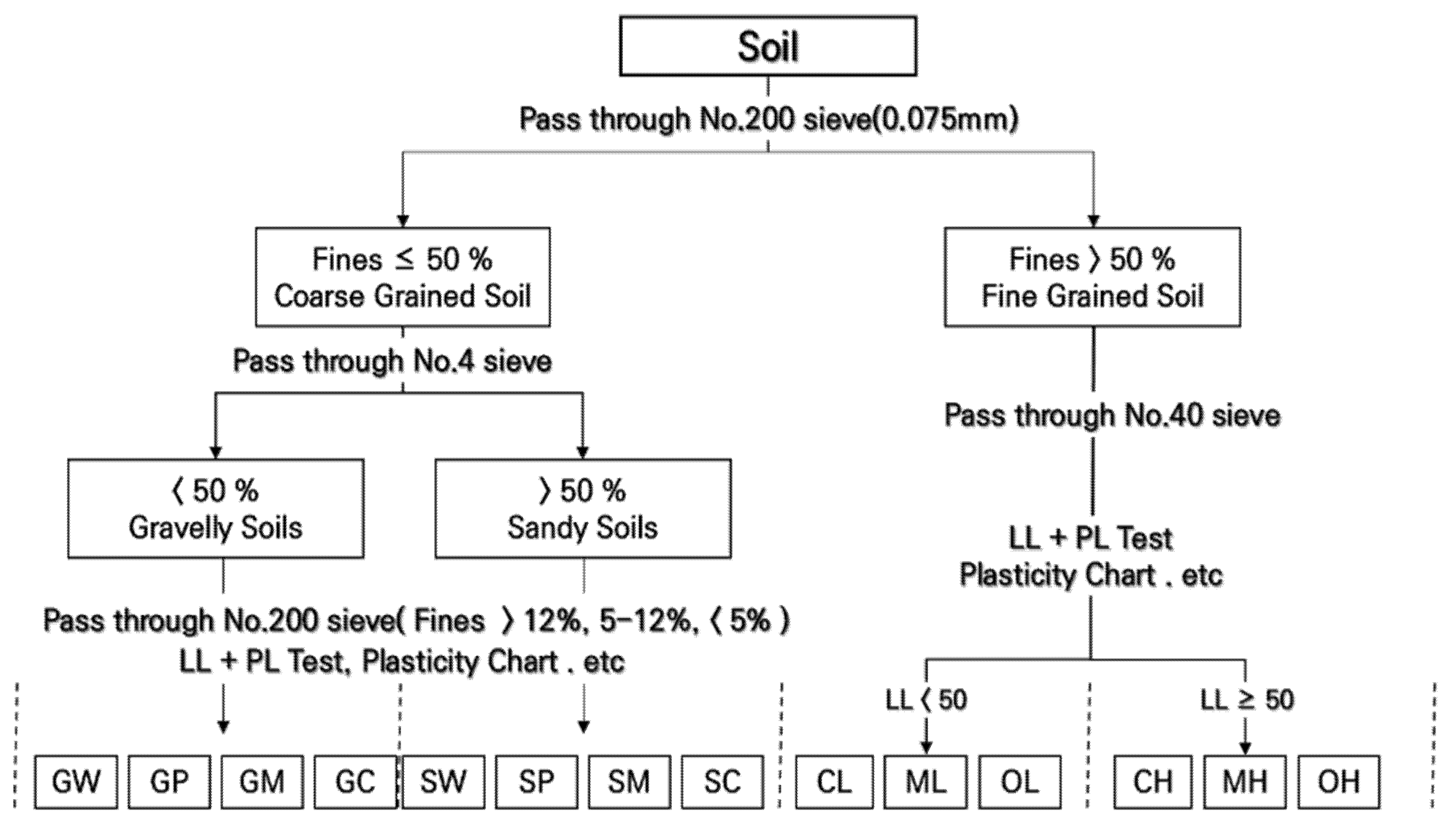
Figure 1. Soil classification of the Unified Soil Classification System.
Applsci 12 11480 g001
Figure 2. Distribution of data for feature selection.
Applsci 12 11480 g002
Figure 3. Pair-wise correlations between features of TBM data.
Applsci 12 11480 g003
Figure 4. Distribution of data according to ground conditions for data features.
Applsci 12 11480 g004
Figure 5. Soil classification procedure for the classification model.
Applsci 12 11480 g005
Figure 6. Flowchart of machine learning model procedure for class prediction.
Applsci 12 11480 g006
Figure 7. Prediction results by classification model (step 1: particle size): (a) support vector machine; (b) Light GBM.
Applsci 12 11480 g007
Figure 8. Summary of accuracy and fit times for cross-validation.
Applsci 12 11480 g008
Figure 9. Prediction results by classification models (step 2: N-value): (a) cohesive soils; (b) non-cohesive soils.
Applsci 12 11480 g009
Figure 10. Classification results for the entire dataset: (a) classification step 1 (particle size); (b) classification step 2 (SPT value).
Applsci 12 11480 g010
Table 1. Summary of particle size classification using the Unified Soil Classification System.
USCS ClassificationParticle Size (mm)
Gravel76.2~4.75
Sand4.75~0.075
Silt<0.075
Clay<0.002
Table 2. Density and consistency of soil derived from standard penetration testing [22].
Cohesive SoilsNon-Cohesive Soils
NConsistencyNDensity
<2Very soft0~4Very loose
2~4Soft
4~8Medium4~10Loose
8~15Stiff10~30Medium dense
16~32Very stiff
>32Hard30~50Dense
50<Very dense
Table 3. Summary of TBM specifications.
TBM TypeEPB
TBM outside diameter (m)7.9
Max. shield jack thrust force (MN)50 (2 × 25 shield jack)
Max. cutterhead torque (MN·m)9.6
Max. RPM (rev/min)0.89
Max. screw revolution (rev/min)14.2
Segment ring length (m)1.2
Table 4. Statistical description of the database.
FactorsMinQ1 (25%)Q2 (50%)Q3 (75%)MaxAverageStandard Deviation
(1)Thrust speed average
     (mm/min)
03849527342.214.6
(2) Total thrust force
     (MN)
020.723.327.441.423.75.4
(3) Screw revolution
     (rev/min)
02.45.97.714.25.23.3
(4) Cutter torque
     (MN-m)
05.185.555.819.015.50.62
(5) Screw torque
     (MN-m)
00.921.041.131.561.00.19
(6) Soil pressure
     (kPa)
27289306314496287.762.4
Table 5. Confusion matrix of classification.
ClassPositive (1)Negative (0)
Positive (1)True Positive (TP)False Positive (FP)
Negative (0)False Negative (FN)True Negative (TN)
Table 6. Classification performance measures.
Formulas for Measuring
Performance
Definition of the Terms
Accuracy TP + TN TP + TN + FP + FN Accuracy is the proportion of the total number of predictions that are correct
Precision TP TP + FP Precision is the ratio of the total number of correctly classified positive examples and the total number of predicted positive examples
Recall TP TP + FN Recall is also referred to as true positive rate or sensitivity
F1-score 2 × Precision × Recall Precision + Recall F1-score is a weighted average of the recall (sensitivity) and precision
Table 7. Summary of the hyperparameters of the algorithms.
AlgorithmHyperparameter
Tree-Based MethodsDecision Treemax depth: 5
Ensemble Learning Method, BoostingAdaBoostlearning rate: 0.1, n estimators: 300
Gradient Boostinglearning rate: 0.5, max depth: 4, max features: 3,
n estimators: 500
XG boostinglearning rate: 0.2, max depth: 4, n estimators: 400
Light GBMlearning rate: 0.1, max depth: 5, n estimators: 300
Support Vector MachineSVMC: 2.0, gamma: 2.8
Table 8. Criteria for classification in step 1.
Class RangeDescription
0* F ≥ 50Fine-Grained Soil
112 < F < 50Coarse-Grained Soil
2F ≤ 12%
* F is the percentage of soil passing through a No. 200 sieve (0.075 mm).
Table 9. Evaluating classification performance (step 1) for EPB TBM datasets.
ModelTest Dataset
AccuracyPrecisionRecallF1-Score
Decision Treeclass 00.7810.770.890.83
class 10.770.60.68
class 20.950.830.89
AdaBoostclass 00.7590.760.870.81
class 10.730.570.64
class 20.910.910.91
Gradient Boostingclass 00.9740.980.980.98
class 10.970.970.97
class 20.960.960.96
XG boostingclass 00.9740.980.980.98
class 10.970.960.97
class 20.970.970.97
Light GBMclass 00.9740.980.980.98
class 10.970.960.97
class 20.960.950.96
Support Vector Machineclass 00.9770.980.980.98
class 10.980.970.97
class 20.960.960.96
Table 10. Criteria for classification in step 2.
Class RangeDescription
Cohesive SoilsNon-Cohesive Soils
0N ≥ 5stiffN > 10dense
1N < 5softN ≤ 10loose
Table 11. Evaluation of classification performance (step 2) for EPB TBM datasets.
ModelTest Dataset
Cohesive SoilsNon-Cohesive Soils
AccuracyPrecisionRecallF1-ScoreAccuracyPrecisionRecallF1-Score
Decision Treeclass 00.8350.840.940.890.7940.800.430.56
class 10.820.610.700.800.960.87
AdaBoostclass 00.8790.870.970.920.8550.860.650.74
class 10.910.690.780.870.950.91
Gradient
Boosting
class 00.9550.960.970.970.9630.940.940.94
class 10.930.920.930.970.970.97
XG Boostingclass 00.9560.960.970.970.9640.940.940.94
class 10.940.920.930.980.980.97
Light GBMclass 00.9560.970.970.970.9620.940.940.94
class 10.930.930.930.970.970.97
Support Vector Machineclass 00.9430.950.930.930.9630.940.930.94
class 10.920.900.910.970.980.97
Publisher’s Note: MDPI stays neutral with regard to jurisdictional claims in published maps and institutional affiliations.