Article

FGCM: Noisy Label Learning via Fine-Grained Confidence Modeling

1
College of Biomedical Engineering and Instrument Science, Zhejiang University, Hangzhou 310007, China
2
Zhejiang Provincial Key Laboratory for Network Multimedia Technologies, Hangzhou 310007, China
3
Zhejiang University Embedded System Engineering Research Center, Ministry of Education of China, Hangzhou 310007, China
*
Author to whom correspondence should be addressed.
Appl. Sci. 2022, 12(22), 11406; https://doi.org/10.3390/app122211406
Submission received: 29 September 2022 / Revised: 1 November 2022 / Accepted: 3 November 2022 / Published: 10 November 2022
(This article belongs to the Special Issue Advances in Deep Learning III)

Abstract

:
A small portion of mislabeled data can easily limit the performance of deep neural networks (DNNs) due to their high capacity for memorizing random labels. Thus, robust learning from noisy labels has become a key challenge for deep learning due to inadequate datasets with high-quality annotations. Most existing methods involve training models on clean sets by dividing clean samples from noisy ones, resulting in large amounts of mislabeled data being unused. To address this problem, we propose categorizing training samples into five fine-grained clusters based on the difficulty experienced by DNN models when learning them and label correctness. A novel fine-grained confidence modeling (FGCM) framework is proposed to cluster samples into these five categories; with each cluster, FGCM decides whether to accept the cluster data as they are, accept them with label correction, or accept them as unlabeled data. By applying different strategies to the fine-grained clusters, FGCM can better exploit training data than previous methods. Extensive experiments on widely used benchmarks CIFAR-10, CIFAR-100, clothing1M, and WebVision with different ratios and types of label noise demonstrate the superiority of our FGCM.

1. Introduction

The double-edged nature of deep neural networks’ tremendous capacity to learn and memorize data has been revealed [1,2,3]. However, although DNNs trained on large-scale datasets achieved massive success in image classification [4], object detection [5], and other visual tasks, they tend to undesirably memorize random false-labeled samples [3], resulting in poor generation ability. Currently, there is growing research interest in noisy label learning [6,7,8,9,10,11,12,13] owing to the scarcity of large-scale datasets with high-quality annotations in most real-world cases [14]. Recent methods for noisy label learning [6,8,12,15,16,17,18,19] are mostly inspired by the experimental observation [3] that DNNs tend to learn patterns existing among samples early and later struggle to memorize hard samples. These methods divide clean samples from noisy ones by treating samples with higher prediction confidence as clean instances while others as noisy instances [1]. For example, MentorNet [16] trains a student network by feeding in small-loss samples selected by a teacher model. Co-teaching [17] and co-teaching+ [18] train two DNNs parallelly, where each network provides small-loss samples to the other. Mcorr [8] estimates the probability of a sample being clean by fitting a two-component beta mixture model on prediction loss. Here, a more robust representation can be learned by excluding samples with low certainty of being clean from further training.
However, the performance of the methods above is limited because it leaves many unused mislabeled and hard samples that contain helpful information [2]. Therefore, we rethink confidence modeling from a more fine-grained perspective of considering the difficulty experienced by DNN models when learning from samples. Most existing methods overlook the different properties between hard and simple instances. Simple samples have easily identifiable features, while hard samples are rather indistinct. Here, instead of dividing the training data into either clean or noisy, we naturally categorize samples into four kinds: Clean Simple(CS), Noisy Simple(NS), Clean Hard(CH), and Noisy Hard. The Noisy Hard set is further divided into samples with relevant annotations (NHR) and irrelevant labels (NHI). Figure 1 presents the significant differences among the confidence trends of typical examples for each category during the training process, indicating the feasibility of fine-grained categorization. Furthermore, it can be inferred from Figure 1 that the confidence scores of maximum repeating pseudo labels share the same or similar trends with those of ground truth labels during the early training stage for all the five clusters. Thus, we use the former as an alternative when generating sample categories for the latter because the latter is not available in real-world cases.
In this paper, we aim to robustly train deep neural networks on noisily labeled datasets by recalling as much reusable training samples as possible. As mentioned above, existing sample selection methods treat samples with higher prediction confidence as clean instances. In this way, only a small portion of data can be selected. Moreover, it is hard to distinguish hard samples from noisy samples, both having low prediction confidence. Therefore, inspired by the findings induced from Figure 1, we propose a simple yet effective Fine-Grained Confidence Modeling (FGCM) framework. First, FGCM clusters samples into the five categories mentioned above by modeling the prediction scores for both annotations and the maximum repeating pseudo labels of samples. Second, to include as many clean and reusable samples in training, FGCM applies different strategies to different categories. In particular, we take data from CS and CH as it is, correct labels from NS to the maximum repeating pseudo labels, since there is a high possibility for the maximum repeating pseudo labels of NS instances to be correct according to Figure 1, and drop the labels of NHI together with NHR which are ambiguous. By iteratively repeating the process, FGCM can effectively prevent models from over-fitting to false-labeled samples and gradually recall more reusable samples from dropped data to further strengthen the performance of the trained model. Finally, semi-training strategy is employed to realize the use of NHI and NHR sets, enhancing the performance of trained model. With the fine-grained categorization of samples, FGCM can maximize the use of the training data.Extensive experiments on various datasets show that FGCM outperforms SOTA methods.
Our main contributions are summarized as follows:
  • We propose fine-grained training sample categories based on the difficulty of learning them and their label correctness.
  • We propose a simple yet effective FGCM framework for noisy label learning, which can effectively maximize the useation of the training data and prevent models from over-fitting to noisy labels.
  • Extensive experiments show the effectiveness and robustness of FGCM under different ratios and types of noise, outperforming previous methods.

2. Related Work

In this section, we briefly review the existing literature on noisy label learning. As listed in Table 1, previous methods can be grouped into several categories.
Noise transition matrix. Many early studies tackle the task of noisy label learning by estimating a noise transition matrix which represents the probability of one class being mislabeled into another. Some methods try to improve the performance by adjusting the prediction results of DNNs using the estimated label transition probability. Other methods, such as Fcorr [20], correct the loss by multiplying the estimated transition probability with the softmax outputs. The key to these methods is the reliability of the estimated noise transition matrix. Webly learning  [21] estimates a noise transition matrix by training an additional noise adaptation layer. Probabilistic noise modeling  [22] trains two networks which are used to predict the noise type and label transition probability, respectively.
The performance of these methods is often limited in realistic cases due to the complexity of estimating noise transition matrix on real-world datasets.
Robust Loss Function. Some studies try to design noise tolerant loss functions. The robust MAE [23] showed that the mean absolute error (MAE) loss is more robust to label noise than cross entropy (CE) loss, yet it is not applicable on complicated real world datasets and suffered from increased difficulty in training compared with cross entropy loss. Thus, the generalized cross entropy (GCE) [24] is introduced, trying to combine the advantages of both MAE and CE loss. Symmetric cross entropy (SCE) [25] proposes a noise robust term called reverse cross entropy loss, which can improve the learning on hard classes. SCE archives significantly better performance than CE and GCE. However, the accuracy of these loss function methods is still not promising and their performance will be greatly degraded in hard cases.
Sample Selection. Many recent studies adopted sample selection strategies which select a certain number of possibly clean labeled samples from the training dataset and exclude other samples from the update to prevent the model from over-fitting to noisy labels. The small-loss trick is widely used to distinguish true-labeled samples from noisy samples because the losses of clean samples tend to be smaller than false-labeled samples due to the memorization effect of DNNs. MentorNet [16] trains a student network by feeding in small-loss samples selected by a teacher model. Co-teaching [17] and Co-teaching+ [18] train two networks simultaneously and each network selects small-loss samples for the training of the other model. Iterative-CV [26] randomly divides training samples into subsets and iteratively removes samples with large losses using a cross validation strategy. Despite the significant improvements these methods obtain, samples acquired by them are mostly clean simple instances. Hard samples containing rich information which can greatly help the generalization of DNNs are discarded. Moreover, in extreme circumstances where the noise rate is high, too few samples can be selected to train the model thoroughly. Last but not least, the ground truth noise rate or a clean validation dataset, which are not available in most cases, need to be provided to decide how many samples should be selected.
Hybrid Methods. Recent studies attempted to combine sample selection with other techniques. SELF [27] uses the mean-teacher model to progressively filter out noisy samples. Mcorr [8] proposes to fit a two-component mixture model on prediction loss to estimate the probability of a sample being clean or noisy. Following Mcorr, DivideMix [19] divides training samples into a clean or noisy set using the obtained probabilities. Then semi-supervised learning is performed with instances in the clean set treated as labeled data while those in noisy set as unlabeled data.
There are some methods try to alleviate the effect of noisy labels using supervised contrastive learning techniques. MOIT+ [28] pretrains models with supervised contrastive learning. Then the learned features are used to divide samples into clean or noisy. Then a classifier is trained in a semi-supervised manner on the divided datasets. Sel-CL+ [12] achieves approximately 10% higher accuracy than MOIT+ on severely noisy datasets by pretraining models with unsupervised contrastive learning to completely remove the impact of noisy labels. Then, Sel-CL+ uses the learned low-dimensional representations to select confident pairs of samples for the supervised contrastive training of models instead of selecting confident samples as MOIT+ does. In this way, Sel-CL+ is able to leverage supervised information from not only the pairs with correct annotations, but also the pairs which are false-labeled from the same class.
Although these methods achieved promising performance, the improvements mostly are mostly owed to the using of semi-supervised or contrastive learning techniques. As with traditional sample selection methods, they still leave a large part of helpful supervisory signal unused, particularly from large loss training samples which consist of noisy labeled samples and hard samples.

3. Proposed Method

In this section, in detail, we introduce FGCM, our proposed training framework for learning from noisy labels. In summary, FGCM consists of three steps. (a) Generating fine-grained sample clusters based on their confidence trends. (b) Performing cluster refinement to promote the accuracy of sample clusters and constructing a cleaned training set with samples from CS, CH, and NS sets. Step (a) and (b) are iteratively repeated in the training process to expand the cleaned training set. (c) Performing mixed semi-training with instances from NHI and NHR sets treated as unlabeled data and instances in the cleaned training set as labeled data to maximum the use of training samples. The three steps will be introduced in detail in the following subsections.
First, to avoid confusion, we define the notations of the three kinds of labels which will be frequently mentioned for the rest of the paper. Annotation labels, denoted as AY = { a y 1 , a y 2 , , a y n } , are the assigned labels of samples, part of which are false-labeled while others are correct. GY = { g y 1 , g y 2 , , g y n } refers to ground truth labels which are the correct labels of samples. Maximum repeating pseudo labels MY = { m y 1 , m y 2 , , m y n } are the most frequent pseudo labels for each sample predicted by DNNs from the beginning of training to the current epoch.

3.1. Generalization of Sample Clusters

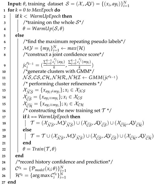
The process of generating sample clusters and performing cluster refinements is presented in Algorithm 1 which is located in page 6. Let S = ( X , AY ) = { ( x i , a y i ) } i = 1 N denote the training set consists of N samples, where x i is an input image with a y i being the corresponding annotation label. To obtain the maximum repeating pseudo label m y i for sample x i , we need to record the history prediction confidence for every sample as C e k . Given a model with parameter θ , the confidence score c i e k ( y ˜ ) represents the probability of sample i to be classified into class y ˜ after kth epoch of training:
c i e k ( y ˜ ) = P m o d e l y ˜ ( x i ; θ e k )
where P m o d e l y ˜ refers to the model’s output softmax probability for class y ˜ . We also maintain a history prediction list H e k which contains the pseudo labels produced by the model for each sample from the beginning of the training process to the current epoch k:
H e k = { { arg max P m o d e l ( x i ; θ e j ) } i = 1 N } j = 0 k
where arg max P m o d e l ( x i ; θ e j ) refers to the predicted label with maximum confidence, as known as the pseudo label, for sample i in epoch j. We use the label with maximum number of occurrences in H i e k as m y i for sample i. The model is trained on the whole training set in the early stage when the impact of noisy labels is minor. After the warmup phase ends, a joint confidence score j c i e k 1 is constructed for sample i in every epoch k:
j c i e k 1 = ( j = 0 k 1 c i e j ( a y i ) k , j = 0 k 1 c i e j ( m y i ) k )
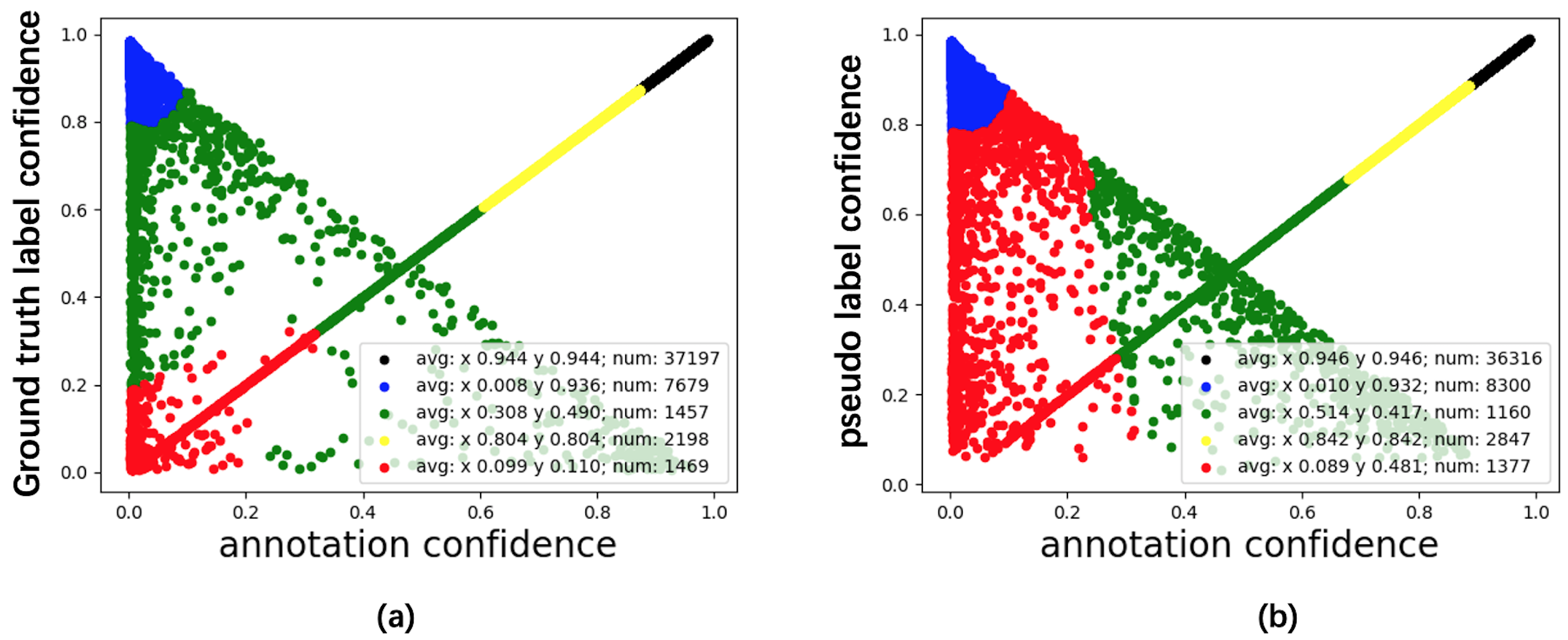
The two elements in j c i e k 1 represent the average of historical prediction confidence for annotation and maximum repeating pseudo label, respectively, reflecting the trends of their confidence scores during the training process. Gaussian Mixture Model (GMM) [29] is a widely used unsupervised modeling technique. A Gaussian Mixture Model is a weighted sum of M component Gaussian densities, where M is the number of clusters in the data. GMM assumes that the input data points are generated from a mixture of M Gaussian distributions. With parameter estimation using the Expectation-Maximization algorithm [30], GMM outputs the probabilities of samples belonging to each cluster. In this paper, we categorize samples into the cluster with maximum possibility. Owing to the different trends showed in Figure 1, five clusters of sample points can be generated by fitting a five-component Gaussian Mixture Model(GMM) [29] to j c e k 1 . The clustering result, presented in Figure 2b, is highly consistent with that in Figure 2a, which is produced by replacing m y i with g y i , indicating the effectiveness of using MY as the alternative for GY . The cluster with the highest average confidence score of a y i is CS, and the second-highest cluster is CH. The cluster with the maximum difference between the average scores of m y i and a y i is NS. The other two clusters are NHR and NHI, whose labels are ambiguous and less valuable to training models. Moreover, the clusters can be further refined with priors as described in the next subsection. Consequently, we can obtain a new training set T with the cleanest labels by screening out instances from NHR and NHI and rectifying NS samples’ labels with their maximum repeating pseudo labels. It is worth noting that though NHR and NHI are not used in training, their existences improve the clustering performance. Training on a cleaned dataset effectively prevents the model from over-fitting to false-labeled samples. Moreover, the cleaned training set T can be expanded with more reusable samples gradually recalled from NHR and NHI by iteratively repeating the process to strengthen the performance of the trained model further.
Algorithm 1: Generalization of Sample Clusters and Cluster Refinements
Applsci 12 11406 i001

3.2. Cluster Refinement

Despite possessing a reasonably high number of accurately labeled samples, the cleaned training set still inevitably contains a small part of wrongly clustered samples, especially when the noise rate of the original dataset S is high. In NS instances, m y i and a y i should differ with each other. However, m y i and a y i should be the same in CS and CH instances. After acquiring the fine-grained clustering results, we use this prior knowledge to perform cluster refinements and obtain cleaned NS, CS as well as CH, filtering out outlier samples:
X NS ˜ = { x a y i m y i } ;   x i X NS ;   X CS ˜ = { x a y i m y i } ;   x i X CS ;   X CH ˜ = { x a y i m y i } ;   x i X CH
where X NS , X CS , X CH are the NS set, CS set and CH set generated by fine-grained clustering. Furthermore, X NS ˜ , X CS ˜ , X CH ˜ are the refined ones.

3.3. Mixed Semi-Training

With the sample selection steps introduced above, we already constructed a cleaned labeled set X l which consists of N l samples since the pseudo labels of CS, NS and CH clusters have a high probability of being correct:
X l = { ( x i , l i ) : i ( 1 , , N l ) } = ( X NS ˜ , MY NS ˜ ) ( X CS ˜ , AY CS ˜ ) ( X CH ˜ , AY CH ˜ ) .
where l i is the corresponding cleaned label for sample x i . To maximize the use of training samples, instead of dropping all the samples in NHI and NHR clusters, we drop their labels to construct an unlabeled set X u consists of N u samples:
X u = { u i : i ( 1 , , N u ) } = ( X NHR ) ( X NHI )
where u b refers to an unlabeled sample. We reinitialize the model to prevent over-fitting, and make use of the labeled as well as the unlabeled dataset to train it in a mixed semi-supervised way inspired by [31]. Cross entropy loss for labeled batches L x is defined as:
L x = 1 B C E ( P m o d e l ( x i ; θ ) , l i ) i = 1 B
where B is the batch size of labeled batches. Strong augmentations have been proved to be beneficial to the training of model [31]. Sohn et al. take the whole training set as unlabeled data and applies strong augmentations to unlabeled data [31]. To speed up the semi-training process while improving the performance, we propose mixed batches B a t c h m = { m b : b ( 1 , , ( μ + 1 ) B ) } X l X u randomly sampled from both labeled data and unlabeled data. Every B a t c h m samples B samples from labeled dataset and μ B samples from unlabeled dataset. Therefore, the batch size for mix batches is ( μ + 1 ) B .
For mixed batches, first we record the confidence scores for every sample m b as C m .
C m = P m o d e l ( m b ; θ ) b = 1 ( μ + 1 ) B
Then, labels with maximum confidence for unlabeled data are employed as their pseudo labels P s e b m while labels for labeled data are kept:
P s e b m = a r g m a x ( C b m ) if m b X u l b if m b X l
By performing various augmentations [31], the cross entropy loss for mixed batches is defined as:
L m = 1 ( μ + 1 ) B Σ b = 1 ( μ + 1 ) B 𝟙 m a x ( C b m ) > τ C E ( P m o d e l ( A ( m b ) ; θ ) , P s e b m )
where only predicted labels with confidence higher than τ are counted in the loss and A refers to augmentations. Finally, a coefficient factor λ m is used to balance the loss of mixed batches and forms the overall loss.
l o s s = L x + λ m L m

4. Experiments

4.1. Experiment Settings

4.1.1. Datasets

We validate our method on four commonly used benchmark datasets, including CIFAR-10, CIFAR-100 [32] with noisy synthetic labels and clothing1M [22], WebVision 1.0 [33] with real-world noise. CIFAR-10 and CIFAR-100 are accurately labeled with 50K training images and 10K test images. Clothing1M is a large-scale real-world dataset with a noise rate of approximately 38.5% [34]. It consists of one million training images collected from the web and 10,526 accurately labeled test images. WebVision contains 2.4 million training images with an estimated noise level of 20%. Following previous methods [15,19], we use a mini version of WebVision which consists of the first 50 classes from Google subset for training. The WebVision validation set and the ImageNet ILSVRC12 validation set are used for evaluating. To be consistent with previous works, we evaluated two kinds of noisy synthetic labels on CIFAR-10 and CIFAR-100. In symmetric noise (Sym) settings, every category has the same noise rate, and noisy labels are evenly distributed among all the classes. As for asymmetric noise (Asym), a certain percent of labels of each class are relabeled into a similar category (e.g., dog ← cat).

4.1.2. Implementation Details

We employed an 18-layer PreAct Resnet [35] as the backbone network for all the experiments on CIFAR-10 and CIFAR-100. The net was trained using SGD with a momentum of 0.9, a weight decay of 0.0005, and a batch size of 128. The network was trained for 350 epochs. We set the initial learning rate as 0.06 and reduced it by a factor of 10 after 80,150 epochs. The warmup period was 80 epochs for CIFAR-10 and CIFAR-100. We used the same hyperparameters for all the experiment settings, demonstrating the robustness of FGCM. For clothing1M, we randomly sampled 18,000 images for every class from the noisy dataset as our training set and used the clean test set to evaluate performance. To be consistent with previous methods [15], we used imagenet pretrained resnet-50 [36] as the backbone. We set the initial learning rate as 0.01 and reduced it by a factor of 10 after every 10 epochs. The warmup period for clothing1M was 10 epochs. An inception-resnet v2 [37] is employed for webvision. We set the initial learning rate as 0.01, and reduce it by a factor of 10 after 40,60 epochs. The warmup period is 60 epochs for webvision.
For all the experiments, the unlabeled threshold τ , unlabeled data ratio μ , loss weight of mixed batches λ m are set to 0.95, 7 and 1, respectively.

4.2. Experimental Results and Analysis

Compared Methods

In this section, we present a thorough comparison between the performance of FGCM and several state-of-the-art methods on the four commonly used benchmark datasets. Table 2 presents the evaluation results of FGCM and other methods on CIFAR-10 and CIFAR-100 under different ratios of symmetric noise based on PreAct-18 resnet. Meanwhile, Table 3 shows the results with different ratios of asymmetric noise. Here we briefly introduce some of the SOTA methods we compared:
  • DivideMix. DivideMix trains two networks simultaneously and iteratively divides samples into either clean or noisy sets via a two-component mixture model. Furthermore, semi-supervised learning is performed with the clean and noisy set treated as labeled and unlabeled data, respectively.
  • ELR. Using semi-supervised learning techniques, ELR first estimates target probabilities base on the outputs of model in the early training stage. Then, ELR hinders the memorization of noisy labels by employing a regularization term to maximize the inner product between the targets and model outputs.
  • MOIT+. Networks are first pretrained with supervised contrastive learning. Samples are divided based on the learned features. Then a classifier is trained in a semi-supervised manner on the divided datasets.
  • Sel-CL+. The training of Sel-CL+ is warmed up with unsupervised contrastive learning. With the obtained low-dimensional representations, Sel-CL+ selects confident sample pairs and trains the models with supervised contrastive learning technique.
Table 2. Performance comparison with state-of-the-art methods on CIFAR-10 and CIFAR-100 with different ratios of symmetric noise as PreAct-18 resnet being the backbone.
DatasetCIFAR-10CIFAR-100
Noise typeSym
Method/Noise ratio20%50%80%20%50%80%
Cross-Entropy86.879.462.961.837.38.8
Fcorr [20]86.879.863.361.546.619.9
Co-teaching+ [18]89.585.767.465.651.827.9
Pcorr [38]92.489.177.569.457.531.1
FINE [39]91.087.369.470.364.225.6
Meta-Learning [40]92.989.377.468.559.242.4
Mcorr [8]94.092.086.873.966.148.2
DivideMix [19]95.294.293.075.272.858.3
ELR [15]93.892.688.074.570.245.2
MSLC [41]93.590.569.972.568.924.3
MOIT+ [28]94.191.881.175.970.647.6
Sel-CL+ [12]95.593.989.276.572.459.6
FGCM95.694.994.177.174.961.1
As stated in Table 2, Co-teaching+ gains a significant improvement from Cross-Entropy by excluding big-loss samples from training. However, the performance is limited compared with other methods due to discarding too many training samples. MOIT+ outperforms Co-teaching by a large margin. Leveraging supervised contrastive learning technique, MOIT+ learns a more robust representation and significantly alleviates the effect of noisy labels. Sel-CL+ gains further improvements by selecting confident sample pairs instead of clean samples. In this way, the learned representations benefit from not only the pairs with correct annotations, but also the pairs which are false-labeled from the same class. Therefore, the performance of Sel-CL+ is remarkably better than MOIT+ on high noise ratio settings (i.e., 80% symmetric noise on CIFAR-10 and CIFAR-100). DivideMix achieves comparable performance with Sel-CL+ on CIFAR-10 and CIFAR-100 with symmetric noise, owing to treating detected noisy samples as unlabeled data for semi-supervised training. However, the performance is not optimal under asymmetric noise as presented in Table 3, indicating that the small loss strategy does not work well for asymmetric noise. FGCM, our proposed methods, sets a new SOTA performance across all noise types and ratios. With the confidence of maximum repeating pseudo labels, FGCM can effectively perceive the difficulty experienced by DNN models when learning the samples, while with the confidence trends of annotation labels FGCM is able to decide whether a sample is clean. Combining the two together, the proposed FGCM is able to mine more reusable supervision information, compared with DivideMix and Sel-CL+, from noisy datasets by categorizing training samples into fine-grained clusters. The improvement is significant especially for high noise ratios, which is more challenging. Sel-CL+ achieves competitive performance for low noise ratios (i.e., asymmetric noise and 20% symmetric noise) yet FGCM outperforms Sel-CL+ by a large margin for high noise ratios (e.g., 5.5% for 80% symmetric noise on CIFAR-10). This is owed to the ability of FGCM to accurately correct labels for noisy samples. While the performance of many sample selection methods degrades on the asymmetric noise, FGCM outperforms DivideMix by 2.4% for 40% asymmetric noise on CIFAR-10. For asymmetric noise, the training difficulties of different classes vary greatly due to the different degree of similarities between classes, causing the losses of samples in some annotated classes are generally higher than the other classes. Therefore, it is not convincing to realize the division of samples only based on the loss of their annotation labels. FGCM, however, is able to discriminate between hard samples and noisy samples by the fine-grained categorization, thus still achieving SOTA performance for asymmetric noise.
Notably, the results of original DivideMix and ELR are acquired by using the average predictions of two trained models while other methods use only one. For a fair comparison, we report their results without model ensembles.
Table 3. Performance comparison with state-of-the-art methods on CIFAR-10 with different ratios of asymmetric noise as PreAct-18 resnet being the backbone.
DatasetCIFAR-10
Noise typeAsym
Method/Noise ratio10%20%30%40%
Cross-Entropy88.886.181.776.0
GCE [24]89.585.680.676.0
Pcorr [38]93.192.992.691.6
Mcorr [8]89.691.892.291.2
DivideMix [19]93.893.292.591.4
ELR [15]94.493.391.585.3
MOIT+ [28]94.294.394.393.3
Sel-CL+ [12]95.695.294.593.4
FGCM95.695.494.793.8
Test results on clothing1M and WebVision are listed in Table 4 and Table 5.
The reported results of DivideMix+ and ELR+ are with model ensembles however FGCM still archives comparable or even better performance. The results demonstrate the effectiveness of our proposed FGCM.
Figure 3 illustrates some of mislabeled images in CLothing1M and WebVision filtered and rectified by FGCM. Images are randomly chosen from the NS cluster generated by FGCM. The red labels above each image are the annotation labels from corresponding datasets while the green label below each image is the pseudo label produced by FGCM. Figure 3 demonstrates the effectiveness of FGCM in filtering and rectified noisy labels by modeling the confidence of samples in a fine-grained manner.
The outstanding performance on both synthetic and real-world datasets demonstrates that FGCM can effectively alleviate the bad memorization effect of DNNs and still maintain good performance for the trained model even when there is a high number of false-labeled training samples.

4.3. Ablations

To better evaluate our method, we perform multiple ablation studies in this section. As is shown in Table 6, to evaluate the effectiveness of cluster refinement, we train a model without using cluster refinement, the decrease in accuracy indicates that cluster refinement is beneficial to the performance of model. To study the impact of the noisy simple set, we train a model without using rectified noisy simple set as labeled data. The performance further drops, which suggests that using samples from noisy simple set can improve the generation ability of the trained model. We train a model only using samples from the intersection of CS, NS and CH to validate the effect of mixed semi-training. The results prove the efficacy of mixed semi-training, especially when under high level of noise rate. We randomly sample 20,000 labels from the dataset to build labeled batches and use the rest labels as unlabeled data. There is a severe drop in the performance of the model trained without fine-grained sample categorization. In particular, the performance is totally ruined, under 80% noise rate. The results provide strong evidence to demonstrate the effectiveness of fine-grained sample categorization.

4.3.1. Ablation Study on Warm-Up Epoch

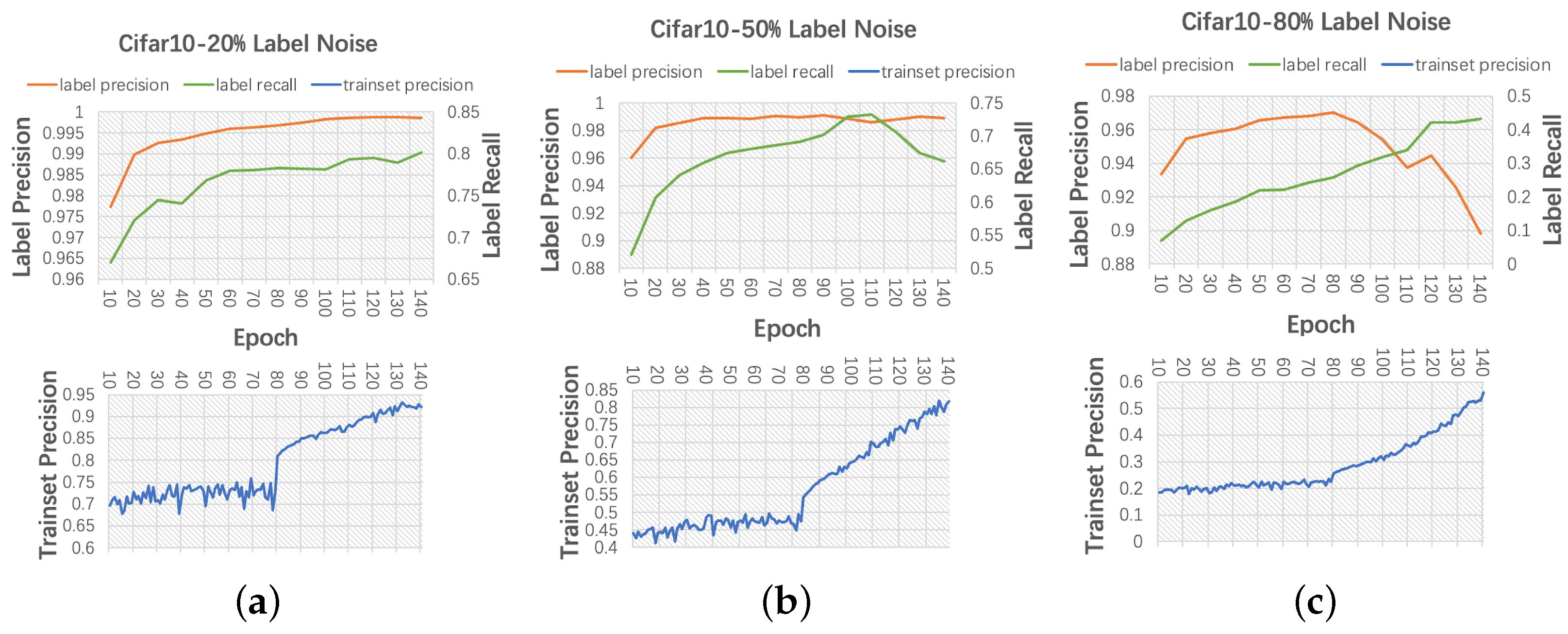
The performance of loss modeling methods in the literature is very sensitive to the choice of warmup epoch. Being too early or too late to end the warmup stage will cause either insufficient learning or over-fitting to noisy labels. As is shown in Figure 4, our method is relatively nonsensitive to the choice of warmup epoch. Under the setting of 20% and 50% noise rate, the precision of labels produced by FGCM keeps at a high point even when the model begins to be over-fitted. When the noise rate is extremely high (e.g., 80%) the precision of labels produced by FGCM slowly decreases.

4.3.2. Ablation Study on Cluster Number

Table 7 and Table 8 illustrate the precision and recall of filtered labels obtained using FGCM with different clustering numbers under different noise types and rates on CIFAR-10. For ANNO-GMM-2, we cluster samples into two categories only using the confidence of annotation label, which is the common practice adopted by previous methods [9,19]. The set with higher confidence is chosen. For FGCM-GMM-3, we cluster samples into three categories and use the set with highest sum of confidence (i.e., CS) as well as the set with biggest difference between confidence of annotation and pseudo label (i.e., NS); For FGCM-GMM-4, we cluster samples into four categories, filtering CS, NS, and CH. The results show that by clustering samples into five categories, we can achieve the highest precision of filtered labels on all the settings while the recall is still acceptable. The comparison between ANNO-GMM-2 and FGCM-GMM-5 demonstrates the effectiveness of our proposed fine-grained confidence modeling, since FGCM can achieve higher precision than ANNO-GMM-2 while the recall is far higher than that of ANNO-GMM-2. Notably, though the label precision of ANNO-GMM-2 achieves 99.79% under 40% asymmetric noise, the clean set only consists of samples from five classes while all the samples from the other five classes are in the noisy set.

4.3.3. Ablation Study on Clustering Methods

The last two rows in Table 7 and Table 8 perform a comparison between different clustering methods in FGCM. In FGCM-KMEANS-5, we use Kmeans, one of the most popular clustering algorithms, to cluster samples into five clusters based on the joint confidence scores with the maximum number of iterations and relative tolerance set to 2000 and 0.0001, respectively.
As stated in Table 7 and Table 8, GMM outperforms Kmeans. The accuracy of labels produced by GMM is higher than Kmeans especially under high noise ratios while the recall of labels is comparable. GMM is more flexible in the sharpness of distribution and more robust to outliers compared with Kmeans. Therefore, we employ GMM in this paper.

4.4. Training Time Analysis

In this section, we compare the training time of FGCM on CIFAR-10 with 50% symmetrical noise with previous methods. The results are listed in Table 9. We use a single Nvidia Tesla V100 GPU to train all the models. Co-teaching+ is the fastest but the trained performance of other methods is much higher than Co-teaching+. The training time of FGCM is slightly longer than DivideMix yet both of FGCM and DivideMix are much faster than Sel-CL+.

5. Conclusions and Future Work

In this paper, in order to train deep neural networks robustly on noisily labeled datasets by recalling more reusable training samples, we propose to categorize training samples into five kinds (i.e., Clean Simple (CS), Noisy Simple (NS), Clean Hard (CH), Noisy Hard with Relevant annotations (NHR), and Noisy Hard with Irrelevant lables (NHI)). Then, we find there are significant differences among the confidence trends of samples from the five kinds during the training process. Thus, we propose a simple yet effective framework for noisy label learning called Fine-Grained Confidence Modeling (FGCM) where samples in the training set are categorized into fine-grained categories based on the difficulty experienced by DNN models when learning the samples and label correctness.
In every epoch after a warmup process, FGCM clusters training samples into the five fine-grained categories by fitting a five-component Gaussian Mixture Model on the prediction confidence of both annotation labels and the maximum repeating pseudo labels. Then, the generated clusters are refined using their prior assumptions (e.g., annotation labels and the maximum repeating pseudo labels of NS samples should be different). Finally, a new training set with high label accuracy can be obtained by screening out instances from NHR and NHI whose labels are ambiguous, rectifying the labels of NS samples with their maximum repeating pseudo labels. By iteratively repeating the process, FGCM can gradually recall more reusable training samples from NHR and NHI. Moreover, semi-training is employed with samples from NHR and NHI treated as unlabeled data. In this way, FGCM can maximize the use of supervised labels and training samples, meanwhile preventing the model from over-fitting to noisy labels. Extensive experiments on CIFAR-10, CIFAR-100, clothing1M and Webvision demonstrate the effectiveness of FGCM.
Limitations Despite FGCM significantly outperforming previous methods, the performance will downgrade on noisy datasets with class imbalance issues, which is common in real-world datasets. The confidence of training samples will be influenced by the long-tailed distribution between different classes, making it more difficult to distinguish clean samples. Furthermore, this is one of the reasons why current noisy label learning methods struggle to achieve better performance on real-world datasets such as Clothing1M and Webvision.
Future Works Our future works will focus on three aspects: (1) The robust training of DNNs on noisily labeled imbalance datasets. (2) The training time costed by existing methods is still high especially on large scale datasets. More efficient algorithms should be developed. (3) Currently, most works on noisy label learning are focused on the task of image classification. In future, techniques of noisy label learning may extend to other visual tasks [46] or other modalities such as natural language processing [47].

Author Contributions

Conceptualization, S.Y. and X.T.; methodology, S.Y.; validation, S.Y., X.T. and R.J.; formal analysis, S.Y. and R.J.; writing—original draft preparation, S.Y.; writing—review and editing, X.T., R.J. and Y.C.; supervision, Y.C. All authors have read and agreed to the published version of the manuscript.

Funding

This work is supported by National Natural Science Foundation of China under Grant 31627802 and the Fundamental Research Funds for the Central Universities.

Institutional Review Board Statement

Not applicable.

Informed Consent Statement

Not applicable.

Data Availability Statement

The data used in this work included, i.e., CIFAR-10, CIFAR-100, Clothing1M and WebVision image sets, are openly available.

Conflicts of Interest

The authors declare no conflict of interest.

References

  1. Arpit, D.; Jastrzebski, S.; Ballas, N.; Krueger, D.; Bengio, E.; Kanwal, M.S. A closer look at memorization in deep networks. In Proceedings of the International Conference on Machine Learning, Sydney, Australia, 7–9 August 2017. [Google Scholar]
  2. Toneva, M.; Sordoni, A.; des Combes, R.T.; Trischler, A.; Bengio, Y.; Gordon, G. An empirical study of example forgetting during deep neural network learning. In Proceedings of the International Conference on Learning Representations, New Orleans, LA, USA, 6–9 May 2019. [Google Scholar]
  3. Zhang, C.; Recht, B.; Bengio, S.; Hardt, M.; Vinyals, O. Understanding deep learning requires rethinking generalization. In Proceedings of the International Conference on Learning Representations, Toulon, France, 24–26 April 2017. [Google Scholar]
  4. Krizhevsky, A.; Sutskever, I.; Hinton, G.E. Imagenet classification with deep convolutional neural networks. CACM 2017, 6, 84–90. [Google Scholar] [CrossRef] [Green Version]
  5. Redmon, J.; Divvala, S.; Girshick, R.; Farhadi, A. You only look once: Unified, real-time object detection. In Proceedings of the IEEE Conference on Computer Vision and Pattern Recognition, Las Vegas, NV, USA, 26–30 June 2016. [Google Scholar]
  6. Tanaka, D.; Ikami, D.; Yamasaki, T.; Aizawa, K. Joint optimization framework for learning with noisy labels. In Proceedings of the IEEE Conference on Computer Vision and Pattern Recognition, Salt Lake City, UT, USA, 18–22 June 2018. [Google Scholar]
  7. Liu, T.; Tao, D. Classification with Noisy Labels by Importance Reweighting. IEEE Trans. PAMI 2016, 38, 447–461. [Google Scholar] [CrossRef] [PubMed] [Green Version]
  8. Arazo, E.; Ortego, D.; Albert, P.; O’Connor, N.E.; McGuinness, K. Unsupervised label noise modeling and loss correction. In Proceedings of the International Conference on Machine Learning, Long Beach, CA, USA, 9–15 June 2019. [Google Scholar]
  9. Zhang, Z.; Zhang, H.; Arik, S.O.; Lee, H.; Pfister, T. Distilling effective supervision from severe label noise. In Proceedings of the IEEE Conference on Computer Vision and Pattern Recognition, Virtual, 14–19 June 2020. [Google Scholar]
  10. Gu, N.; Fan, M.; Meng, D. Robust Semi-Supervised Classification for Noisy Labels Based on Self-Paced Learning. IEEE SPL 2016, 23, 1806–1810. [Google Scholar] [CrossRef]
  11. Yao, J.; Wang, J.; Tsang, I.; Zhang, Y.; Sun, J.; Zhang, C.; Zhang, R. Deep Learning from Noisy Image Labels with Quality Embedding. IEEE Trans. IP 2019, 28, 1909–1922. [Google Scholar] [CrossRef] [PubMed] [Green Version]
  12. Li, S.; Xia, X.; Ge, S.; Liu, T. Selective-Supervised Contrastive Learning with Noisy Labels. In Proceedings of the IEEE Conference on Computer Vision and Pattern Recognition, New Orleans, LA, USA, 21–24 June 2022. [Google Scholar]
  13. Yi, R.; Huang, Y. TC-Net: Detecting Noisy Labels via Transform Consistency. IEEE Trans. Multimed. 2021, 24, 4328–4341. [Google Scholar] [CrossRef]
  14. Bernhardt, M.; Castro, D.C.; Tanno, R.; Schwaighofer, A.; Tezcan, K.C.; Monteiro, M.; Bannur, S.; Lungren, M.P.; Nori, A.; Glocker, B.; et al. Active label cleaning for improved dataset quality under resource constraints. Nat. Commun. 2022, 13, 1161. [Google Scholar] [CrossRef] [PubMed]
  15. Liu, S.; Niles-Weed, J.; Razavian, N.; Fernandez-Granda, C. Early-learning regularization prevents memorization of noisy labels. In Proceedings of the Conference on Neural Information Processing Systems, Virtual, 6–12 December 2020. [Google Scholar]
  16. Jiang, L.; Zhou, Z.; Leung, T.; Li, L.; Li, F.-F. MentorNet: Learning data-driven curriculum for very deep neural networks on corrupted labels. In Proceedings of the International Conference on Machine Learning, Stockholm, Sweden, 10–15 July 2018. [Google Scholar]
  17. Han, B.; Yao, Q.; Yu, X.; Niu, G.; Xu, M.; Hu, W. Co-teaching: Robust training of deep neural networks with extremely noisy labels. In Proceedings of the Conference on Neural Information Processing Systems, Montreal, QC, Canada, 2–8 December 2018. [Google Scholar]
  18. Yu, X.; Han, B.; Yao, J.; Niu, G.; Tsang, I.W.; Sugiyama, M. How does disagreement help generalization against label corruption? In Proceedings of the International Conference on Machine Learning, Long Beach, CA, USA, 9–15 June 2019. [Google Scholar]
  19. Li, J.; Socher, R.; Hoi, S. Dividemix: Learning with noisy labels as semi-supervised learning. In Proceedings of the International Conference on Learning Representations, Virtual, 26–30 April 2020. [Google Scholar]
  20. Patrini, G.; Rozza, A.; Menon, A.K.; Nock, R.; Qu, L. Making deep neural networks robust to label noise: A loss correction approach. In Proceedings of the IEEE Conference on Computer Vision and Pattern Recognition, Honolulu, HI, USA, 22–25 July 2017. [Google Scholar]
  21. Chen, X.; Gupta, A. Webly supervised learning of convolutional networks. In Proceedings of the International Conference on Computer Vision, Santiago, Chile, 13–16 December 2015. [Google Scholar]
  22. Xiao, T.; Xia, T.; Yang, Y.; Huang, C.; Wang, X. Learning from massive noisy labeled data for image classification. In Proceedings of the IEEE Conference on Computer Vision and Pattern Recognition, Boston, MA, USA, 8–10 June 2015. [Google Scholar]
  23. Ghosh, A.; Kumar, H.; Sastry, P. Robust loss functions under label noise for deep neural networks. In Proceedings of the AAAI Conference on Artificial Intelligence, San Francisco, CA, USA, 4–9 February 2017. [Google Scholar]
  24. Zhang, Z.; Sabuncu, M. Generalized cross entropy loss for training deep neural networks with noisy labels. In Proceedings of the Conference on Neural Information Processing Systems, Montreal, QC, Canada, 2–8 December 2018. [Google Scholar]
  25. Wang, Y.; Ma, X.; Chen, Z.; Luo, Y.; Yi, J.; Bailey, J. Symmetric cross entropy for robust learning with noisy labels. In Proceedings of the IEEE/CVF International Conference on Computer Vision, Seoul, Korea, 27–31 October 2019. [Google Scholar]
  26. Chen, P.; Liao, B.B.; Chen, G.; Zhang, S. Understanding and utilizing deep neural networks trained with noisy labels. In Proceedings of the International Conference on Machine Learning, Long Beach, CA, USA, 9–15 June 2019. [Google Scholar]
  27. Nguyen, D.T.; Mummadi, C.K.; Ngo, T.P.N.; Nguyen, T.H.P.; Beggel, L.; Brox, T. SELF: Learning to filter noisy labels with self-ensembling. In Proceedings of the International Conference on Learning Representations, Virtual, 26–30 April 2020. [Google Scholar]
  28. Ortego, D.; Arazo, E.; Albert, P.; O’Connor, N.E. Multi-objective interpolation training for robustness to label noise. In Proceedings of the IEEE Conference on Computer Vision and Pattern Recognition, Virtual, 20–25 June 2021. [Google Scholar]
  29. Permuter, H.; Francos, J.; Jermyn, I. A study of gaussian mixture models of color and texture features for image classification and segmentation. Pattern Recognit. 2006, 39, 695–706. [Google Scholar] [CrossRef]
  30. Dempster, A.P.; Laird, N.M.; Rubin, D.B. Maximum likelihood from incomplete data via the EM algorithm. R. Stat. Soc. 1977, 39, 1–38. [Google Scholar]
  31. Sohn, K.; Berthelot, D.; Carlini, N.; Zhang, Z.; Zhang, H.; Raffel, C. Fixmatch: Simplifying semi-supervised learning with consistency and confidence. In Proceedings of the Conference on Neural Information Processing Systems, Virtual, 6–12 December 2020. [Google Scholar]
  32. Krizhevsky, A.; Nair, V.; Hinton, G. CIFAR-10 CIFAR-100; Canadian Institute for Advanced Research: Toronto, ON, Canada, 2021. [Google Scholar]
  33. Li, W.; Wang, L.; Li, W.; Agustsson, E.; Gool, L.V. Webvision database: Visual learning and understanding from web data. arXiv 2017, arXiv:1708.02862. [Google Scholar]
  34. Song, H.; Kim, M.; Park, D.; Lee, J. Prestopping: How does early stopping help generalization against label noise? In Proceedings of the International Conference on Machine Learning, Long Beach, CA, USA, 9–15 June 2019. [Google Scholar]
  35. He, K.; Zhang, X.; Ren, S.; Sun, J. Identity mappings in deep residual networks. In Proceedings of the European Conference on Computer Vision, Amsterdam, The Netherlands, 8–16 October 2016. [Google Scholar]
  36. He, K.; Zhang, X.; Ren, S.; Sun, J. Deep residual learning for image recognition. In Proceedings of the IEEE Conference on Computer Vision and Pattern Recognition, Las Vegas, NV, USA, 26–30 June 2016. [Google Scholar]
  37. Szegedy, C.; Ioffe, S.; Vanhoucke, V.; Alemi, A. Inception-v4, inception-resnet and the impact of residual connections on learning. In Proceedings of the AAAI Conference on Artificial Intelligence, San Francisco, CA, USA, 4–9 February 2017. [Google Scholar]
  38. Yi, K.; Wu, J. Probabilistic end-to-end noise correction for learning with noisy labels. In Proceedings of the IEEE Conference on Computer Vision and Pattern Recognition, Long Beach, CA, USA, 16–20 June 2019. [Google Scholar]
  39. Kim, T.; Ko, J.; Choi, J.; Yun, S.Y. Fine samples for learning with noisy labels. In Proceedings of the Conference on Neural Information Processing Systems, Virtual, 7–10 December 2021. [Google Scholar]
  40. Li, J.; Wong, Y.; Zhao, Q.; Kankanhalli, M.S. Learning to learn from noisy labeled data. In Proceedings of the IEEE Conference on Computer Vision and Pattern Recognition, Long Beach, CA, USA, 16–20 June 2019. [Google Scholar]
  41. Wu, Y.; Shu, J.; Xie, Q.; Zhao, Q.; Meng, D. Learn To Purify Noisy Labels via Meta Soft Label Corrector. In Proceedings of the AAAI Conference on Artificial Intelligence, Virtual, 2–9 February 2021. [Google Scholar]
  42. Zhang, W.; Wang, Y.; Qiao, Y. Metacleaner: Learning to hallucinate clean representations for noisy-labeled visual recognition. In Proceedings of the IEEE Conference on Computer Vision and Pattern Recognition, Long Beach, CA, USA, 16–20 June 2019. [Google Scholar]
  43. Malach, E.; Shalev-Shwartz, S. Decoupling “when to update” from “how to update”. In Proceedings of the Conference on Neural Information Processing Systems, Long Beach, CA, USA, 4–7 December 2017. [Google Scholar]
  44. Ma, X.; Wang, Y.; Houle, M.; Zhou, S.; Erfani, S.; Xia, S.; Wijewickrema, S.; Bailey, J. Dimensionality-driven learning with noisy labels. In Proceedings of the International Conference on Machine Learning, Stockholm, Sweden, 10–15 July 2018. [Google Scholar]
  45. Li, J.; Xiong, C.; Hoi, S. Learning from noisy data with robust representation learning. In Proceedings of the International Conference on Computer Vision, Virtual, 11–17 October 2021. [Google Scholar]
  46. Yang, M.; Huang, Z.; Hu, P.; Li, T.; Lv, J.; Peng, X. Learning with Twin Noisy Labels for Visible-Infrared Person Re-Identification. In Proceedings of the IEEE Conference on Computer Vision and Pattern Recognition, New Orleans, LA, USA, 21–24 June 2022. [Google Scholar]
  47. Wang, Y.; Baldwin, T.; Verspoor, K. Noisy Label Regularisation for Textual Regression. In Proceedings of the International Conference on Computational Linguistics, Gyeongju, Korea, 10–12 October 2022. [Google Scholar]
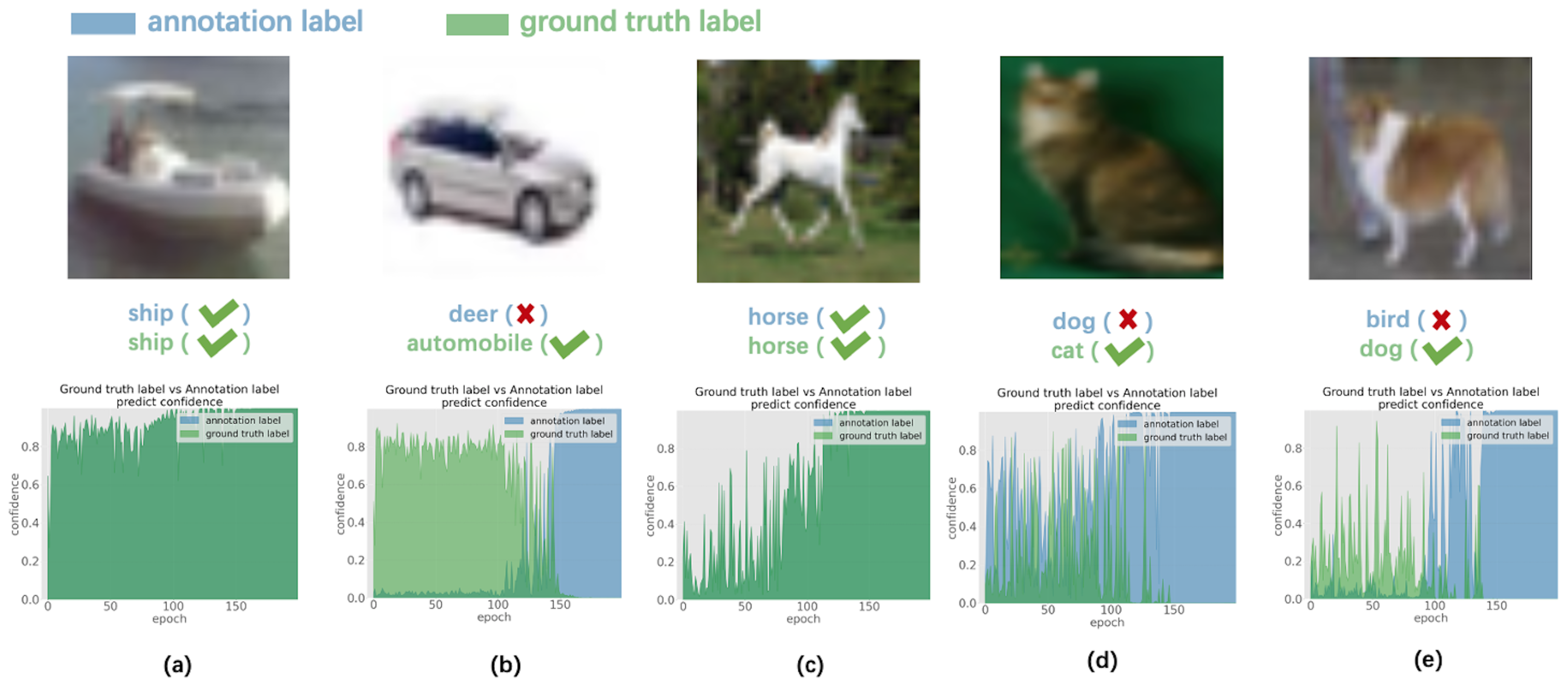
Figure 1. Typical examples of images in the training set and corresponding confidence score trends for different kinds of samples on CIFAR-10 with 20% symmetrical noise. The words in blue below each image are their annotation labels which might be wrong, while the green words are the ground truth labels. The crosses or ticks in brackets indicate the rightness of corresponding labels. We train a PreAct-18 resnet using SGD with a momentum of 0.9, a weight decay of 0.0005, and a batch size of 128. The initial learning rate is set to 0.06 and reduced to 0.006 in the 80th epoch. The blue and green curves represent the trends of confidence scores for annotation labels and ground truth labels during the training process, respectively. (a) Clean Simple samples (CS) (i.e., highly distinguishable instances with correct annotations). (b) Noisy Simple samples (NS) (i.e., mislabeled samples with easily identifiable features). (c) Clean Hard samples (CH). (d) Noisy Hard samples with Relevant annotations (NHR). (e) Noisy Hard samples with Irrelevant labels (NHI).
Applsci 12 11406 g001
Figure 2. Sample clusters generated by FGCM. (a) is generated using confidence score of ground truth labels and annotation labels. (b) is generated using confidence score of maximum repeating pseudo labels and annotation labels.
Applsci 12 11406 g002
Figure 3. Examples of rectified labels by FGCM in Clothing1M and WebVision datasets. Red labels denote original annotations which are obviously wrong. Green labels denote rectified labels produced by FGCM which are obviously correct.
Applsci 12 11406 g003
Figure 4. Precision and recall of labels produced by FGCM under different noise rates on CIFAR-10 dataset vs. the precision on trainset during training. The orange curves represent the precision of labels of the labeled trainset produced by FGCM. The green curves show the recall of the labeled trainset produced by FGCM. The blue curves illustrate the precision of models on the original trainset. (a) Results on CIFAR-10 with 20% symmetric label noise. (b) Results on CIFAR-10 with 50% symmetric label noise. (c) Results on CIFAR-10 with 80% symmetric label noise.
Applsci 12 11406 g004
Table 1. Summary of literature reviewed according to the category of methods.
CategoryMethods
Noise transition matrixFcorr [20], Webly learning [21], Probabilistic noise modeling [22]
Robust Loss FunctionRobust MAE [23], Generalized Cross Entropy [24], Symmetric Cross Entropy [25]
Sample SelectionMentorNet [16], Co-teaching [17], Co-teaching+ [18], Iterative-CV [26]
Hybrid MethodsSELF [27], Mcorr [8], DivideMix [19], MOIT+ [28], Sel-CL+ [12]
Table 4. Performance comparison with state-of-the-art methods on clothing1M.
MethodTCNet [13]Meta-Cleaner [42]ELRFINEMSLCDivide-Mix+ELR+FGCM
Accuracy71.1572.5072.8772.9174.0274.7674.8174.91
Table 5. Performance comparison with state-of-the-art methods on WebVision validation set and the ImageNet ILSVRC12 validation set. Results for baseline methods are copied from [12,15,19].
MethodWebVisionILSVRC12
Top1Top5Top1Top5
Fcorr [20]61.1582.6857.3682.36
Decoupling [43]62.5484.7458.2682.26
D2L [44]62.6884.0057.8081.36
MentorNet [16]63.0081.4057.8079.92
Co-teaching [17]63.5885.2061.4884.70
Iterative-CV [26]65.2485.3461.6084.98
DivideMix+ [19]77.3291.6475.2090.84
ELR [15]76.2691.2668.7187.84
ELR+ [15]77.7891.6870.2989.76
ProtoMix [45]76.391.573.391.2
FGCM77.8491.7674.5690.24
Table 6. Ablation Study results on CIFAR-10 with two different noise rates.
DatasetCIFAR-10
Method Noise RatesSym 20%Sym 80%
FGCM (CS + NS + CH + NHI + NHR + cluster refinement)95.694.1
FGCM (CS + NS + CH + NHI + NHR95.293.6
FGCM (CS + CH + NHI + NHR)94.593.0
FGCM (CS + NS + CH)93.876.9
FGCM w/o fine-grained sample categorization88.2550.0
Cross Entropy86.862.9
Table 7. Precision of obtained labels using different clustering methods and cluster numbers on CIFAR-10 with different type and ratios of noise. ANNO-GMM-2 denotes experiment that only uses the confidence of annotation label to divide samples into two categories.
Methods-Cluster NumSym 20%Sym 50%Sym 80%Asym 40%
ANNO-GMM-299.7097.9496.7399.79
FGCM-GMM-397.6797.2096.1995.94
FGCM-GMM-499.1097.4295.4095.40
FGCM-KMEANS-599.7598.3395.9395.13
FGCM-GMM-599.7599.0297.2397.04
Table 8. Recall of obtained labels using different clustering methods and cluster numbers on CIFAR-10 with different type and ratios of noise. ANNO-GMM-2 denotes experiment that only uses the confidence of annotation label to divide samples into two categories.
Methods-Cluster NumSym 20%Sym 50%Sym 80%Asym 40%
ANNO-GMM-277.0552.0916.4441.39
FGCM-GMM-379.6873.2835.8458.72
FGCM-GMM-483.8071.0432.5763.20
FGCM-KMEANS-577.5666.4033.7860.83
FGCM-GMM-579.3571.4229.5760.59
Table 9. Comparison of total Training Time on CIFAR-10 with 50% symmetrical label noise, using a single Nvidia Telsa V100 GPU.
Co-Teaching+PcorrMeta-LearningDivideMixSel-CL+FGCM
4.3 h6.0 h8.6 h5.2 h7.2 h5.4 h
Publisher’s Note: MDPI stays neutral with regard to jurisdictional claims in published maps and institutional affiliations.