Granular Description of Uncertain Data for Classification Rules in Three-Way Decision

Abstract

Considering that data quality and model confidence bring threats to the confidence of decision-making, a three-way decision with uncertain data description is more meaningful in system analyses. In this paper, an advanced method for forming classification rules in three-way decisions is proposed. This method firstly constructs information granules for describing uncertain data in decision-making; meanwhile, information entropy is introduced in Granular Computing (GrC) to realize a better uncertainty description. Then, based on the constructed uncertainty descriptors, fuzzy rules are formed aiming at the common decision-making processes, namely classification problems. Finally, experiments on both synthetic and publicly available data are implemented. Discussions on numerical results validate the feasibility of the proposed method for forming three-way classification rules. Moreover, classification rules with consideration of uncertain data are demonstrated to be better performed than traditional methods with an improvement of 1.35–4.26% in decision-making processes.

1. Introduction

In the current information era, decision-making in industrial systems becomes more and more reliable to data, that is to say, a confident decision relies much on the confidence of data [1]. However, due to various reasons in the real-world context, it is commonly found that collected data contains noise, faults, anomalies, mismatches or other problematical samples [2]. When considering data with these kinds of issues in data-driven modeling, the learned systems would not be justified for decision-making analysis. On the other hand, the basic decision in system analysis is commonly known in a binary way. A complex decision-making process can be regarded as the combination of several binary decisions, e.g., the multi-classes classification [3]. However, the decision results are not always confident for customers due to some data quality problems, such as adversarial data, boundary data, etc. [4]. For example, in a binary classification problem, there could be a situation where the prediction probability of two classes is very close, e.g., 0.49 vs. 0.51. In this case, the general two standard alternatives are not suitable, and they should be included with a warning for the third option, e.g., unclear scenarios in autonomous driving decision systems [5]. Therefore, further investigation from humans is required to guarantee confidence in the final decisions. In a word, considering data quality, a three-way decision would be more meaningful and reliable than a two-way decision in the decision-making of real-world industrial systems.

The essence of the three-way decision process is actually extending two-valued logic to three-valued logic, namely considering acceptance, rejection and uncertainty in decisions [6]. This logic is attractive for developing multiple-valued logic models; for example, some interesting applications related to machine learning and software programming [7,8]. To realize this kind of decision mechanism, fuzzy and rough sets are the two most common options in three-way decisions [9] in the literature review. For example, three-valued logics were described by rough sets directly as well as their extensions in [10]. In [11], an advanced three-way decision model was developed based on the combination of rough sets and game theory. This method proposed to set up optimal parameters to construct probabilistic rough sets for describing the related logic in the three-way decision. Furthermore, the game theory was introduced in the formulation of an objective function aiming to minimize the uncertainty of the probabilistic rough sets in the three-way decision; then, the determined parameters were used for the distinction of certain and uncertain logics [12]. Moreover, the shadow set is a kind of development on fuzzy sets which can be used to generalize the decision-making into a three-valued determination process. For instance, in [13] they were effectively leveraged to support the three-way decision. Moreover, some advanced three-way decision methods were modeled based on the methodology of Granular Computing (GrC) [14,15], which can make use of different granularity to describe the uncertainty in three-valued logics, so they can have more flexibility than generic fuzzy-sets- or rough-sets-based methods. In [16], a granular method was proposed for the problem of record linkage which is regarded as a three-way decision.

On the other hand, by summarizing three-way methods in the literature, it is found that uncertainty is the key factor affecting the final performance of decision-making. If more and deeper investigation on uncertainty itself is available, the negative influence of uncertainty in three-way decisions can be reduced. Therefore, describing the uncertain data along with certain data is a necessary technique in uncertainty investigation for three-way decisions. According to existing studies reported in [17], uncertainty is generally taken from the negative parts of the two-way decision. For example, in a two-classes (denoted as ClassA and ClassB) classification problem, the uncertain region is formed by data points of both not-ClassA and not-ClassB, namely the negative regions of ClassA and ClassB. To describe these uncertainty regions, fuzzy or rough sets are applied in three-way decision methods. Then, probability and fuzzy membership are utilized as two common indicators expressing uncertainty in the final decision-making. Compared with fuzzy-/rough-set-based methods, granules via GrC seem more natural to describe the uncertainty regions [18], especially in decision-making with multiple-level mechanisms [19]. For example, in a classification problem, the generic two-way decision requires finding an optimal threshold on decision indicators to divide the output space into two regions representing two classes. For three-way decisions, the indicator value of uncertain data would lie around the threshold of two-way decisions, e.g., 0.5 of probability or membership. By making use of GrC, we can easily extend the threshold to a granular interval for three regions’ descriptions. By optimizing this granular interval to have a high coverage of uncertain data, the performance of three-way decisions would be improved.

According to the above descriptions, in this paper, we develop a granular method for three-way decisions. Firstly, to enhance the data description ability, this paper proposed utilizing information granules (IGs) instead of fuzzy or rough sets [20] in the description of certain and uncertain data in data space directly. Meanwhile, to express the uncertainty of data, information entropy is introduced in the process of GrC to construct granules with better information description ability. Then, based on these constructed granular descriptors, fuzzy rules are formed and used to guide the final three-way decision-making in the following way. For example, a rule via the uncertain descriptor is formed to distinguish uncertain data for “clerical investigation”. Moreover, certain data is also described by some granules and recognized into different classes via the formed rules in a generic two-way decision process. With the help of the proposed method, three contributions are obtained in this paper.

(1)

A three-way decision method based on granular classification rules is proposed for decision-making in this paper. By making use of granules’ advantages on data description [21,22], this method combines GrC and FCM (Fuzzy C-Means) [23] to construct uncertain data descriptors and to guide the formation of classification rules in three-way decision-making. As we know, FCM is a commonly used algorithm for data clustering. Here, it is a novelty developed for decision-making with the help of granules for data description and validated feasible to solve the uncertainty investigation in classification problems;

(2)

Three-way decisions in various scenarios are studied via the proposed method. For example, three-way decisions in one-dimensional and high-dimensional data spaces are separately discussed, including the granular descriptors construction, rules formation and the final decision-making process. All implementations are demonstrated feasible and effective through experiments on synthetic and public data;

(3)

Good performances are verified in uncertainty data descriptions and three-way decisions. In this paper, firstly, several useful evaluation metrics are developed for uncertainty description. Then, both synthetic data and publicly available data are applied to evaluate the performance of the proposed three-way decision method. By considering different parameters in constructing uncertainty granules, the performance of decision-making in classification problems is discussed. The feasibility and effectiveness of the proposed method are validly demonstrated.

Besides the introduction part, Section 2 describes the problem of uncertain data in the decision-making process of classification problems. Section 3 describes the processes of how to construct information granules for describing uncertainty. Section 4 provides the definitions of some useful evaluation metrics. Section 5 presents the experimental results on both synthetic data and publicly available data based on the proposed three-way decision with granular uncertainty descriptors. Finally, Section 6 concludes the work in this paper.

2. Problem Formulation

2.1. Overview of Uncertain Data

In decision-making, data types could be divided into three categories, such as labeled data, unlabeled data and semi-labeled data, as shown in Figure 1. According to these data types, a general decision-making problem, a classification problem, could be divided into three types: supervised classification, unsupervised classification and semi-classification [24]. In Figure 1a, the labeled data is assumed as {(x,y)|x∈Rⁿ}, where x is the input data and y is the label variable. Its classification rules are constructed by commonly used supervised classifiers, e.g., support vector machine (SVM), decision trees (DT), neural networks (NN) and so on [25,26]. Due to taking the label variable y as a reference in training, these classifiers can achieve good performance on most of the data. However, misclassification usually happens on the boundary of two classes, as seen in Figure 1a. In Figure 1b, the unlabeled data contains only inputs, expressed as {x|x∈Rⁿ}. Due to the lack of transcendental categories information, its classification rules are constructed by unsupervised classifiers, namely clustering algorithms for determining classes. FCM clustering is a typical unsupervised classification algorithm used in the literature [27]. It is seen from Figure 1b that data points in the overlap of two clusters are difficult to classify. In Figure 1c, the given dataset is divided into two parts, the labeled part {(x₁,y₁), (x₂,y₂), …, (x_r,y_r)} and the unlabeled part {x_r+1, x_r+2, …, x_N}, where N and r are the number of data points in the whole dataset and labeled part, respectively. Usually, its classification rules are constructed through a two-phase process. Firstly, a classifier is trained by the labeled data. Then, the unlabeled data points are labeled based on the constructed classifier. It is seen that there are two uncertain regions. One is the boundary of two classes in the labeled part, the other one is the overlap in the unlabeled part.

Through the discussion of Figure 1, it is seen that, with respect to no matter which type of classification, there exist uncertain data points affecting the accuracy of classification rules, e.g., in misclassification regions or overlap regions. To improve the efficiency and effectiveness of classification, this is a good way to extract these data points as an uncertain region for manual recognition and “clerical review”. Then, with the description of uncertain regions, we can construct better classification rules for high-performance classification.

2.2. Data Classification via FCM

(1)

Unlabeled data

To describe the uncertainty of classification, fuzzy classifiers are superior to certain classifiers. Therefore, we propose to apply FCM in classification. Since FCM is a typical unsupervised classification algorithm in pattern recognition, it is primarily used for unlabeled datasets. Assuming a dataset {x_k|x_k∈Rⁿ, k = 1, 2, …, N} with c categories, it can be partitioned by FCM via the membership matrix U and c prototypes. The definition of the membership matrix is expressed in the following formula:

$$\mathit{U}={\left[u_{ik}\right]}_{c\times N}; u_{ik}=\frac{1}{{\displaystyle \sum _{j=1}^c{\left(\frac{‖{\mathit{x}}_k-{\mathit{v}}_i‖}{‖{\mathit{x}}_k-{\mathit{v}}_j‖}\right)}^{2/(m-1)}}}$$

(1)

where x_k is a point in the given dataset; v_i is ith prototype; u_ik is the membership to the ith cluster; m is a parameter controlling the fuzzification degree. The ith prototype, namely the cluster center of the ith fuzzy cluster, can be calculated as seen below.

$${\mathit{v}}_i={\displaystyle \sum _{k=1}^N{u}_{ik}^m{\mathit{x}}_k}/{\displaystyle \sum _{k=1}^N{u}_{ik}^m}$$

(2)

Combining Formulas (1) and (2), the objective function ${\displaystyle \sum _{k=1}^N{\displaystyle \sum _{j=1}^c{u}_{ik}^m{‖{\mathit{x}}_k-{\mathit{v}}_i‖}^2}}$ can be minimized via iterative optimization. It is seen that the values of u_ik satisfy 0 ≤ u_ik ≤ 1 and ${\displaystyle \sum _{i=1}^c{u}_{ik}}=1$. Through the partition matrix U, unsupervised classification rules are constructed by memberships.

(2)

Labeled data

For labeled datasets, their category labels are given in advance. By utilizing FCM clustering on data {x_k}, new labels are generated according to the above processes, which may be in conflict with given labels {y_k}. To copy labeled data with FCM, we modified its objective function as seen below.

$${\displaystyle \sum _{k=1}^N{\displaystyle \sum _{i=1}^c{u}_{ik}^m{‖{\mathit{x}}_k-{\mathit{v}}_i‖}^2}}+C{\displaystyle \sum _{k=1}^N{\displaystyle \sum _{i=1}^c{‖y_k-y_{v_i}‖}^2}}$$

(3)

where y_k is the actual label of data point x_k; y_vi is the label of prototype v_i; C is a penalty factor. The new objective function has two parts. The first part is the general objective function for clustering unlabeled data in FCM. The second part is defined by only the label variable y_k; its purpose is to group data points with the same labels into a cluster. The value of C is determined according to application requirements. For example, when C = 0, the formula (3) degenerates for the generic FCM clustering on unlabeled data. When C = 1, we could regard the process as FCM clustering on dataset {(x_k, y_k)|k = 1, 2, …, N}. When C is extremely large, the influence of the first part of (3) will be ignored, then (3) degenerates as the objective function for supervised classification. Usually, to apply FCM clustering more appropriately on labeled data, a suitable value of C is selected for considering the penalty in misclassification on the label variable.

(3)

Semi-labeled data

For semi-labeled datasets, there are two ways to apply FCM in classification. The first way is mentioned above, which processes the labeled part first and classifies the unlabeled part second. The second way is to apply the FCM algorithm for all data points by modifying the objective function. Similar as the FCM clustering on labeled data, we can also add the penalty on the labeled part as (3) to construct the objective function.

2.3. Construction of Classification Rules

Through the above processes, the FCM algorithm can be applied to the classification of any type of dataset. The membership matrix U and category prototypes v_i are obtained for constructing classification rules. Generally, the maximum membership is used to determine a datum point’s belonging category. However, we intuitively believe that data points with a membership close to 0.5 could not be convincedly classified into any categories, e.g., the uncertain regions in Figure 1. Therefore, the proposed approach describes the uncertain region first, then constructs classification rules with consideration of both uncertain regions and the membership matrix. Assuming the uncertain region is expressed as Ω, the classification rules could be presented as seen below.

$$\left\{\begin{array}{l}Rule 1: \mathrm{IF} {\mathit{x}}_k\in \mathsf{\Omega }, \mathrm{THEN} y_k \mathrm{needs} “\mathrm{clerical} \mathrm{review}”\\ \underset{i>1}{Rule} i: \mathrm{IF} {\mathit{x}}_k\notin \mathsf{\Omega } and u_{ik}>\underset{\forall j\ne i}{u_{jk}}, \mathrm{THEN} y_k \mathrm{is} \mathrm{in} \mathrm{Class} i\end{array}\right.$$

(4)

where x_k is a tested point and y_k is the final label based on the given classification rules. Based on these rules, it is seen that when the testing data x_k belongs to an uncertain region, then “clerical review” is required to determine its final class. If not, then its belonging can be determined according to the general decision-making rules.

3. Granular Uncertainty Description

It is known from the above description that the crux of constructing high-performance classification rules is to describe the uncertain data properly. Based on the framework of data description, two factors are mainly involved, such as the prototype and size of a descriptor [28]. The prototype is usually used to locate the descriptor’s position. The size factor is used to determine the active area of the constructed descriptor. In this paper, we propose to construct an information granule via a justifiable granulating algorithm as the descriptor of an uncertain region. Then, the constructed uncertain granule will be used to determine which points are required for “clerical review” in classification, and more effective classification rules could be subsequently formed.

3.1. One-Dimensional Data with Two Categories

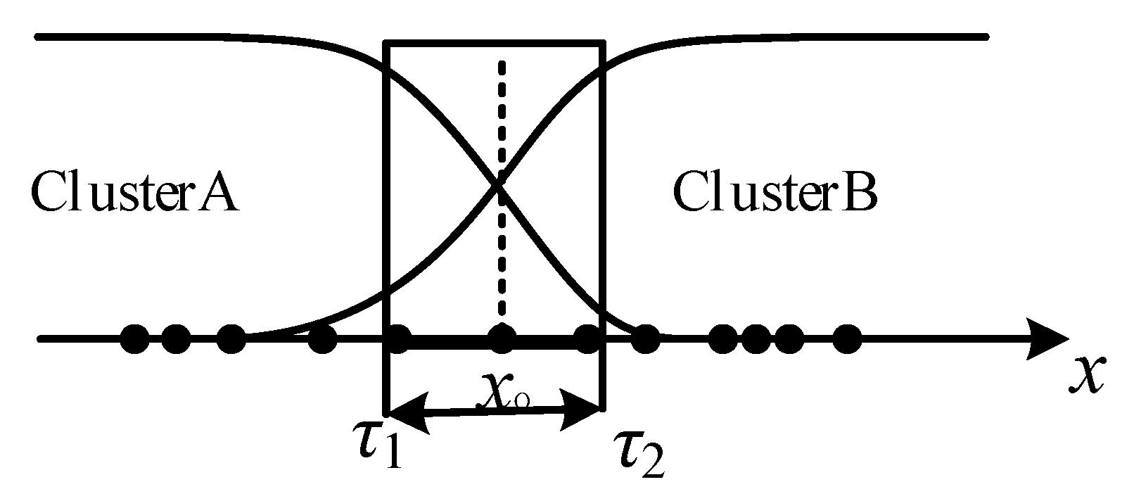
As we know, one-dimensional data with two categories is the simplest and primary data formation in pattern recognition. Assuming a one-dimensional dataset {x₁, x₂, …, x_N} uniformized into [0, 1], it is divided into two clusters (ClusterA and ClusterB) via FCM, shown in Figure 2, where uncertain data points requiring “clerical review” are included in the square region. As the above assumption, there are two parameters required in the process of granular descriptor construction, such as the prototype x_o and the size (τ₁ and τ₂) of the granule.

(1)

Selection of the prototype x_o

The function of the granular descriptor’s prototype is to locate the uncertain region so we can select the prototype as the median point having the highest uncertainty. As we know, the membership could reflect the uncertainty of data points to some extent, so they could be referred to in order to select the prototype.

First, by referring to (1) and setting the dataset’s dimension n = 1 and the number of clusters c = 2, a point’s memberships to two clusters are calculated in detail as seen below.

$$A(x)=1/{\displaystyle \sum _{i=A,B}^{}{\left(\frac{\left|x-v_{\mathrm{A}}\right|}{\left|x-v_i\right|}\right)}^2}=\frac{{\left|x-v_{\mathrm{B}}\right|}^2}{{\left|x-v_{\mathrm{A}}\right|}^2+{\left|x-v_{\mathrm{B}}\right|}^2}$$

(5)

$$B(x)=1/{\displaystyle \sum _{i=\mathrm{A},\mathrm{B}}^{}{\left(\frac{\left|x-v_{\mathrm{B}}\right|}{\left|x-v_i\right|}\right)}^2}=\frac{{\left|x-v_{\mathrm{A}}\right|}^2}{{\left|x-v_{\mathrm{A}}\right|}^2+{\left|x-v_{\mathrm{B}}\right|}^2}$$

(6)

where A(x) and B(x) are the calculation of membership with respect to (w.r.t) two clusters and v_A and v_B are the prototypes of two fuzzy clusters. Then, according to Figure 2, the median point x_o most possibly could be decided as the following criterion:

$$A(x_0)\approx B(x_0)$$

(7)

(2)

Determination of the uncertain region size

It is seen from Figure 2 that the uncertain region is determined by two parameters, namely τ₁ and τ₂. These two parameters determine the range of data points in each cluster required for “clerical review”. Therefore, with respect to one-dimensional data, the descriptor of the uncertain region around x_o is expressed by the following interval:

$$\left[x_o-{\tau }_1,x_o+{\tau }_2\right]$$

(8)

In the real-world decision-making process, we expect to obtain high accuracy with low computation overhead, so it is required to correctly classify which data points require “clerical review”. To realize these objectives, selection of the uncertain region’s size is first required to contain most of the data with high uncertainty degree. Then, this region should also guarantee high specificity of uncertain data for high-performed decision-making. To realize these requirements, the justifiable granulating algorithm [29] is applied here to realize the optimization of τ₁ and τ₂ separately.

For determining the value of τ₁, we define coverage and specificity functions first [30]. To describe the coverage of uncertain data, a function considering the data points’ uncertainty degree is defined as seen below.

$$\mathrm{cov}({\tau }_1)={\displaystyle \sum _{x_k\in [x_0-{\tau }_1, x_0]}^{}\frac{1}{2}\left\{(\max \left(h(A(x_k)),h(B(x_k))\right)+\min \left(h(A(x_k)),h(B(x_k))\right)\right\}}$$

(9)

where x_k is a data point belonging to the region [x₀ − t₁, x₀] and h(.) is denoted as an entropy function representing the uncertainty degree. To describe the uncertainty of data in the boundary of two classes, the function h(.) is required to satisfy the following conditions. Firstly, in the left region [0, 1/2], h(.) is a monotone increasing function; conversely, it is a monotone decreasing function in the region of [1/2, 1]. Secondly, it should satisfy h(0) = h(1) = 0, h(1/2) = 1. To realize these requirements, the well-known information entropy [31] function is introduced here, as

$$h(u)=-u\cdot \log (u)-(1-u)\cdot \log (1-u)$$

(10)

where u is the membership value of a given testing data point and −u∙log(u) and −(1 − u)∙log(1 − u) represent the uncertainty belonging and not-belonging to the cluster, respectively. By summing them up, the total uncertainty of a testing point is expressed as h(u).

Moreover, the specificity could be endowed with the size parameter τ₁ (0 ≤ τ₁ ≤ x₀), as seen below.

$$spe({\tau }_1)={(1-{\tau }_1)}^{\beta }$$

(11)

where β is a parameter determining the variance rate of specificity.

It is seen that the coverage function in (9) describes the total uncertainty of data points within ClusterA, which is an increasing function to τ₁. The specificity function in (11) is a decreasing function to τ₁. To optimize the information granule, both two functions are required to be at maximum. However, it is obvious these two functions are in conflict. Therefore, we define the optimization criterion by a product [32], as below.

$$Q({\tau }_1)=\mathrm{cov}({\tau }_1)\cdot spe({\tau }_1)$$

(12)

The uncertain granular interval in ClusterA could be determined by the optimal parameter τ₁, as seen below.

$${\tau }_{1,}{}_{opt}={\mathrm{argmax}}_{{\tau }_1}Q({\tau }_1)$$

(13)

where argmax implies the operator is seeking the maximum values from the given function.

For determining the value of τ₂ (x₀ ≤ τ₂ ≤ 1), the same steps are implemented. The two functions are defined as below.

$$\mathrm{cov}({\tau }_2)={\displaystyle \sum _{x_k\in [x_0, x_0+{\tau }_2]}^{}\frac{1}{2}\left\{(\max \left(h(A(x_k)),h(B(x_k))\right)+\min \left(h(A(x_k)),h(B(x_k))\right)\right\}}$$

(14)

$$spe({\tau }_2)={(1-{\tau }_2)}^{\beta }$$

(15)

Similarly, the uncertain granular interval in ClusterB could be determined by the optimal parameter τ₂ through the product ${\tau }_{2,}{}_{opt}={\mathrm{argmax}}_{{\tau }_2}Q({\tau }_2)$.

After construction of the uncertain granule, we could form classification rules according to (4). While considering the particularity of one-dimensional data, both the membership and the size of uncertain regions could be reflected by data values. Therefore, we can rewrite the classification rules as seen below.

$$\left\{\begin{array}{l}Rule 1: \mathrm{IF} x_k\in [x_0-{\tau }_1, x_0+{\tau }_2], \mathrm{THEN} y_k \mathrm{needs} “\mathrm{clerical} \mathrm{review}”;\\ Rule 2: \mathrm{IF} x_k<x_0-{\tau }_1, \mathrm{THEN} y_k{ \mathrm{is} \mathrm{in} \mathrm{Cluster}}_{\mathrm{A}};\\ Rule 3: \mathrm{IF} x_k>x_0+{\tau }_2, \mathrm{THEN} y_k{ \mathrm{is} \mathrm{in} \mathrm{Cluster}}_{\mathrm{B}}.\end{array}\right.$$

(16)

3.2. Multi-Dimensional Data with Two Categories

In high-dimensional datasets, the uncertain region between classes is complicated, different from the intervals in one-dimensional data. Here, we still start with the simple and typical case, namely a high-dimensional data with two categories. The dataset should be normalized into unit space [0, 1]ⁿ first. Two clusters are generated through FCM, and the partition matrix and membership are expressed as U and u_ik according to Section 2. To construct the granule describing the uncertain region, the process is composed of the following two phases as well, namely the determination of a prototype of granule and the optimization of the information granule’s size.

(1)

Determination of the uncertain granule’s prototype

According to the process of describing uncertain regions in one-dimensional data, the prototype of an uncertain region is selected according to memberships. Similarly, we define the prototype of an uncertain region in high-dimensional space according to the following formula:

$$\mathit{v}={\mathrm{argmin}}_x|A(\mathit{x})-B(\mathit{x})|$$

(17)

where v is the determined prototype; A(x) and B(x) are memberships of x with respect to two FCM clusters; argmin is the operator for seeking for the minimum value.

(2)

Optimization of information granule’s size

Different from one-dimensional data, the shape of information granules in high-dimensional space has several options based on the selection of distance function. Assuming the granule is formed by hypersphere, the distance between the prototype v and any point x of the uncertain region could be expressed as seen below:

$${||\mathit{x}-\mathit{v}||}^2={\displaystyle \sum _{i=1}^n(x_j}-v_j{)}^2$$

(18)

Then, an information granule centering on the prototype v is constructed with the size parameter ρ (0 ≤ ρ ≤ 1). To optimize the granule size for better uncertainty description, the two metrics (coverage and specificity) are still needed in the process of granule construction. These two functions are expressed as follows:

$$\mathrm{cov}(\rho )={\displaystyle \sum _{\underset{\frac{1}{n}{||{\mathit{x}}_k-{\mathit{v}}_k||}^2\le {\rho }^2}{\overset{}{k=1}}}^N\frac{1}{2}\left\{(\max \left(h(A({\mathit{x}}_k)),h(B({\mathit{x}}_k))\right)+\min \left(h(A({\mathit{x}}_k)),h(B({\mathit{x}}_k))\right)\right\}}$$

(19)

$$spe(\rho )={(1-\rho )}^{\beta }$$

(20)

Considering these two metrics are in conflict for maximization synchronously, the optimal value could be optimized (maximized) as seen below:

$$\left\{\begin{array}{l}{\rho }_{opt}={\mathrm{argmax}}_{\rho }Q(\rho )\\ Q(\rho )=\mathrm{cov}(\rho )\cdot spe(\rho )\end{array}\right.$$

(21)

Through the above description, the uncertain region between two classes in high-dimensional space is constructed by a hypersphere granule. Assuming this uncertain granule as Ω, so the classification rules in (4) for testing data could be expressed in detail as seen below.

$$\left\{\begin{array}{l}Rule 1: \mathrm{IF} {\mathit{x}}_k\in \mathsf{\Omega }, \mathrm{THEN} y_k \mathrm{needs} “\mathrm{clerical} \mathrm{review}”;\\ Rule 2: \mathrm{IF} {\mathit{x}}_k\notin \mathsf{\Omega } and A_1({\mathit{x}}_k)>A_2({\mathit{x}}_k), \mathrm{THEN} y_k \mathrm{is} \mathrm{in} \mathrm{Class} 1;\\ Rule 3: \mathrm{IF} {\mathit{x}}_k\notin \mathsf{\Omega } and A_1({\mathit{x}}_k)<A_2({\mathit{x}}_k), \mathrm{THEN} y_k \mathrm{is} \mathrm{in} \mathrm{Class} 2.\end{array}\right.$$

(22)

3.3. Datasets with Multiple Classes

As we know, the above description deals with the simple case in which there is only one uncertain region between two classes. In real-world scenarios, it is very common that datasets have multiple classes. For example, a dataset contains c categories of data points, there will be a maximum of c(c − 1)/2 uncertain regions. Therefore, we extend the study on constructing information granules to describe all possible uncertain regions. To implement this idea of forming better-performed classification rules in multi-class datasets, we propose to utilize the “one-vs-one” method in uncertain region description first. Then, we combine the constructed uncertain granules with a given voting algorithm to complete the formation of multi-class classification rules. The detailed processes are described in the following steps.

Step 1: Define a score function as S(*). This is a discrete function whose domain consists of all class labels, such as {Class₁, Class₂, …, Class_c, UR} where UR represents uncertain regions. Initial values of these functions are set to 0;

Step 2: Select two classes of data, e.g., Class_i and Class_j, i ≠ j. A granular descriptor Ω_ij is constructed to describe the uncertain region between two neighbor classes. For example, the processes in Section 3.1 are implemented for one-dimensional data, and those in Section 3.2 are implemented for high-dimensional data;

Step 3: New classification rules considering Ω_ij are formed based on (16) or (22). Then, for a testing data point x_k, its class label y_k can be determined;

Step 4: Update the score functions as seen below:

$$\left\{\begin{array}{l}S(Clas{s}_i)=S(Clas{s}_i)+1, \mathrm{if} y_k=Clas{s}_i;\\ S(UR)=S(UR)+1, \mathrm{if} x_k\in {\mathsf{\Omega }}_{ij};\\ S(Clas{s}_j)=S(Clas{s}_j)+1, \mathrm{if} y_k=Clas{s}_j.\end{array}\right.$$

(23)

Step 5: Repeat Steps 2–4 until all pairs (i, j) are studied. Meanwhile, the final values of S(*) are calculated. Consequently, for the testing data point x_k, its final class label will be determined by the maximum S(*).

4. Evaluation

In the classification assessment, confusion matrix [33] is usually used for evaluation. For assessing the performance of the new classification rules with consideration of uncertain regions, we modify the standard confusion matrix as seen below.

In

Table 1. Confusion matrix of two-classes classification.

		Target
		ClassA	ClassB
Decision	ClassA	TA	FB
	Uncertain	Ur
	ClassB	FA	TB

, two classes are assumed to be discussed in the modified confusion matrix; T_A and T_B represent true events of two classes in the decision-making, namely truly classified data; F_A and F_B represent false events, namely misclassified data; U_r represents the uncertain data for “clerical review”. Based on this table, several evaluation metrics can be given out for performance assessment in a three-way classification, such as accuracy, precision, recall and so on [34]. Four commonly used metrics are defined as seen below.

$$A_{cc}=\frac{N_{T_{\mathrm{A}}}+N_{T_{\mathrm{B}}}}{N_{T_{\mathrm{A}}}+N_{T_{\mathrm{B}}}+N_{F_{\mathrm{A}}}+N_{F_{\mathrm{B}}}}$$

(24)

$$P(ClassA)=\frac{N_{N_{T_A}}}{N_{T_{\mathrm{A}}}+N_{F_B}}, P(ClassB)=\frac{N_{T_B}}{N_{T_{\mathrm{B}}}+N_{F_A}}$$

(25)

$$R(ClassA)=\frac{N_{T_A}}{N_{T_A}+N_{{\mathrm{F}}_A}},R{\displaystyle (}ClassB)=\frac{N_{T_B}}{N_{T_{\mathrm{B}}}+N_{F_B}}$$

(26)

$$E_{mis}=\frac{N_{F_A}+N_{F_B}}{N_{T_{\mathrm{A}}}+N_{T_B}+N_{F_A}+N_{F_B}}$$

(27)

where N(*) is a function counting the number of data points; A_cc represents the accuracy metric, calculated as the percentage of correctly classified points in all classified data; P(.) and R(.) are the values of precision and recall in a given class; E_mis represents the percentage of misclassified points in all classified data. On the other hand, the constructed uncertain region will be different by using different parameters of coverage and specificity functions or different distance functions. Therefore, to assess the influence of the constructed uncertain granule in classification, we also define a new metric based on confusion matrix, namely the rate of uncertain points for “clerical review”, defined below:

$$E_{ur}=\frac{N_{U_{\mathrm{r}}}}{N_{total}}\times 100\%$$

(28)

where E_ur is the new metric; N_Ur is the number of points in uncertain region; N_total is the number of points in the whole dataset. Combining all the above metrics, we could implement the performance evaluation of new classification rules with consideration of uncertain regions and comparison with traditional classification rules.

While the purpose of reconstructed classification rules is to reduce the cost and to improve the efficiency, we additionally define extra cost coefficients to evaluate classification rules, such as α w.r.t. false cases and γ w.r.t. uncertain cases. Since true cases are expected, no extra cost will be added. Then, based on these cost coefficients, we can define a metric named as the total cost to evaluate the performance of classification rules on a given testing set. The new metric is defined below.

$$\mathrm{Cos}\mathrm{t}=\alpha \cdot E_{mis}+\gamma \cdot E_{ur}$$

(29)

where the cost function is expressed by considering the metrics of both E_mis and E_ur. In a given coefficient pair (α, γ), we could construct the optimal uncertain granules and form classification rules with high performance on both efficiency and effectiveness.

5. Experiment and Discussion

5.1. Synthetic One-Dimensional Data

Firstly, a simple case is generated, i.e., one-dimensional synthetic data with two classes. This dataset contains a total of 1000 data points equally distributed in two classes with the Normal distribution N(−2, 1) and N(2, 1.5), as shown in Figure 3a.

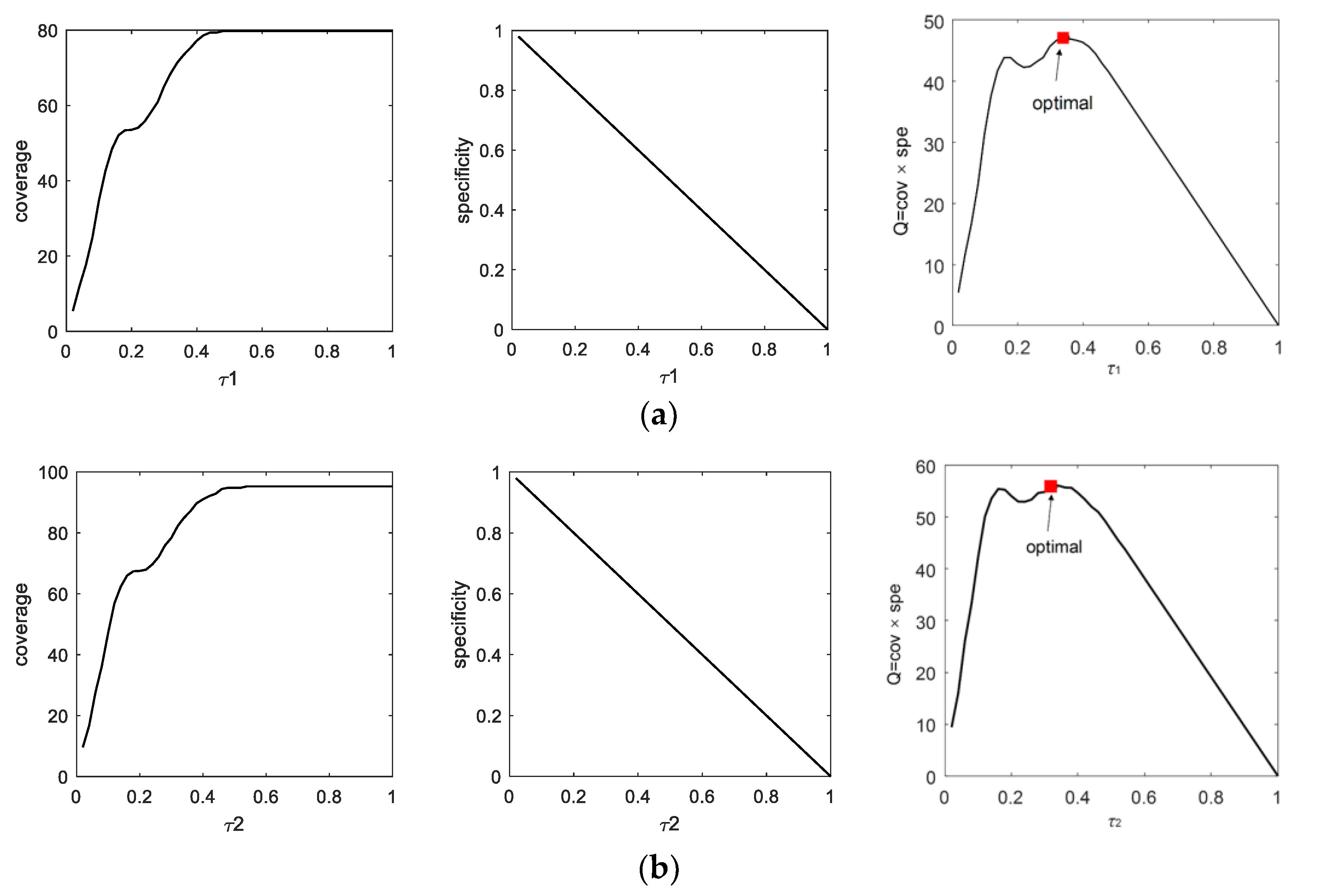
By uniformizing the data into [0, 1], the FCM algorithm is utilized to classify the original data according to Section 2. Then, two fuzzy clusters are generated with prototypes of v_A = 0.2800 and v_B = 0.6699. When mapping them in the original domain, their values are v_A = −2.0736 and v_B = 2.0423 which are consistent with the distribution of the given synthetic data. Moreover, the membership matrix U through FCM is calculated. Figure 3b shows the distribution of memberships to two clusters. Then, according to the criterion in (7), the prototype of the uncertain region between two clusters is determined as the median point x₀ = 0.4737. Next, based on the processes of constructing the uncertain granule in a one-dimensional dataset, two size parameters (τ₁ and τ₂) are calculated using justifiable granulating, as shown in Figure 4.

Figure 4 shows the values of cov(τ), spe(τ) and their product Q = spe(τ) × cov(τ) at different values of the size parameter τ. Here, the parameter β is set to 1, and the final size of the uncertain region is determined as [x₀ − τ₁, x₀ + τ₂] = [0.1337, 0.8137]. It is known that the optimal uncertain region under β = 1 is large, which may generate huge cost in (29). The other challenge in a three-way decision is that it is not clear which points are uncertain and how many data points are true uncertain data. Therefore, to address this problem, we can assume a proportion (E_ur) of data as uncertain data, then set constraints to determine the optimal size parameters for constructing the uncertain region. By forming new classification rules with consideration of the constructed uncertain granule, four metrices in (24)–(27) are calculated for performance analysis, as presented below.

It is found from the results of

Table 2. Performance of three-way decision in one-dimensional synthetic data.

	[x0 − τ1, x0 + τ2]	Acc	R	P	Emis
Eur = 0%	/	0.9830	0.9830	0.9830	0.0170
Eur = 5%	[0.4437, 0.5237]	0.9937	0.9937	0.9937	0.0063
Eur = 10%	[0.4237, 0.5337]	0.9957	0.9957	0.9957	0.0043
Eur = 15%	[0.3737, 0.5637]	0.9988	0.9988	0.9988	0.0012
Eur = 20%	[0.3637, 0.5837]	0.9988	0.9987	0.9988	0.0012
Conventional way		0.9942	0.9942	0.9942	0.0058

that, when the value of E_ur increases, the size of the uncertain region increases, implying more uncertain points are taken for “clerical review”. Values of metrics (Acc, R, P, E_mis) for evaluating classification performance are also improved with the increasing of E_ur. Moreover, as the proportion of uncertain data increases to more than 15%, the improvement of evaluation metrics has no big changes. Therefore, with consideration of computing overhead, there should be a trade-off between performance and cost to select suitable parameters in practical three-way decision processes. For example, in this case, system operators can choose E_ur = 15% as the parameters in a decision based on the results of Table 2.

On the other hand, it is noted from Table 2 that there is no uncertain region considered when E_ur = 0%. Actually, the method degenerates to a traditional two-way decision under this case. Moreover, to compare with the conventional three-way decision, we can choose data within the membership range of [0.45, 0.55] consisting in the uncertain region; the performance is also added to Table 2. It is seen that the conventional method can outperform E_ur = 5% under the given fuzzy set describing uncertainty, which the proposed method can have a flexible operation, and it can outperform the conventional way with better parameters describing uncertain regions.

5.2. Synthetic Two-Dimensional Data

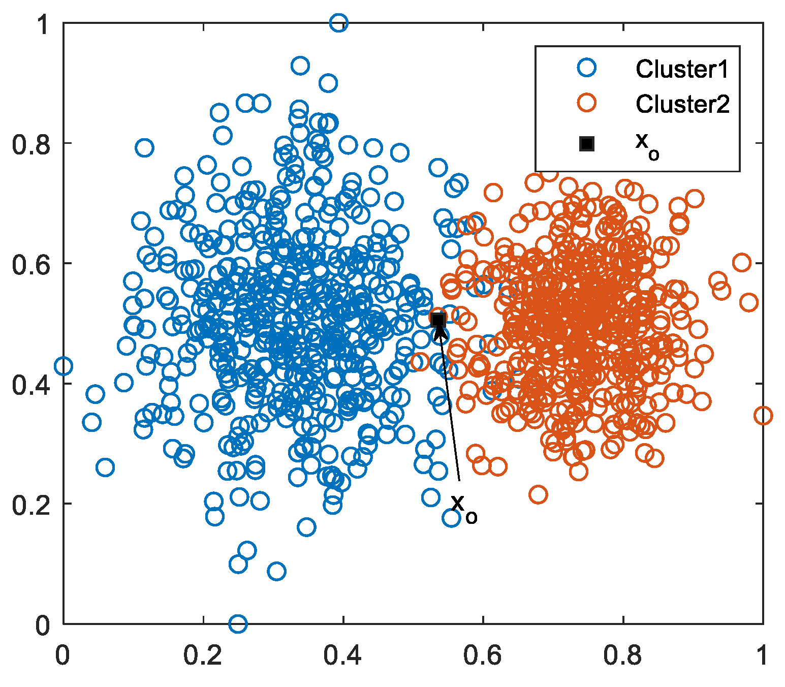
Considering the two-dimensional data space is a representative of high-dimensional data space, a synthetic dataset is generated to study the proposed method on the high-dimensional case. Similar to the one-dimensional case, we can generate two clusters of Gaussian random data in a two-dimensional space. As shown in Figure 5, each cluster has a number of 500 data points. By uniformizing the original data into [0, 1]², the centers of two clusters are determined by FCM as v₁ = (0.3319, 0.5087) and v₂ = (0.7389, 0.5022). Then, according to the formula in (14), the prototype of the uncertain region as x₀ = (0.5354, 0.5055) can be determined.

Centering on the prototype x₀, different shapes of information granules can be constructed via different distance functions. In this paper, we can simply assume the hypersphere as the basic granule architecture, then the optimal size of granule for uncertainty description in a three-way decision is determined via the optimization of coverage and specificity.

As the simplest case, we can set the parameter β as 1 for granule construction, then the variances of coverage and specificity for the uncertainty description are shown in Figure 6. It is seen that coverage (a) and specificity (b) are in conflict to become maximum. Their product (c) can be a useful metric to trade off the optimal size ρ in (18). Therefore, the final size ρ for constructing the uncertain granule is shown in Figure 6. Different from a one-dimensional data space, β = 1 is always the optimal solution in granule construction. When a suitable granule is constructed to describe the uncertain region, the performance and overhead of decision-making will be affected. For example, if a large uncertain granule is constructed, namely implying a large percentage of data requires “clerical review”, then the cost of manual checking will certainty increase, and even the performance on three-way decision might be improved.

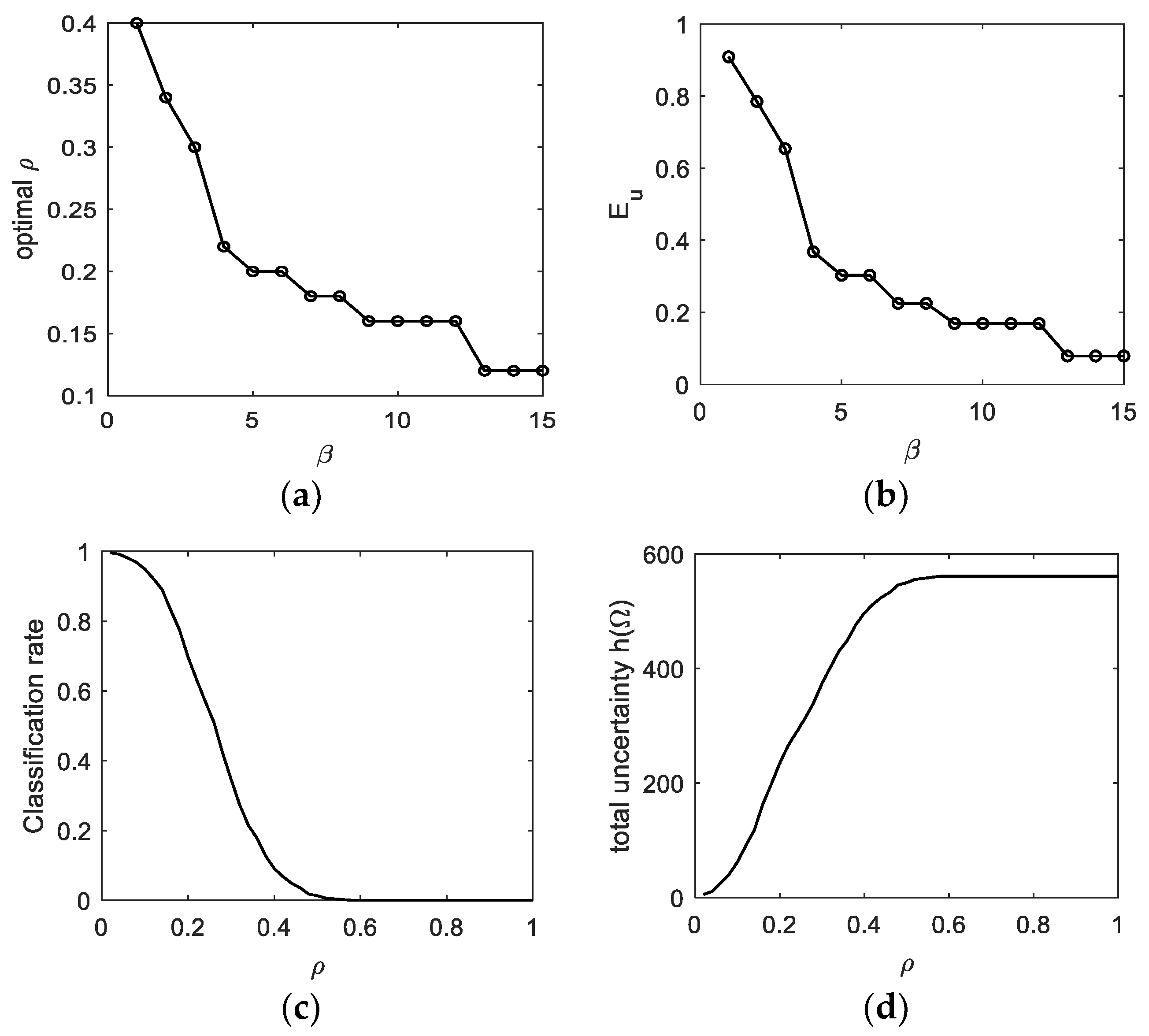
With consideration of this issue, here we implement experiments on using different β to optimize the granule’s size ρ, as shown in Figure 7a,b. Moreover, to discuss the performance of classification with different uncertain regions, values of metrics under different sizes of uncertain granules are shown in Figure 7c,d.

Figure 7a,b shows the values of optimal granule radius ρ and the percentage of points within the uncertain region (i.e., E_ur) at a different parameter β, respectively. It is seen that, when the value of β increases, fewer points within the uncertain region, namely the optimal size of ρ, will decrease. In Figure 7c,d, the classification rate and the total entropy of the uncertain region via (10) are shown at different radius parameter ρ. It is seen that when the value of β increases, the optimal values of ρ and E_ur correspondingly decrease. That is to say, when the uncertain region size increases, the uncertainty contained by the constructed granule increases but the classification rate decreases. For the well-performed classification rules, both the classification rate and the uncertainty of points for “clerical review” should be decided properly. Therefore, by setting different values of E_ur as a constraint condition, uncertain granules are constructed optimally and utilized in the formation of classification rules. The classification performance is reflected by metrics in (24)–(27), as presented in the following table.

According to the results of

Table 3. Performance of decision-making on two-dimensional data.

	β	Acc	R	P	Emis
Eur = 0%	\	0.9640	0.9639	0.9647	0.0360
Eur = 10%	18.74	0.9808	0.9807	0.9812	0.0192
Eur = 20%	12.97	0.9854	0.9855	0.9856	0.0146
Eur = 30%	10.02	0.9905	0.9905	0.9907	0.0095
Eur = 40%	5.39	0.9921	0.9920	0.9922	0.0079
Eur = 50%	5.39	0.9921	0.9920	0.9922	0.0079
Conventional way		0.9913	0.9915	0.9917	0.0087

, a conclusion the same as that from Table 2 is obtained, i.e., when fewer uncertain points are checked for “clerical review”, the values of metrics (Acc, R, P) will decrease and those of E_mis will increase. Moreover, in Table 2, the traditional two-way decision can be expressed by E_ur = 0%, and the conventional method based on fuzzy set describing uncertainty is also added, which sets the membership range [0.45, 0.55] as the uncertain region. Through the comparison, we can see that the proposed method can outperform the traditional two-way decision with consideration of a certain proportion of uncertain data. The conventional fuzzy-set-based method also performs well since the synthetic data is simple and suitable for fuzzy set analysis, but it may encounter difficulties facing data with complex distribution. The proposed method can still have a better performance if set up with suitable parameters in this case.

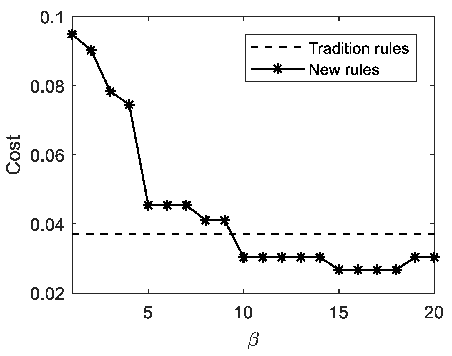
Moreover, it is also seen from Table 3 that a trade-off is required to balance the cost of misclassification and manual recognition. For example, assuming the cost coefficients are set as α = 0.1 and γ = 1, then the cost of classification rules under different sizes of uncertain regions is shown as seen below.

Figure 8 shows the values of cost in (29) with different β, which can also reflect the variance of uncertain granule size in Figure 7. It is seen that when β = 10 with the given coefficients, the classification rules with consideration of uncertain regions will cost less than traditional classification rules. Therefore, combining the results of Table 3 and Figure 8, we can choose E_ur = 30% as the uncertain region size, then both the accuracy and cost can achieve the satisfactory requirement in the practical three-way decision-making process.

5.3. Publicly-Available Real-World Datasets

To further discuss performance of the proposed method in three-way decision-making, four public real-world datasets [35] are also studied, e.g., Iris data (ID), Seeds data (SD), Wine data (WD) and Thyroid Disease dataset (TDD). Detailed information about these four datasets is presented below:

-

Iris data is a typical dataset for clustering and classification. It has 150 samples and four attributes. The dataset is grouped into three classes.

-

Seeds data has a total of 210 samples of three different varieties of wheat, such as Kama, Rosa and Canadian. It has seven attributes for data analysis.

-

Wine data are from the chemical analysis of wines in Italy. There are 13 constituents detected in three different types of wines. In this paper, a number of 178 samples are used for experimental study.

-

The thyroid disease data includes 215 samples with five attributes. These samples are classified into three classes: normal, suffers from hyperthyroidism and hypothyroidism.

According to the information described above, the parameters of four datasets could be simply summarized in

Table 4. Parameters of four real-world datasets.

	# of Samples	# of Attributes	# of Classes
ID	150	4	3
SD	210	7	3
WD	178	13	3
TDD	215	5	3

.

According to the above description, to form classification rules in three-way decisions, the key factor is to construct granules for uncertainty descriptions. Based on the steps described in Section 3, uncertainty regions should be described aiming at each pair of two classes when orienting to multiple classes-based decision processes. While, considering data distributions of real-world datasets are arbitrary, suitable feature learning should be implemented first. For example, neural-network-based models are used first to learn features rid of structure information, then classification rules considering uncertain data descriptions are formed for three-way decision-making. Referring to the proposed method, the descriptors of uncertainty regions are realized by hypersphere granules which are affected by parameters of ρ and β. Then, classification rules are formed based on these uncertain granules and the original two-way decision. Performances of the final three-way decision process are presented as follows.

Table 5. Performance of three-way decision on the Iris dataset.

	β	Acc	R	P	Emis
Eur = 0%	/	0.9461	0.9459	0.9479	0.0539
Eur = 10%	16.00	0.9634	0.9624	0.9632	0.0366
Eur = 20%	10.74	0.9864	0.9864	0.9864	0.0136
Eur = 30%	4.81	0.9864	0.9864	0.9864	0.0136
Eur = 40%	4.76	0.9902	0.9907	0.9902	0.0098
Eur = 50%	4.60	0.9902	0.9907	0.9902	0.0098

,

Table 6. Performance of three-way decision on the Seeds dataset.

	β	Acc	R	P	Emis
Eur = 0%	/	0.9544	0.9543	0.9558	0.0456
Eur = 10%	25.33	0.9621	0.9622	0.9627	0.0379
Eur = 20%	10.57	0.9692	0.9691	0.9693	0.0308
Eur = 30%	8.51	0.9673	0.9662	0.9684	0.0327
Eur = 40%	7.79	0.9623	0.9602	0.9639	0.0377
Eur = 50%	5.89	0.9805	0.9788	0.9829	0.0195

,

Table 7. Performance of three-way decision on the Wine dataset.

	β	Acc	R	P	Emis
Eur = 0%	/	0.9701	0.9738	0.9685	0.0299
Eur = 10%	14.44	0.9833	0.9846	0.9829	0.0167
Eur = 20%	14.44	0.9833	0.9846	0.9829	0.0167
Eur = 30%	12.50	0.9906	0.9918	0.9893	0.0094
Eur = 40%	8.53	0.9944	0.9952	0.9933	0.0056
Eur = 50%	8.53	0.9944	0.9952	0.9933	0.0056

and

Table 8. Performance of three-way decision on the Thyroid Disease dataset.

	β	Acc	R	P	Emis
Eur = 0%	/	0.9598	0.8871	0.9775	0.0402
Eur = 10%	26.02	0.9710	0.9108	0.9839	0.0290
Eur = 20%	22.44	0.9758	0.9253	0.9867	0.0242
Eur = 30%	16.77	0.9912	0.9630	0.9952	0.0088
Eur = 40%	16.43	0.9896	0.9667	0.9940	0.0104
Eur = 50%	8.91	0.9836	0.9615	0.9902	0.0164

present the performance of three-way decisions on the given four real-world datasets. By setting different proportions of uncertain data in three-way decisions, the parameter β for controlling granule size is optimized and shown in these tables. Then, the metrics of Acc, R, P and E_mis are given out. Here, considering fuzzy sets for describing the uncertain regions among multiple classes are not sure, they are not considered for comparison, but E_ur = 0% is still used to represent the traditional two-way decision. Then, based on the results in the above tables, it is also seen when more uncertain data is considered in three-way decisions, the value of β increases to guarantee suitable granules for uncertain data description. Moreover, the performance of three-way decision-making improves as more data is regarded as uncertain data, namely more data for “clerical review”. In this way, the drawback is the manual cost that will increase under the condition of performance improvement. Therefore, a practical way is to trade off the manual cost and performance. Fortunately, based on results in Table 5, Table 6, Table 7 and Table 8 it is found that the performance improvement becomes delayed when the proportion of uncertain data reaches a threshold. In this way, we can combine the results of the performance and the cost calculation in (28) to select the suitable parameters, and finally to realize a practical three-way decision-making.

6. Conclusions

In this paper, an advanced method for constructing granular classification rules is proposed for three-way decision-making. To implement this method, GrC is applied first to construct information granules for uncertain data. Moreover, information entropy is considered in the GrC process for a better description of uncertainty. Aiming at different types of data, this paper presents the processes of constructing uncertain data descriptors on one-dimensional, high-dimensional and multiple-classes of data step by step. Then, orienting to the general two-way classification problems, the three-way decision rules with consideration of the constructed uncertainty granules are formed and utilized in the decision-making of systems analysis. Experiments on synthetic data (including both one-dimensional and two-dimensional data) and publicly available real-world data are implemented according to the proposed method. Some conclusions can be obtained. First, suitable parameters are required to guarantee the optimal construction of granules for uncertainty descriptions. Second, when more uncertain data are extracted for “clerical review”, the performance of decision-making in classification is improved along with the increase of manual cost. Finally, with the trade-off between cost and accuracy, suitable uncertain data proportions can be determined in practical applications based on numerical results. Overall, the feasibility of the proposed method on uncertainty data description is validated. Moreover, with the help of uncertainty granular descriptors, better classification rules can be formed for guiding three-way decisions in practical industrial system analyses.

In addition to the above contributions, there are still some shortages worth future study. For example, one possible development is to replace information entropy with some better uncertainty metrics. Second, as it says above that trade-off is required between manual cost for checking uncertain data and accuracy, is there any way to optimize them together? This was not discussed in this paper. Moreover, more studies on using FCM in supervised classification and semi-supervised classification require in-depth investigation.

References

1. Antoniadi, A.M.; Du, Y.; Guendouz, Y.; Wei, L.; Mazo, C.; Becker, B.A.; Mooney, C. Current challenges and future opportunities for XAI in machine learning-based clinical decision support systems: A systematic review. Appl. Sci. 2021, 11, 5088. [Google Scholar] [CrossRef]
2. Zhong, J.X.; Li, N.; Kong, W.; Liu, S.; Li, T.H.; Li, G. Graph convolutional label noise cleaner: Train a plug-and-play action classifier for anomaly detection. In Proceedings of the IEEE/CVF Conference on Computer Vision and Pattern Recognition, Long Beach, CA, USA, 16–20 June 2019; pp. 1237–1246. [Google Scholar]
3. Jussupow, E.; Spohrer, K.; Heinzl, A.; Gawlitza, J. Augmenting medical diagnosis decisions? An investigation into physicians’ decision-making process with artificial intelligence. Inf. Syst. Res. 2021, 32, 713–735. [Google Scholar] [CrossRef]
4. Ouyang, T.; Marco, V.S.; Isobe, Y.; Asoh, H.; Oiwa, Y.; Seo, Y. Improved Surprise Adequacy Tools for Corner Case Data Description and Detection. Appl. Sci. 2021, 11, 6826. [Google Scholar] [CrossRef]
5. Jeong, Y. Stochastic Model-Predictive Control with Uncertainty Estimation for Autonomous Driving at Uncontrolled Intersections. Appl. Sci. 2021, 11, 9397. [Google Scholar] [CrossRef]
6. Yang, J.; Yao, Y. A three-way decision based construction of shadowed sets from Atanassov intuitionistic fuzzy sets. Inf. Sci. 2021, 577, 1–21. [Google Scholar] [CrossRef]
7. Baratgin, J.; Politzer, G.; Over, D.E.; Takahashi, T. The psychology of uncertainty and three-valued truth tables. Front. Psychol. 2018, 9, 1479. [Google Scholar] [CrossRef]
8. Maldonado, S.; Peters, G.; Weber, R. Credit scoring using three-way decisions with probabilistic rough sets. Inf. Sci. 2020, 507, 700–714. [Google Scholar] [CrossRef]
9. Sun, B.; Chen, X.; Zhang, L.; Ma, W. Three-way decision making approach to conflict analysis and resolution using probabilistic rough set over two universes. Inf. Sci. 2020, 507, 809–822. [Google Scholar] [CrossRef]
10. Yao, J.; Azam, N. Web-based medical decision support systems for three-way medical decision making with game-theoretic rough sets. IEEE Trans. Fuzzy Syst. 2015, 23, 3–15. [Google Scholar] [CrossRef]
11. Pedrycz, W. Shadowed sets: Representing and processing fuzzy sets. IEEE Trans. Syst. Man Cybern. Part B Cybern. 1998, 28, 103–109. [Google Scholar] [CrossRef]
12. Herbert, J.P.; Yao, J.T. Game-theoretic rough sets. Fundam. Inf. 2011, 108, 267–286. [Google Scholar] [CrossRef]
13. Azam, N.; Yao, J.T. Analyzing uncertainties of probabilistic rough set regions with game-theoretic rough sets. Int. J. Approx. Reason. 2014, 55, 142–155. [Google Scholar] [CrossRef]
14. Ouyang, T.; Shen, X. Online Structural Clustering Based on DBSCAN Extension with Granular Descriptors. Inf. Sci. 2022, 607, 688–704. [Google Scholar] [CrossRef]
15. Yao, J.T.; Vasilakos, A.V.; Pedrycz, W. Granular computing: Perspectives and challenges. IEEE Trans. Cybern. 2013, 43, 1977–1989. [Google Scholar] [CrossRef]
16. Ouyang, T.; Pedrycz, W.; Pizzi, N.J. Record linkage based on a three-way decision with the use of granular descriptors. Expert Syst. Appl. 2019, 122, 16–26. [Google Scholar] [CrossRef]
17. Yao, Y.Y. The superiority of three-way decisions in probabilistic rough set models. Inf. Sci. 2011, 181, 1080–1096. [Google Scholar] [CrossRef]
18. Yao, Y. Three-way decision and granular computing. Int. J. Approx. Reason. 2018, 103, 107–123. [Google Scholar] [CrossRef]
19. Al-Hmouz, R.; Pedrycz, W.; Daqrouq, K.; Morfeq, A. Development of multimodal biometric systems with three-way and fuzzy set-based decision mechanisms. Int. J. Fuzzy Syst. 2018, 20, 128–140. [Google Scholar] [CrossRef]
20. Ouyang, T.; Pedrycz, W.; Pizzi, N.J. Rule-based modeling with DBSCAN-based information granules. IEEE Trans. Cybern. 2019, 51, 3653–3663. [Google Scholar] [CrossRef]
21. Wang, L.D.; Zhao, F.; Guo, H.; Liu, X.; Pedrycz, W. Top-down granulation modeling based on the principle of justifiable granularity. IEEE Trans. Fuzzy Syst. 2020, 30, 701–713. [Google Scholar] [CrossRef]
22. Zhang, X.; Shen, X.; Ouyang, T. Extension of DBSCAN in Online Clustering: An Approach Based on Three-Layer Granular Models. Appl. Sci. 2022, 12, 9402. [Google Scholar] [CrossRef]
23. Zhang, H.; Ma, J.; Jing, J.; Li, P. Fabric defect detection using L0 gradient minimization and fuzzy C-means. Appl. Sci. 2019, 9, 3506. [Google Scholar] [CrossRef] [Green Version]
24. Zhuge, W.; Hou, C.; Peng, S.; Yi, D. Joint consensus and diversity for multi-view semi-supervised classification. Mach. Learn. 2020, 109, 445–465. [Google Scholar] [CrossRef]
25. Toledo-Pérez, D.C.; Rodríguez-Reséndiz, J.; Gómez-Loenzo, R.A.; Jauregui-Correa, J.C. Support vector machine-based EMG signal classification techniques: A review. Appl. Sci. 2019, 9, 4402. [Google Scholar] [CrossRef] [Green Version]
26. He, Y.; Kusiak, A.; Ouyang, T.; Teng, W. Data-driven modeling of truck engine exhaust valve failures: A case study. J. Mech. Sci. Technol. 2017, 31, 2747–2757. [Google Scholar] [CrossRef]
27. Askari, S. Fuzzy C-Means clustering algorithm for data with unequal cluster sizes and contaminated with noise and outliers: Review and development. Expert Syst. Appl. 2021, 165, 113856. [Google Scholar] [CrossRef]
28. Ouyang, T.; Pedrycz, W.; Reyes-Galaviz, O.F.; Pizzi, N.J. Granular description of data structures: A two-phase design. IEEE Trans. Cybern. 2019, 51, 1902–1912. [Google Scholar] [CrossRef]
29. Wang, L.; Wang, Y.; Pedrycz, W. Hesitant 2-tuple linguistic Bonferroni operators and their utilization in group decision making. Appl. Soft Comput. 2019, 77, 653–664. [Google Scholar] [CrossRef]
30. Cabrerizo, F.J.; Al-Hmouz, R.; Morfeq, A.; Martínez, M.Á.; Pedrycz, W.; Herrera-Viedma, E. Estimating incomplete information in group decision making: A framework of granular computing. Appl. Soft Comput. 2020, 86, 105930. [Google Scholar] [CrossRef]
31. Wu, W.; Huang, Y.; Kurachi, R.; Zeng, G.; Xie, G.; Li, R.; Li, K. Sliding window optimized information entropy analysis method for intrusion detection on in-vehicle networks. IEEE Access 2018, 6, 45233–45245. [Google Scholar] [CrossRef]
32. Ouyang, T. Structural rule-based modeling with granular computing. Appl. Soft Comput. 2022, 128, 109519. [Google Scholar] [CrossRef]
33. Xu, J.; Zhang, Y.; Miao, D. Three-way confusion matrix for classification: A measure driven view. Inf. Sci. 2020, 507, 772–794. [Google Scholar] [CrossRef]
34. Xiong, Y.; Zha, X.; Qin, L.; Ouyang, T.; Xia, T. Research on wind power ramp events prediction based on strongly convective weather classification. IET Renew. Power Gener. 2017, 11, 1278–1285. [Google Scholar] [CrossRef]
35. UCI Datasets. Available online: https://archive.ics.uci.edu/ml/datasets.php (accessed on 25 May 2022).
Figure 1. Diagram of uncertain data distribution in decision-making. (a) labeled data; (b) unlabeled data; (c) semi-labeled data.
Applsci 12 11381 g001
Figure 2. Diagram of uncertain data in one-dimensional data space.
Applsci 12 11381 g002
Figure 3. Distribution of one-dimensional synthetic data. (a) Original distribution; (b) FCM clustering and membership distribution.
Applsci 12 11381 g003
Figure 4. Variances of coverage, specificity and their product. (a) τ1; (b) τ2.
Applsci 12 11381 g004
Figure 5. Synthetic two-dimensional data.
Applsci 12 11381 g005
Figure 6. Performance of different granule sizes.
Applsci 12 11381 g006
Figure 7. Performance of different parameters in uncertain granule construction. (a) optimal ρ vs β; (b) Eur vs. β; (c) classification rate vs. ρ; (d) uncertainty h(Ω) vs. ρ.
Applsci 12 11381 g007
Figure 8. Comparative results of the cost of different rules.
Applsci 12 11381 g008