Nonlinear Model Predictive Control with Terminal Cost for Autonomous Vehicles Trajectory Follow

Abstract

This paper presents a nonlinear model predictive control with terminal cost (NMPC–WTC) algorithm and its open/closed-loop system analysis and simulation validation for accurate and stable path tracking of autonomous vehicles. The path tracking issue is formulated as an optimal control problem. In order to improve the squeezing phenomenon of traditional NMPC, a discrete-time nonlinear model predictive controller with terminal cost is then designed, in which the state error of last step is augmented. The cost function of NMPC–WTC consists of two parts: (1) the traditional NMPC cost function responding to tracking errors and controller output, and (2) the augmented terminal cost. The algorithm was implemented on CasADi numerical optimization framework, which is free, open-source and developed for nonlinear optimization. The open-loop and closed-loop simulation results are then presented to demonstrate the improved performance in tracking accuracy and stability compared to traditional model predictive controller.

1. Introduction

In recent years, with the development of lidar, millimeter-wave radar, depth camera and AI technology, self-driving technology is also constantly improving. At the same time, a considerable number of domestic and foreign companies and research institutions have invested huge research and development funds and manpower in self-driving technology to conduct research. There is thus reason to believe that self-driving vehicles will gradually enter our lives in the near future with the advancement of self-driving technology and the gradual improvement of laws, regulations and user acceptance. In addition, the superiority of self-driving vehicles over traditional vehicles is also obvious, with one of the most obvious superiorities being that they can reduce traffic accidents and ease traffic congestion [1].

In order to achieve self-driving, self-driving vehicles often have a set of decision-making systems, which are mainly composed of the following function modules: route planning, behavioral decision-making, motion planning, and path tracking [2]. First of all, the vehicle obtains an optimal route from the starting point to the end point according to the current position and road network information. Secondly, the vehicle makes specific behavior decisions such as lane changing, parking, overtaking and so on in accordance with the current environment. Then the vehicle plans a rational path. Finally, the vehicle gives a reasonable control signal according to the current position and the reference path to achieve path tracking.

Unmanned path tracking and vehicle control are the last and indispensable part of self-driving. The crux of them can be summarized as the establishment of vehicle models and the design of control algorithms. Vehicle models include kinematic bicycle models, dynamic bicycle models [3] and so on. And some typical control algorithms include model predictive control [4,5], linear quadratic optimal control [6], PID control [7] and adaptive control [8], etc.

In recent years, nonlinear model predictive control has been widely used in path tracking of self-driving vehicles, nevertheless, most of the current researches use the method of linear expansion at the trajectory reference point, without considering the stability of nonlinear model predictive control. Kühne et al. [4] adopted the kinematics model of self-driving vehicles, and linearly expanded the nonlinear vehicle kinematics model at the trajectory reference point, established a linearized model predictive controller, and finally converted it into a Quadratic Programming (QP) solution. Falcone, P. and Liu, W.F. [9,10,11] pointed out that nonlinear model predictive control (NMPC) is a variant of model predictive control (MPC), which is mainly applicable to the nonlinear control system or the case that is inconvenient to linearize. In common with linearized MPC, NMPC needs to iteratively solve the optimal control problem in a finite time domain. However, due to the nonlinearity of the system, these problems are not necessarily non-convex. Wang, H. et al. [12] proposed a Particle Swarm Optimization (PSO) algorithm to change the MPC predictive control step size in real time to study the influence of the MPC predictive step size on vehicle path tracking. Bai, G. et al. [13] proposed a nonlinear model predictive control algorithm, which verifies the feasibility of nonlinear model predictive control in vehicle path tracking. Chu, D. et al. [14] proposed a model predictive controller with a PID feedback controller to improve the tracking accuracy of the model predictive control in the path tracking process, so that the state error tended to zero during the path tracking process. Qin, S.J. et al. [15] gave a summary of MPC theoretical research, and it is pointed out that the stability of the MPC controller can be enhanced with tail-end contraction constraints, while lead to an accompanying increase in the computing time. Amrit, R. et al. [16] used the method of adding constraints in the terminal area instead of adding contraction constraints at the terminal point to improve the MPC, and gave the open-loop control results and closed-loop control results of model predictive control, which verifies the stability of tail-end constraints. Koehler, J. et al. [17] proposed a nonlinear model predictive control with parametric tail-end contraction constraints; in addition, experiments showed that the control effect of model predictive controller with tail-end contraction constraints is significantly better than that of model predictive controller without tail-end contraction constraints. Köhler, J. et al. [18] provided a stability and performance analysis for nonlinear model predictive control schemes subject to input constraints.

According to previous research, we can find that the theoretical research on NMPC with terminal cost has been perfected, and this method contributes to the stability of the MPC controller [19]. The paper [19] has proved that suitable terminal cost will make the controller more stable. What’s more, traditional NMPC has been widely used in path tracking, but the accuracy of traditional NMPC-based path tracking method is a problem that the industry needs to solve urgently.

Aiming at the existing problems, the main contributions of this study are summarized as follows: (1) A nonlinear model predictive control with terminal cost (NMPC–WTC) path tracking method is proposed, in order to make the vehicle converge to the planned trajectory more quickly and smoothly. The proposed path tracking method can improve the stability of controller, and the error of path tracking is below 0.02 m in our simulation. (2) The effectiveness of the algorithm through numerical simulation is proved. The closed-loop and open-loop simulation can validate that the proposed NMPC–WTC path tracking method is better than traditional NMPC path tracking method. (3) The application scenarios of NMPC with terminal cost are analyzed, and the commonly used terminal cost coefficient in engineering is given.

The remainder of this paper is organized as follows: In Section 2, the control block diagram of the trajectory tracking of the self-driving vehicles is proposed, and the kinematic model of the vehicle is given. In Section 3, the penalty function with terminal cost is built, and the MPC problem is transformed into a nonlinear program (NLP) problem, and finally the effectiveness of the algorithm is verified in different scenarios. The paper ends with conclusions in Section 4.

2. Kinematic Bicycle Model for Autonomous Vehicle

The block diagram of the path tracking control of the autonomous vehicle can be seen in the Figure 1.

Firstly, the motion planner calculates a reasonable trajectory ($Z_{ref}$) according to the current vehicle state information (such as vehicle speed, position, etc.) and the current environment information. In this article, a fixed trajectory is regarded as the target trajectory calculated by the motion planner. The same approach is widely used in the paper [3,12]. Secondly, NMPC gives the vehicle’s control commands (such as front wheel angle, vehicle speed, etc.) based on a series of reference paths in the limited time domain. Finally, the vehicle selects the control command ($u_0$) at the next moment as the input of the vehicle model.

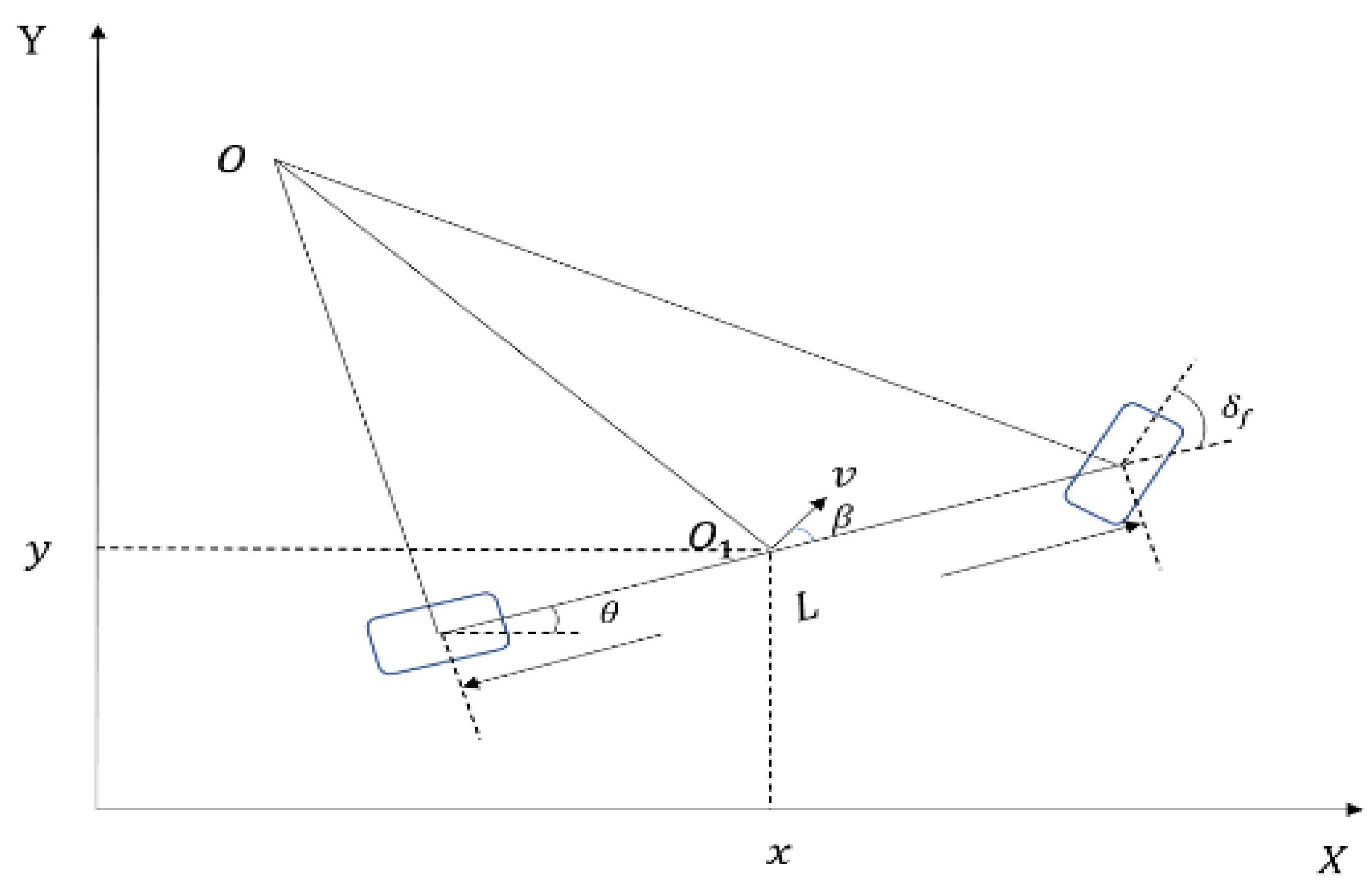
The vehicle kinematics model is shown in Figure 2 below. Here, $L$ represents the wheelbase of the vehicle, $\beta$ represents the side slip angle of the center of mass, $\theta$ represents the heading angle of the vehicle, ${\delta }_f$ represents the front wheel transfer, and the default rear wheel rotation angle is 0; ignoring the lateral sliding of the vehicle, ignoring the slip angle of the vehicle, assuming ${\delta }_f$ is small, the nonlinear continuous time equations that describe a kinematic bicycle model can be expressed as follows [3]:

$$\begin{array}{c}\dot{X}=v\ast \mathit{cos}\left(\theta \right)\end{array}$$

(1)

$$\begin{array}{c}\dot{Y}=v\ast \mathit{sin}\left(\theta \right)\end{array}$$

(2)

$$\begin{array}{c}\omega =\frac{v\ast \mathit{tan}\left({\delta }_f\right)}{L}\end{array}$$

(3)

where $\omega$ is the yaw rate of the vehicle, and L is the wheelbase of the vehicle. The equation above is continuous, which should be discretized.

$Z=\left[X,Y,\theta \right]$ is taken as output of the nonlinear vehicle model, and $u=\left[v,{\delta }_f\right]$ is treated as input of the nonlinear vehicle model, the equation above can thus be expressed as follows:

$$\begin{array}{c}\dot{Z}=f\left(Z,u\right)\end{array}$$

(4)

The Continuous State Space Equation above cannot be used in MPC, so the equation is discretized as follows:

$$\begin{array}{c}Z\left(k+1\right)=A_{k,t}Z\left(k\right)+B_{k,t}\end{array}$$

(5)

In the Equation (5), $A_{k,t}=\left[\begin{array}{ccc}1& 0& 0\\ 0& 1& 0\\ 0& 0& 1\end{array}\right]$;$B_{k,t}=T\left[\begin{array}{c} v cos\theta \\ v sin\theta \\ v tan {\delta }_f/L \end{array}\right]$; T is the sample time, which can be set as 10 ms or 20 ms.

3. Controller Design and Numerical Simulation Verification

3.1. Controller Design

Usually, the NMPC controller converts the path tracking problem into a constrained NLP (Nonlinear Program) problem in the finite time domain. The problem is transformed as follows:

$$\begin{array}{c}\mathit{min}J={\displaystyle \sum _{i=0}^{N_P}}{\left(Z_i-z_{ref,i}\right)}^{T}Q\left(Z_i-z_{ref,i}\right)+u_i^{T}R{u}_i\end{array}$$

(6)

$$s.t. Z_0=Z_t$$

$$Z_{i+1}=f\left(Z_i,u_i\right),i=0,1,2,3\dots \dots .N_p$$

$$u_{min}\le u_i\le u_{max},i=0,1,2,3\dots \dots .N_p$$

$${\dot{u}}_{min}\le \left(u_{i+1}-u_i\right)/T\le {\dot{u}}_{max},i=0,1,2,3\dots \dots .N_p$$

where $J$ is the cost function; $u_{min}, u_{max},{\dot{u}}_{min},{\dot{u}}_{max}$ are the speed, angle, acceleration, and front wheel angle rate constraints; $Z_{i+1}=f\left(Z_i,u_i\right)$ is the differential equation constraint; and the matrix Q and the matrix R are diagonal matrices with weights greater than 0, respectively. In this article, Q = diag(10,10,10), R = diag(1,0.1). In order to achieve a high-precision tracking and planning path of the vehicle and make the controller have high control stability, we propose NMPC with terminal cost, so that the vehicle can better converge to the reference path. Its cost function format is as follows:

$$\begin{array}{c}J=J_{N_p}+{\displaystyle \sum _{i=0}^{N_P-1}}\left[{\left(Z_i-z_{ref,i}\right)}^{T}Q\left(Z_i-z_{ref,i}\right)+u_i^{T}R{u}_i\right]\end{array}$$

(7)

$$\begin{array}{c}{J}_{N_p}=\alpha \ast {\left(Z_{N_p}-z_{ref,N_p}\right)}^{T}Q\left(Z_{N_p}-z_{ref,N_p}\right)+u_{N_p}^{T}R{u}_{N_p}\end{array}$$

(8)

$$s.t. Z_0=Z_t$$

$$Z_{i+1}=f\left(Z_i,u_i\right),i=0,1,2,3\dots \dots .N_p$$

$$u_{min}\le u_i\le u_{max},i=0,1,2,3\dots \dots .N_p$$

$${\dot{u}}_{min}\le \left(u_{i+1}-u_i\right)/T\le {\dot{u}}_{max},i=0,1,2,3\dots \dots .N_p$$

In the Equation (9), $\alpha$ is the terminal cost coefficient greater than 1. The above problems can be solved under the CasADi framework. CasADi can solve QP (quadratic programming) problems and NLP (nonlinear programming) problems, and has Matlab, Python and C++ interfaces, which have been widely used in engineering [20]. The advantage of using CasADi is that only the decision variable, the range of the decision variable and the cost function are needed to set, and then we can quickly solve the optimization problem, which allows us to focus on the design of the cost function formulation. After completing the solution of the above equation in each control cycle, a series of control inputs in the prediction time domain are obtained:

$$\begin{array}{c}{u}^{*}={\left[u_0,u_1,u_2,u_3,\dots ..u_{N_p-1}\right]}^T\end{array}$$

(9)

If the control horizon of the controller is 1, then $u_0$ will be taken as the input of the controller at the next moment, and the input of the controller will be recalculated at the next moment to update $u^{*}$. If the control horizon of the controller is 3, then the input the controller will take will be: [$u_0,u_1,u_2$], the controller will update $u^{*}$ after 3Ts. The control horizon is denoted as $N_c$.

In the vehicle routing control system, $u=\left[v,{\delta }_f\right]$, then the above formula can be written as:

$$\begin{array}{c}{u}^{*}={\left[\left[v_0,{\delta }_{f_0}\right],\left[v_1,{\delta }_{f_1}\right]\dots \dots \left[v_{N_p-1},{\delta }_{f_{N_p-1}}\right]\right]}^T\end{array}$$

(10)

In engineering practice, if the MCU (Microcontroller Unit) has enough computing power, we can choose the larger predictive horizon $N_p$ (such as $N_p$ = 60) and the smaller control horizon $N_c$ according to the study [21]. The larger the value of the predictive horizon, the more stable and accurate the value solved by MPC is. What’ more, the value range of $N_p$ can usually be between 10~20 to balance the calculation time and calculation accuracy, as noted in these studies [22,23]. According to the basic principles of model predictive control, the first element $u_0$ in the control sequence is used as the actual control quantity to act on the system, namely

$$\begin{array}{c}{u}_0={\left[v_0,{\delta }_{f_0}\right]}^T\end{array}$$

(11)

After entering the next control cycle, the above process is repeated, and the trajectory tracking control of the vehicle is realized in this cycle.

3.2. Algorithm Numerical Verification

The numerical simulation of vehicle path tracking is realized based on Matlab, and the specific simulation conditions are shown in

Table 1. Basic parameters of vehicle model.

The Parameter of Vehicle Model	Value
Wheelbase, L	2.9 m
Value range of front wheel angle, ${\delta }_f$	−0.26 rad~0.26 rad
Longitudinal speed of the vehicle, v	0~33.3 m/s
Forward Euler discrete time, T	200 ms
Predictive horizon, $N_p$	20

.

3.2.1. Control Open-Loop Simulation

Our study included model predictive control open-loop simulation, that is, taking the planned trajectory as the input, after solving a series of control inputs of the vehicle in the future limited time domain, and we applied all the control inputs to the vehicle. The same simulation is also covered in the paper [3], and the higher the open-loop path tracking accuracy, the higher the closed-loop path tracking accuracy. Inspired by the paper [3], the open-loop path tracking simulation comparison simulation based on NMPC and the proposed NMPC–WTC path tracking method is carried out in Section 3.2.1, and the closed-loop path tracing simulation comparison is carried out in Section 3.2.2.

The commonly used cubic Bezier curve is chosen as the planned trajectory of the vehicle, and the slope of the planned trajectory is used as the reference heading angle to verify the effectiveness of the proposed algorithm.

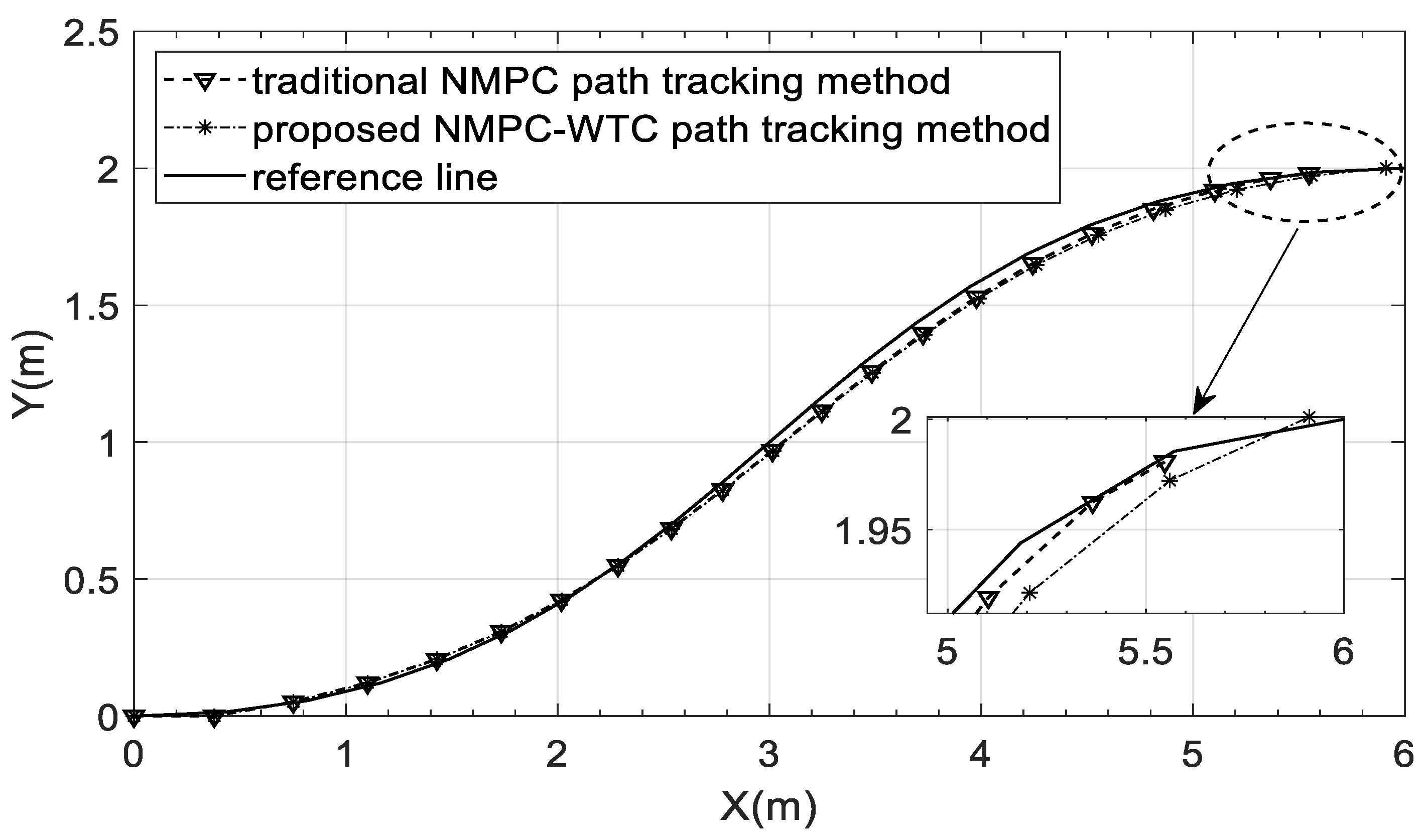
We chose the path tracking diagram of the vehicle as shown in Figure 3. The black solid line in Figure 3 is the reference trajectory. The dotted line with star marker in Figure 3 is the tracking trajectory of proposed NMPC–WTC path tracking method and the dotted line with triangle marker is the tracking trajectory of traditional NMPC path tracking method.

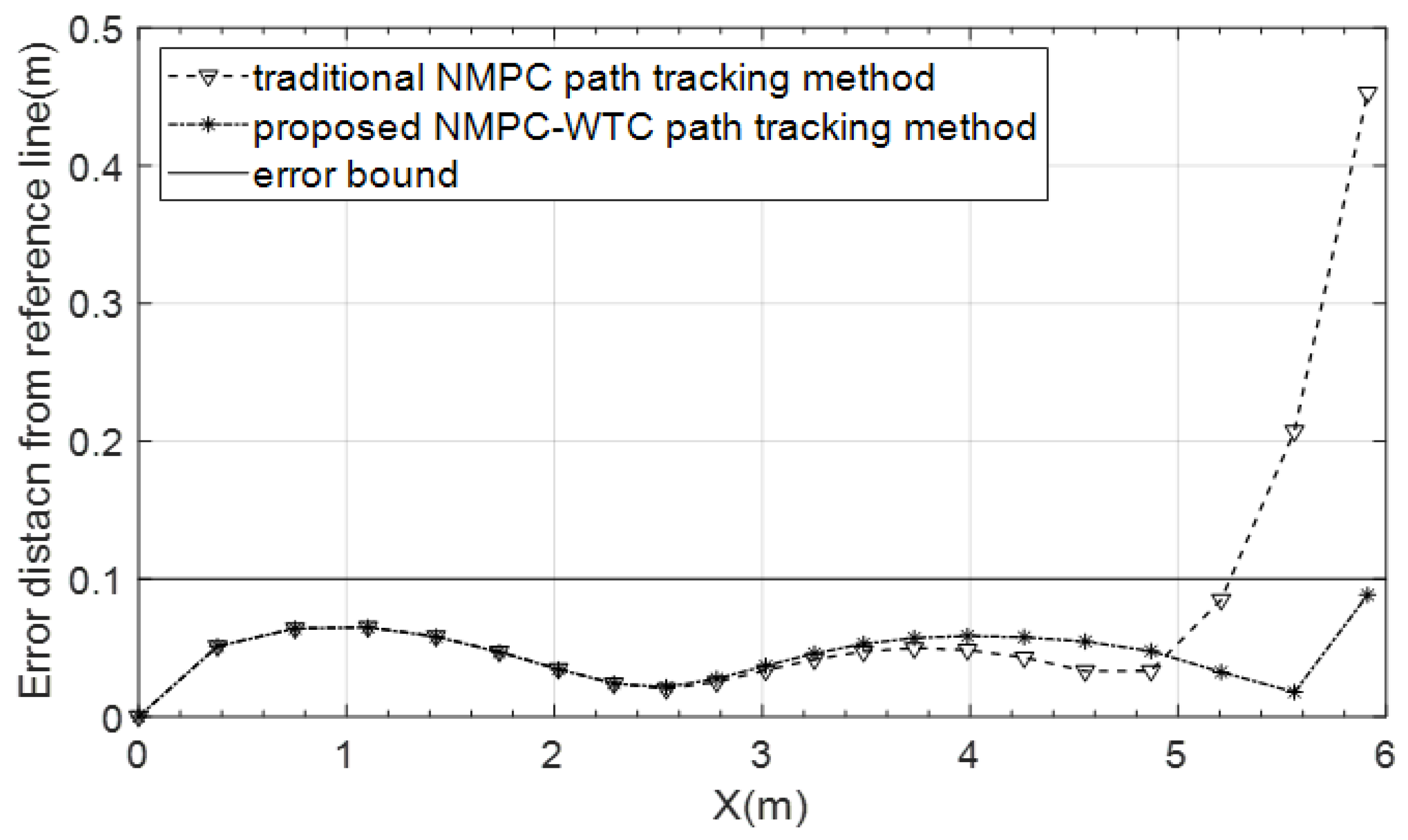
In Figure 3, the NMPC controller without terminal cost will lead to a squeezing phenomenon at the end of the predictive horizon, which will cause the vehicle to deviate from the reference trajectory. The squeezing phenomenon means that the tracking error will increase as the prediction step size increases and the error is accumulated. The accumulation and forward propagation along predictive horizon of the error leads to the larger error at the end. The paper [3] also shows that the mean and standard deviation of step n are bigger than step n−1. The step n is equal to 2~4 in paper [3]. Figure 3 and Figure 4 demonstrate that proposed NMPC–WTC path tracking method improves the squeezing phenomenon of traditional NMPC greatly. The open-loop trajectory calculated by the proposed method will converge to reference trajectory eventually.

The error between the control predicted trajectory and the reference trajectory is shown in Figure 4. In open-loop simulation, maximum error in the NMPC-based scenario was reduced by 80%. In order to distinguish the tracking accuracy of the two different path tracking methods significantly, the error bound is used in Figure 3, and the value of error bound is set to 0.1 m.

In Figure 3, we have verified the validity of the terminal cost, but we have not explained how to set value of the terminal cost coefficient α. In Figure 3, the value of α is 10. We will verify the influence of different terminal cost coefficients on the open-loop prediction trajectory under the same planning trajectory.

3.2.2. The Influence of Terminal Cost Coefficient

The time required to solve the MPC problem is one of the issues of concern when designing MPC. Based on this, the effect of different terminal cost weights on the solution time is verified by different terminal cost coefficients. The experimental results are shown in

Table 2. The solution time of NMPC.

The Value of Terminal Cost Coefficient (α)	Solution Time
1 (without terminal cost)	0.030 s
2	0.032 s
10	0.043 s
100	0.058 s
500	0.061 s

. The experimental results show that with the terminal cost coefficient increasing, the solution time will be longer. Considering the solution time and solution accuracy, the terminal cost coefficient is usually less than 10.

3.2.3. Control Closed-Loop Simulation

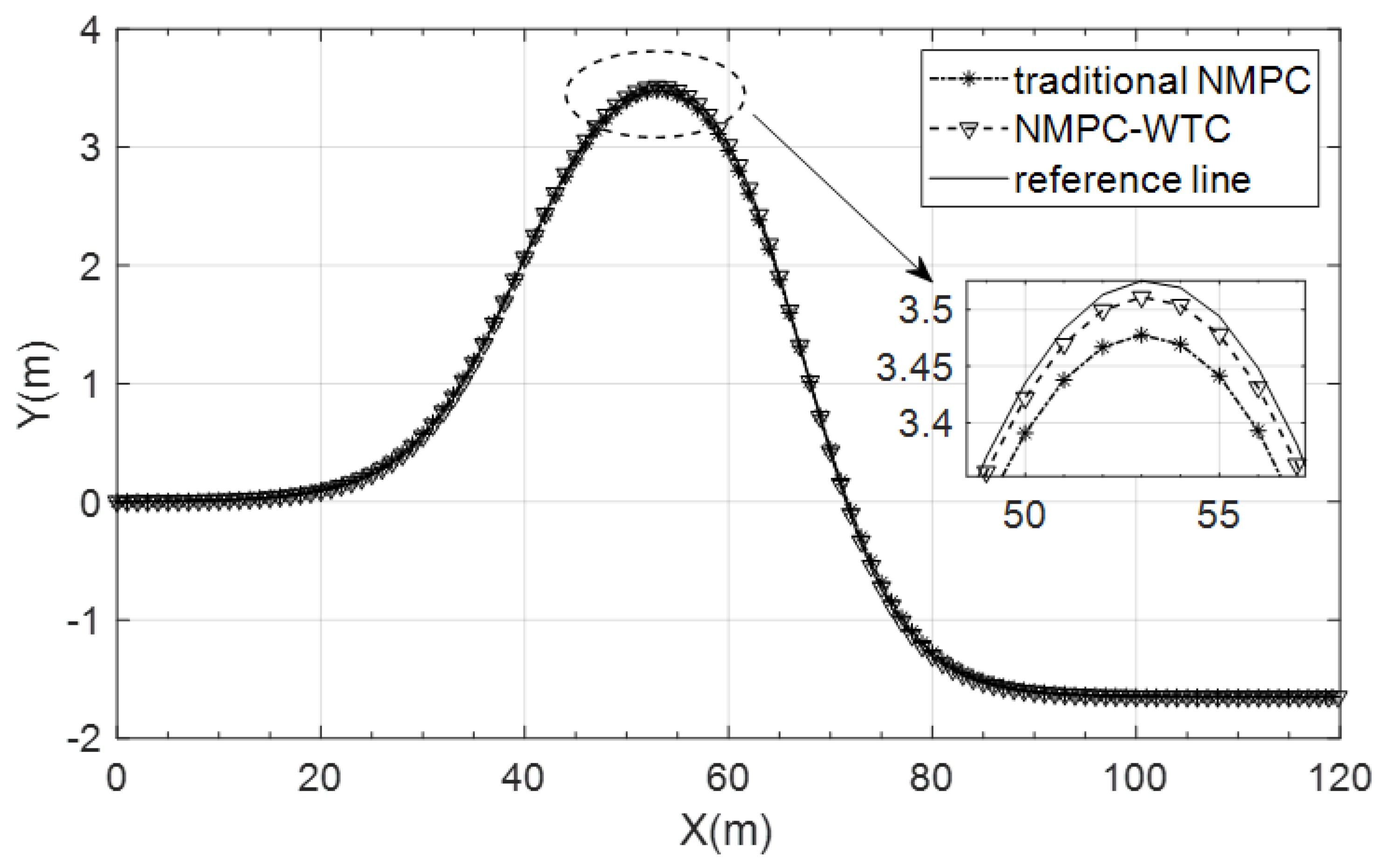
In the stability test of ordinary vehicles, the double-line shift condition is a test section with a high frequency of use. At present, there are also many scholars who use double line shifting as a test of the trajectory tracking ability of unmanned vehicles [11]. We refer to the double line shifting formula in the paper [11] to obtain the reference trajectory and reference heading angle, as shown in Figure 5 below. In this experiment, the control horizon is set as 15, and the predictive horizon is set as 20. Figure 5 verifies the above conclusion in Section 3.2.2. When the control horizon and the prediction horizon are relatively close, the results calculated by NMPC without terminal cost will affect the path tracking accuracy.

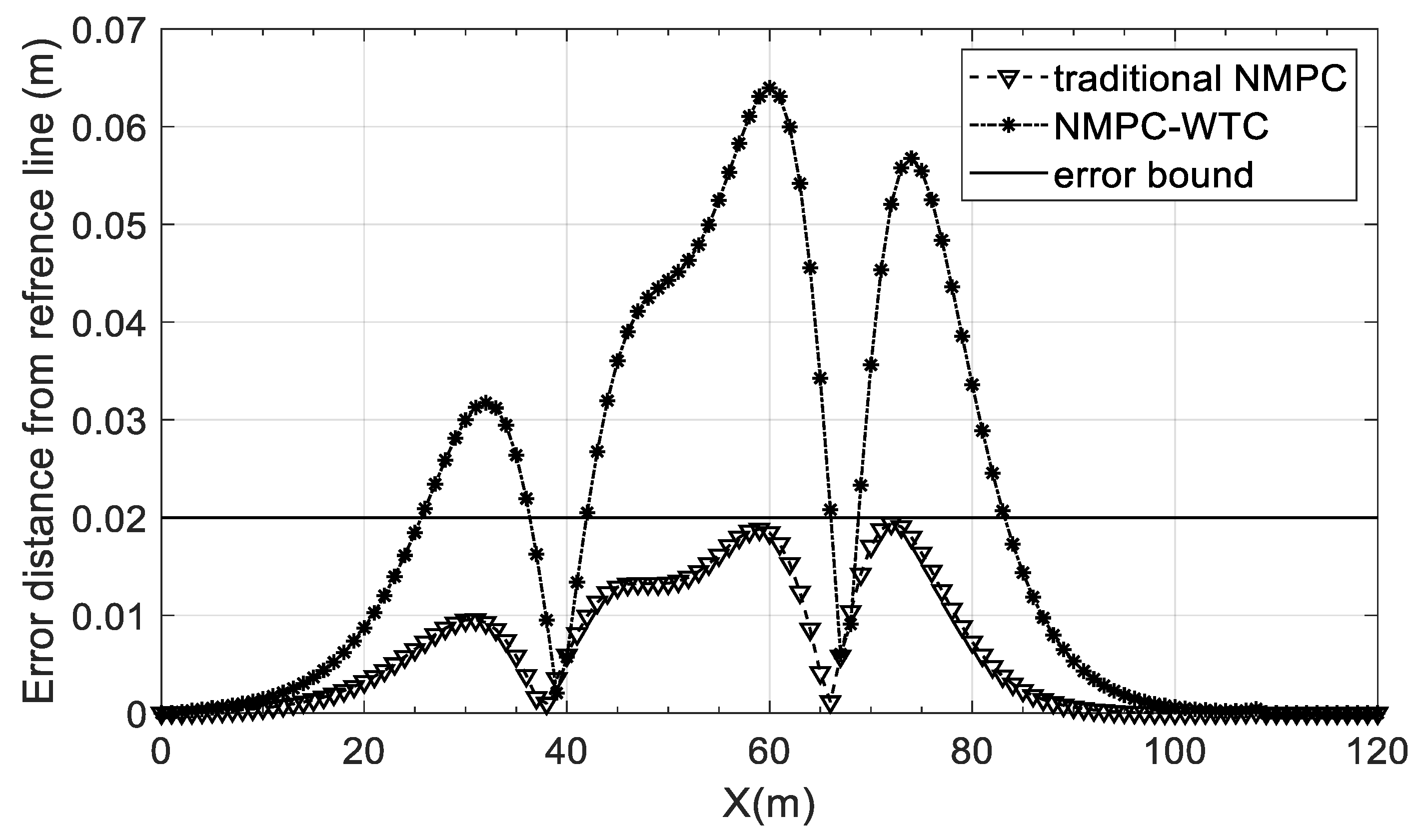
In Figure 6, the NMPC solution with terminal cost is more accurate. In the process of path tracking, the NMPC solver with terminal cost produces a maximum error of 0.02 m, while the path tracking error of the NMPC solver without terminal cost is 0.06 m. Maximum error in the NMPC-based path tracking scenario was reduced by 30% in the simulation. In order to distinguish the tracking accuracy of the two different path tracking methods significantly, the value of error bound in Figure 6 is set to 0.02 m.

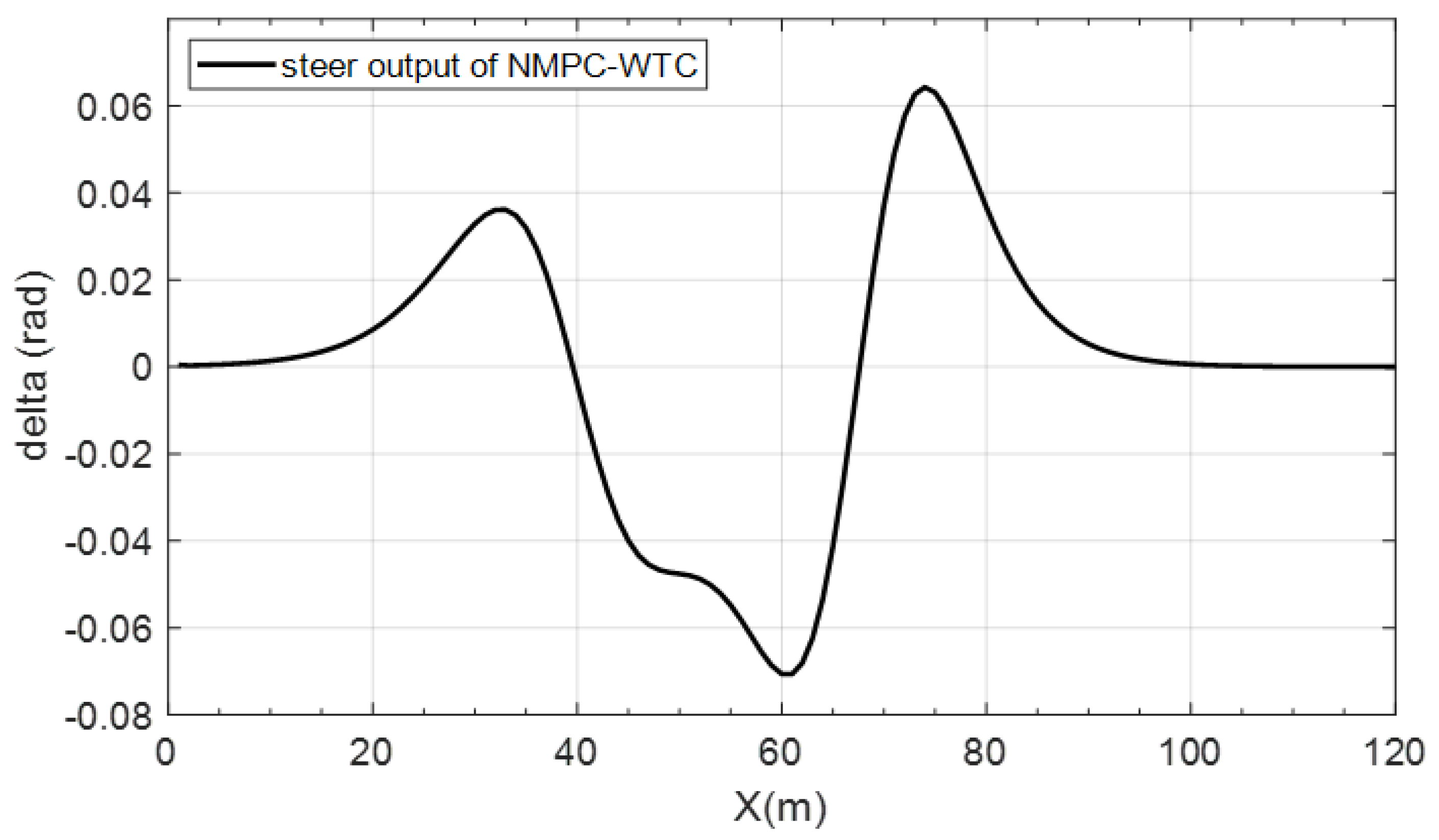
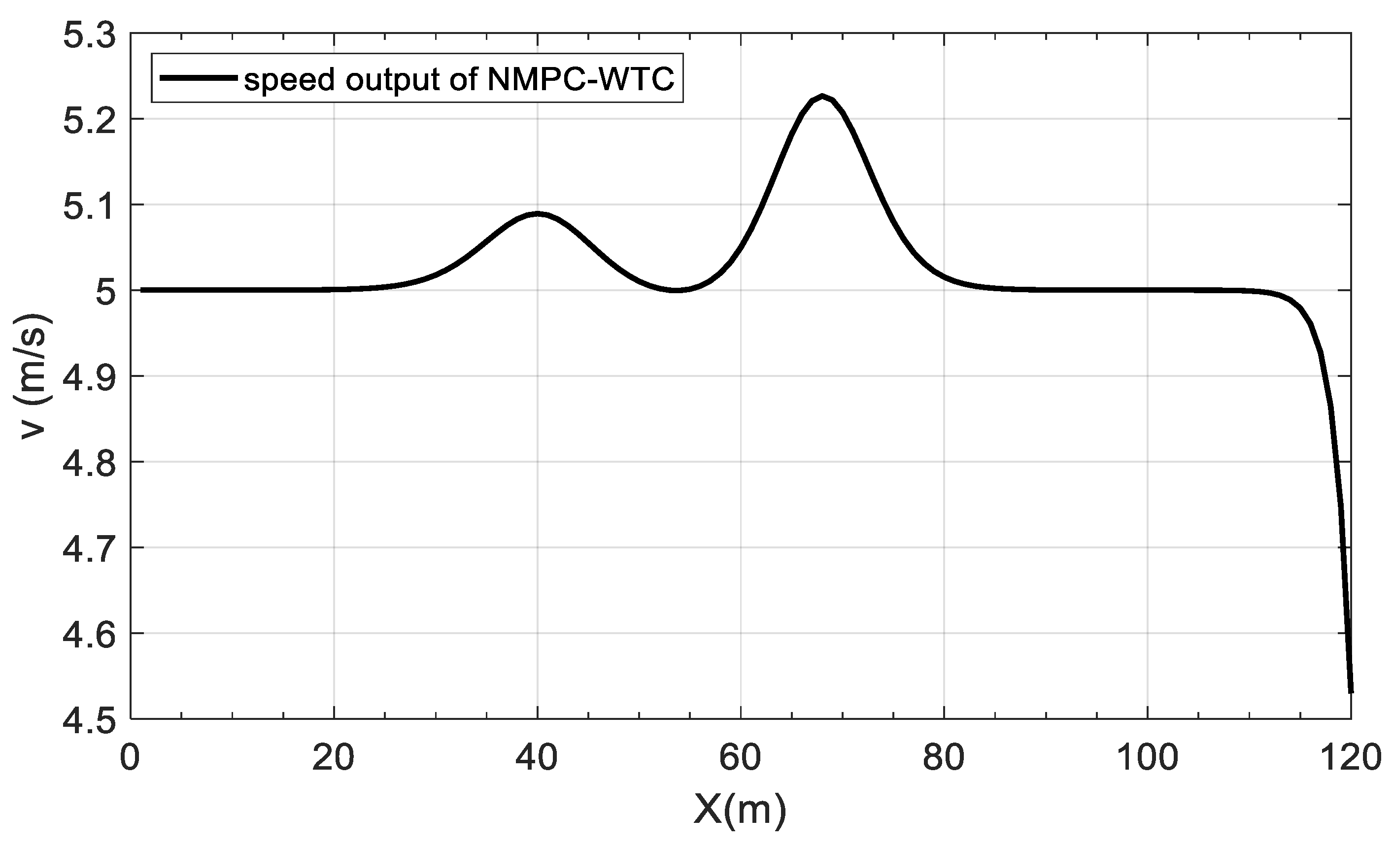
The output of proposed NMPC–WTC path tracking method can be seen in Figure 7 and Figure 8.

4. Conclusions

Comparisons between the nonlinear model predictive control with terminal cost (NMPC–WTC) and traditional NMPC path tracking method were done in order to validate the effectiveness of proposed algorithm. The comparative open-loop simulation fully shows the mechanism of squeezing phenomenon of NMPC and the proposed NMPC–WTC method can improve this phenomenon greatly. The terminal cost will reduce the error at the end greatly. The comparative closed-loop simulation indicates that the traditional NMPC path tracking method will lead to larger error eventually. The results show that the maximum error of the proposed NMPC–WTC path tracking method is reduced by 30% in closed-loop simulation. The computation load simulation shows the limitation of the proposed approach and the commonly used terminal cost coefficient is given.

In future work, the Particle Swarm Optimization algorithm will be used to optimize terminal cost coefficient, which will adjust the terminal cost coefficient automatically and appropriately.

References

1. Alcala, E.; Puig, V.; Quevedo, J.; Cayuela, V.P.; Casin, J.Q. TS-MPC for Autonomous Vehicles Including a TS-MHE-UIO Estimator. IEEE Trans. Veh. Technol. 2019, 68, 6403–6413. [Google Scholar] [CrossRef]
2. Paden, B.; Cap, M.; Yong, S.Z.; Yershov, D.; Frazzoli, E. A Survey of Motion Planning and Control Techniques for Self-Driving Urban Vehicles. IEEE Trans. Intell. Veh. 2016, 1, 33–55. [Google Scholar] [CrossRef] [Green Version]
3. Kong, J.; Pfeiffer, M.; Schildbach, G.; Borrelli, F. Kinematic and dynamic vehicle models for autonomous driving control design. In Proceedings of the 2015 IEEE Intelligent Vehicles Symposium (IV), Seoul, Korea, 28 June–1 July 2015; pp. 1094–1099. [Google Scholar] [CrossRef]
4. Kühne, F.; Lages, W.F.; Silva, J.M. Model Predictive Control of a Mobile Robot Using Linearization. In Proceedings of the Mechatronics and Robotics 2004, Aachen, Germany, 13–15 September 2004. [Google Scholar]
5. Wang, H.; Liu, B.; Ping, X.; An, Q. Path tracking control for autonomous vehicles based on an improved MPC. IEEE Access 2019, 7, 161064–161073. [Google Scholar] [CrossRef]
6. Shuai, Z.; Zhang, H.; Wang, J.; Li, J.; Ouyang, M. Combined AFS and DYC control of four-wheel-independent-drive electric vehicles over CAN network with time-varying delays. IEEE Trans. Veh. Technol. 2013, 63, 591–602. [Google Scholar] [CrossRef]
7. Chen, X.; Bao, Q.; Zhang, B. Research on 4WIS Electric Vehicle Path Tracking Control Based on Adaptive Fuzzy PID Algorithm. In Proceedings of the 2019 Chinese Control Conference (CCC), Guangzhou, China, 27–30 July 2019; pp. 6753–6760. [Google Scholar] [CrossRef]
8. Liu, W.; Wang, R.; Xie, C.; Ye, Q. Investigation on adaptive preview distance path tracking control with directional error compensation. Proc. Inst. Mech. Eng. Part I J. Syst. Control Eng. 2020, 234, 484–500. [Google Scholar] [CrossRef]
9. Findeisen, R.; Allgöwer, F. An introduction to nonlinear model predictive control. In Proceedings of the 21st Benelux Meeting on Systems and Control, Veldhoven, The Netherlands, 19–21 March 2002; Volume 11, pp. 119–141. [Google Scholar]
10. Rafaila, R.C.; Livint, G. Nonlinear model predictive control of autonomous vehicle steering. In Proceedings of the 2015 19th International Conference on System Theory, Control and Computing (ICSTCC), Cheile Gradistei, Romania, 14–16 October 2015; pp. 466–471. [Google Scholar] [CrossRef]
11. Falcone, P.; Eric Tseng, H.; Borrelli, F.; Asgari, J.; Hrovat, D. MPC-based yaw and lateral stabilization via active front steering and braking. Veh. Syst. Dyn. 2008, 46, 611–628. [Google Scholar] [CrossRef]
12. Wang, H.; Wang, Q.; Chen, W.; Zhao, L.; Tan, D. Path tracking based on model predictive control with variable predictive horizon. Trans. Inst. Meas. Control 2021, 43, 014233122110038. [Google Scholar] [CrossRef]
13. Bai, G.; Liu, L.; Meng, Y.; Luo, W.; Gu, Q.; Ma, B. Path Tracking of Mining Vehicles Based on Nonlinear Model Predictive Control. Appl. Sci. 2019, 9, 1372. [Google Scholar] [CrossRef] [Green Version]
14. Chu, D.; Li, H.; Zhao, C.; Zhou, T. Trajectory Tracking of Autonomous Vehicle Based on Model Predictive Control with PID Feedback. IEEE Trans. Intell. Transp. Syst. 2022, 1–12. [Google Scholar] [CrossRef]
15. Qin, S.J.; Badgwell, T.A. Constrained model predictive control: Stability and optimality. Control Eng. Pract. 2003, 11, 733–764. [Google Scholar] [CrossRef]
16. Amrit, R.; Rawlings, J.B.; Angeli, D. Economic optimization using model predictive control with a terminal cost. Ann. Rev. Control 2011, 35, 178–186. [Google Scholar] [CrossRef]
17. Koehler, J.; Muller, M.A.; Allgower, F. A nonlinear model predictive control framework using reference generic terminal ingredients. IEEE Trans. Autom. Control 2019, 65, 3576–3583. [Google Scholar] [CrossRef] [Green Version]
18. Köhler, J.; Zeilinger, M.; Grüne, L. Stability and performance analysis of NMPC: Detectable stage costs and general terminal costs. arXiv 2021, arXiv:2110.11021. [Google Scholar]
19. Borrelli, F.; Bemporad, A.; Morari, M. Predictive Control for Linear and Hybrid Systems; Cambridge University Press: Cambridge, UK, 2017. [Google Scholar]
20. Andersson, J.A.; Gillis, J.; Horn, G.; Rawlings, J.B.; Diehl, M. CasADi: A software framework for nonlinear optimization and optimal control. Math. Program. Comput. 2019, 11, 1–36. [Google Scholar] [CrossRef]
21. Marruedo, D.L.; Alamo, T.; Camacho, E.F. Enlarging the domain of attraction of MPC controller using invariant sets. IFAC Proc. Vol. 2002, 35, 47–52. [Google Scholar] [CrossRef] [Green Version]
22. Sawma, J.; Khatounian, F.; Monmasson, E.; Ghosn, R.; Idkhajine, L. The effect of prediction horizons in MPC for first order linear systems. In Proceedings of the 2018 IEEE International Conference on Industrial Technology (ICIT), Lyon, France, 20–22 February 2018; pp. 316–321. [Google Scholar] [CrossRef]
23. Ma, A.; Liu, K.; Zhang, Q.; Liu, T.; Xia, Y. Event-Triggered Distributed MPC With Variable Prediction Horizon. IEEE Trans. Autom. Control 2021, 66, 4873–4880. [Google Scholar] [CrossRef]
Figure 1. Simplified architecture of vehicle trajectory following.
Applsci 12 11359 g001
Figure 2. Kinematic bicycle model for autonomous vehicle.
Applsci 12 11359 g002
Figure 3. Schematic diagram of vehicle lane changing path tracking.
Applsci 12 11359 g003
Figure 4. Schematic diagram of open-loop prediction error of vehicle lane change.
Applsci 12 11359 g004
Figure 5. Path tracking in double line shifting scenario.
Applsci 12 11359 g005
Figure 6. Path tracking error in double line shifting scenario.
Applsci 12 11359 g006
Figure 7. Steer output of proposed NMPC–WTC path tracking method.
Applsci 12 11359 g007
Figure 8. Speed output of proposed NMPC–WTC path tracking method.
Applsci 12 11359 g008