Abstract
The Industrial Internet of Things (IIoT) has revolutionized businesses by changing the way data are used to make products and services more efficient, reliable, and profitable. To achieve the improvement goals, the IIoT must guarantee the real-time performance of industrial applications such as motion control, by providing stringent quality of service (QoS) assurances for their (industrial applications) communication networks. An application or service may malfunction without adequate network QoS, resulting in potential product failures. Since an acceptable end-to-end delay and low jitter or packet delay variation (PDV) are closely related to quality of service (QoS), their impact is significant in ensuring the real-time performance of industrial applications. Although a communication network topology ensures certain jitter levels, its real-life performance is affected by dynamic traffic due to the changing number of devices, services, and applications present in the communication network. Hence, it is essential to study the jitter experienced by real-time traffic in the presence of background traffic and how it can be maintained within the limits to ensure a certain level of QoS. This paper presents a probabilistic network calculus approach that uses moment-generating functions to analyze the delay and PDV incurred by the traffic flows of interest in a wired packet switched multi-stage network. The presented work derives closed-form, end-to-end, probabilistic performance bounds for delay and PDV for several servers in series in the presence of background traffic. The PDV analysis conducted with the help of a Markovian traffic model for background traffic showed that the parameters from the background traffic significantly impact PDV and that PDV can be maintained under the limits by controlling the shape of the background traffic. For the studied configurations, the model parameters can change the PDV bound from 1 ms to 100 ms. The results indicated the possibility of using the model parameters as a shaper of the background traffic. Thus, the analysis can be beneficial in providing QoS assurances for real-time applications.
1. Introduction
The Industrial Internet of Things (IIoT) promises to achieve improved productivity, reliability, and revenues in the automation business by connecting embedded devices to “the Internet ” [1]. As a global communication infrastructure, the Internet is anticipated to support real-time applications requiring a high level of quality of service (QoS). Industrial systems typically provide real-time and non-real-time services. Real-time services usually have strict QoS constraints not only on delay, but also, even stricter, on jitter or packet delay variation (PDV). PDV is the difference in the end-to-end one-way delay between selected packets in a flow with any lost packets being ignored. The IIoT must guarantee the real-time performance of industrial processes as a product may malfunction or fail in the absence of such assurances. The real-time performance of the IIoT is affected by many subsystems, such as sensor data capture, data processing, communication, production control, and operational activities. In motion control applications, a process is controlled by the message output that is generated from the process loop. Having a constant loop time is a crucial requirement for controlling the process in an efficient manner. Since jitter expresses the amount of deviation from the expected loop response time, in such applications, it is more critical than network speed. Most industrial Ethernet networks claim to have a low jitter. Its real-world performance, however, may differ depending on how much jitter exists in other network devices and how many cascaded devices the packets pass through.
Another category of real-time applications utilizing the Internet in a commercial domain is multi-media applications, e.g., voice over IP (VoIP), streaming video, and online gaming. It is common for real-time voice or video applications to generate continuous traffic streams. For such traffic, jitter is an influential performance metric, which determines how much distortion occurs between a source and a destination through a packet stream in between them [2]. The distortion is as a result of multiple multiplexing operations between network routers and background traffic. It is possible to reduce real-time multi-media service disruptions such as clipped words, disruptions in service, and call drop-outs by maintaining a network jitter below an acceptable level.
Thus, the current and future industrial communication networks involve a high data rate, best-effort traffic, working alongside real-time traffic for time-critical applications with hard deadlines. All time-critical applications require certain levels of QoS for smooth operation. QoS is expressed in terms of one-way delay, jitter, and packet loss. In many such applications, jitter has stricter restrictions to ensure QoS guarantees. Keeping jitter within certain limits is challenging in an ever-expanding communication network due to the growing number of devices, services, and applications. Hence, it is significant to explore the impact of non-real-time services on real-time services from a jitter perspective.
In this paper, we study the end-to-end delay and PDV in a multi-hop wired packet switched network using a network-calculus-based approach and investigate the impact of the network parameters on PDV. The hypothesis of this work is that the PDV experienced by the traffic of interest can be amended by changing the shape of the background traffic. We carried out the analysis to test the validity of this hypothesis. The outcome of the analysis is beneficial in developing approaches for keeping network PDV below certain limits by controlling the network parameters. Traditionally, network calculus facilitates a worst-case analysis of networking queues and allows the derivation of deterministic performance bounds on delays. However, the worst-case scenarios rarely happen in practice. Thus, the deterministic performance bounds are pessimistic and often overestimate the network resources. To overcome this shortcoming, the stochastic or probabilistic branch of network calculus employs statistical multiplexing of independent traffic flows to smooth out burstiness with a high probability. The stochastic network calculus allows the derivation of performance bounds with a certain violation probability. Having derived the performance bounds for a single-hop network, the earlier approaches of deriving end-to-end performance bounds for a multi-hop network involved using an iterative application to add up per-stage delay bounds and concatenating probabilistic service curves. Most of these approaches resulted in loose bounds, and the bounds decreased with the number of stages involved. Easy scaling of stages and the derivation of tighter end-to-end performance bounds for concatenated systems are critical aspects of multi-hop networks. We provide a system theoretic formulation of the probabilistic network calculus with moment-generating functions (MGFs) for general -traffic models, allowing us to estimate multi-hop performance without assuming anything beyond MGFs’ existence and their statistical independence.
The contributions of this work are as follows:
- (1)
- We derived closed-form, end-to-end, probabilistic performance bounds for PDV using MGFs and (min, +) algebra. The limited literature search showed that applying MGFs to derive bounds for PDV is a novel approach. The analytical expression for PDV can be easily scaled to analyze the performance of multi-hop networks.
- (2)
- The delay and PDV analytical expressions were derived using a general traffic model to describe through (of interest) and cross (background) traffic. A wide variety of traffic models can replace the general traffic model. Thus, PDV computation can easily be extended for arrival processes such as periodic, fluid, on–off, and regulated sources.
- (3)
- The analysis based on simulations showed how different network parameters impact end-to-end PDV. The analysis also revealed that, if certain parameters are controlled in a systematic manner, the background traffic can be shaped in a way that results in bounded PDV for the desired traffic. This knowledge can be utilized to shape the background traffic so that PDV can be kept in the desired range by controlling the network parameters.
The paper is organized as follows. First, the related work is presented in Section 2. Section 3 describes the preliminaries of network calculus. Section 4 establishes end-to-end probabilistic bounds for delay and PDV, and Section 5 evaluates the performance based on simulations. Conclusions are provided at the end.
2. Related Work
With their variable and unpredictable performance, networked communication systems suffer from significant bottlenecks in real-time systems: delay and jitter between nodes. The following research on the analytical study of jitter in an IP network has been reported.
A simple analytic approximation was derived for the end-to-end delay, jitter incurred by periodic traffic with a constant packet size by O. Brun et al. [3]. The formula is based on computing the expectation (average value) of a waiting time. The main limit of approximation lies in the assumption of independence with respect to the waiting times of two consecutive packets. This assumption holds only in light of moderate traffic conditions, and hence, the validity range of this formula is limited.
The estimation of jitter experienced by a periodic traffic [4], Poisson arrival [5], and non-Poisson arrival first-come-first-serve (FCFS) queue with a single flow [6] has been proposed in the literature. Further, G. Geleji. et al. [7] reported a jitter analysis of a tagged stream in the presence of a background stream. They defined jitter as the percentile of the inter-arrival time of successive packets at the destination. However, the solution for jitter was obtained numerically, which introduced an error in the computation. Most of these approaches for jitter estimation are based on steady-state analysis methods (SAMs). However, the significant characteristics of jitter, such as the probability distribution, cannot be obtained by a steady-state analysis.
In contrast to SAM-based approaches, S. Thombre et al. [8] presented an analytical expression for the end-to-end delay jitter using a transient queuing analysis. Network jitter was derived using the arrival and service process model built on empirical traffic data for a specifically tagged TCP or UDP traffic flow with background traffic. N. Fai et al. [9] used the transient analysis method to obtain the queue length in a random time interval, which was scaled by the arrival of real-time services. The authors computed jitter values based on a queue length evolution. The length of the time interval generated by real-time services and the number of arrival packets of non-real-time services are stochastic. These random features challenge the queue-length-based jitter analysis.
Most state-of-the-art jitter estimations and analyses have been based on mathematical hypotheses on networks and traffic, a transient analysis, and used for light to moderate network configurations. On the contrary, we formulate a probabilistic network calculus based on general traffic models with moment-generating functions, which estimates multi-hop performance without requiring assumptions beyond statistical independence and the existence of the respective MGFs.
3. Preliminaries
In this section, we provide a brief review of the fundamental results of network calculus and the MGF-based stochastic network calculus framework, in particular required for understanding multi-hop wired networks. First, we formulated the basic queueing model that comprises the traffic that arrives at a system, a service offered by the system, and the traffic that departs from the system. Furthermore, statistical envelope functions of arrivals and service were derived, respectively. The envelopes are bounds that may be violated with a defined probability. We show how to extend the method to multi-node networks. Further, we use this knowledge base to derive the expressions for delay and PDV bounds in the next section.
3.1. Queueing Model
For this work, we assumed that time is discrete and that time slots are normalized to unit time. We considered a fluid flow queuing system with an infinite size buffer. Given the time interval such that , we denote the cumulative arrival to a store forward node system, shown in Figure 1. Similarly, denotes the cumulative departures from the system. defines the service offered by the system.
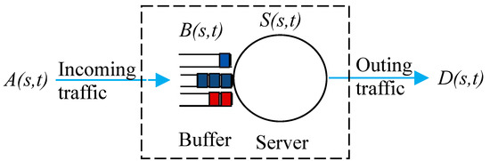
Figure 1.
Queuing model of a store forward node.
We assumed that, along with the non-decreasing (in t) bivariate processes, , and are also stationary non-negative random processes with for all . The cumulative arrival and service processes for all are given as follows:
where and are instantaneous values during the time slot.
denotes the virtual delay of the system at time t. The (min, +) algebra is the basis of network calculus, for which convolution and deconvolution play a crucial role in determining bounds on the system performance. For non-decreasing and strictly positive bivariate processes and , the (min, +) convolution and deconvolution are, respectively, defined as,
In the queueing system, we characterize time-varying systems using a dynamic server that relates the departures of a system to its arrivals as for all , which holds with strict equality when the system is linear [10]. An example of a system that satisfies the definition of a dynamic server is a lossless, work-conserving server with a time-varying capacity. Based on this server model, the end-to-end delay and PDV, which are critical performance measures in system evaluation, can be analyzed using network calculus [11].
For a given queueing system with cumulative arrival and departure and for , the virtual delay is defined as the time it takes for the last bit received by time t to leave the system under a first-come-first-serve (FCFS) scheduling scheme [12]. Therefore,
Substituting and using (min, +) convolution and the deconvolution definitions in (5), we can obtain the following bounds on [13] as
3.2. MGF-Based Network Analysis
In deterministic network calculus, the delay and PDV can be bounded in worst-case scenarios by combining traffic envelopes (upper bounds on arrivals) and service curves (lower bounds on services). The performance bounds obtained using deterministic calculus are tight for specific sample paths. Deterministic network calculus accumulates the bursts, leading to pessimistic bounds and over-utilization of resources. On the contrary, the probabilistic performance bounds obtained using stochastic network calculus provide a more realistic description of system performance than the worst-case analysis. In the probabilistic scenario where the arrival and the service process are stationary random processes, the delay bounds defined in (5) and (6) are reformulated as:
where denotes the target probabilistic delay associated with the violation probability . The performance bounds can be derived from the distributions of the processes, e.g., by using arrival and service processes’ MGFs [14]. These approaches fall into the domain of stochastic network calculus and are most suitable for the analysis of stochastic multi-hop network models [15].
MGFs of a random variable X are defined for any as
where E is the expectation of its argument. Similarly, we can derive
Using Chernoff’s bound [16], the violation probability of an effective bound x for a random variable X is given below for any x and any ,
The -traffic model shown in Figure 2 is applied to both through and cross traffic to derive closed-form solutions for end-to-end performance bounds. It is possible to describe a wide variety of traffic models using the -traffic characterization [17], including periodic, fluid, on–off, and regulated sources. An arrival process with MGF is - upper constrained for some if, for all , it holds that
where .
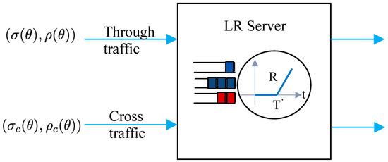
Figure 2.
Traffic model of a single node.
The service available for the through traffic and not for the cross traffic is of prime interest, and it is called the leftover service. Therefore, we estimated the amount of service capacity offered to the through traffic in the presence of the cross traffic. The MGF of the leftover service of a latency rate (LR) server with latency , capacity and cross traffic is bounded according to
where
is a latency induced by the cross traffic.
3.3. Multi-Hop Networks
The significant advantage of network calculus is that the concatenation of servers becomes easier in concatenated systems, e.g., multi-hop store-and-forward networks. Using the associativity of the (min, +) convolution, it is possible to replace servers in tandem with one system whose service curve is the (min, +) convolution of their service curves [18].
For given n tandem servers with through and cross traffic flows, as shown in Figure 3, the network service process is provided by
where , for any , represents the leftover service process of the server.
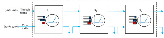
Figure 3.
Tandem servers with cross traffic.
The MGF of the end-to-end service process, written as , of n independent tandem servers, is bounded by
where ∗ is a univariate operator such that
Then, the MGF for the (min, +) deconvolution is bounded as follows:
where o is a univariate operator such that
Using these network calculus basics, we derive the delay and PDV bounds for multi-hop networks in the following section.
4. End-to-End Probabilistic Bounds in Multi-Hop Networks
An essential aspect of a network performance analysis is scaling of end-to-end delay and PDV bounds across a series of n servers. We considered the scenario shown in Figure 3, where performance bounds are derived for the through flows that traverse all n servers in series. Cross traffic joins and leaves the server at each stage.
For through traffic subjected to a series of constant-rate servers, the convolution of the MGFs of individual stages was derived in [19], and the results can be extended for LR servers.
For the single-node case:
where and for stability. This means that the average arrival rate of traffic should be less than the service rate of the server. Thus, the stability condition maintains the server utilization below a certain level.
For the multi-node (n) LR server case:
The equivalent latency for n servers can be defined as
Assuming the same latency for all servers,
The equivalent rate for n servers is given by
Using the equivalent rate, latency, and rearranging,
The probability that the delay is greater than the value d is bounded by the deconvolution of the arrival and service processes:
The MGF of can be denoted as
for all . We define another random variable, , such that
Since the random variables and are statistically ordered, their distribution is also ordered. Hence,
Thus, the first-order moments (average delay) and second-order moments (delay variance) for and are ordered. The first-order moment is given by
The probability that the delay is equal to the value d can be denoted by
Hence, the first-order moment can be obtained as
The second-order moment is given by
The second-order moment can be obtained as
The moment computation can be used to further determine the bounds for PDV.
Theorem 1
(End-to-end delay and PDV). Consider n work-conserving, latency rate servers in series, each with capacity C, latency T’, and independent cross traffic under the general scheduling model. Consider the aggregate of through flows that traverses all n servers in series. If d and v are the delay and PDV bounds with violation probability and for any such that for stability, then
The proof for this theorem is covered in Appendix A.
5. Performance Evaluation of Multi-Hop Wired Network
For the evaluation, we provide the numerical delay and PDV bounds for n servers with cross traffic in series, as shown in Figure 3. Each server has a capacity of C, and the leftover service is determined according to the general scheduling model.
A variety of arrival processes, such as voice audio sources, have been widely described using Markov models. We utilized these models to describe random processes , which represent the arrival process for cross traffic, and we were able to derive the corresponding MGFs based on these models. A typical irreducible and homogeneous Markov chain includes n states and a stationary state distribution D. During state i, the traffic workload is processed at . The discrete-time model assumes as the diagonal matrix and Q as the transition probability matrix, where is the transition probability from state i to state j [20].
It is possible to find closed-form solutions to Markov models with two states. The closed-form bounds for two-state, continuous-time models have been published for all .
Let us consider the continuous-time model, as shown in Figure 4, with two states, on and off, and represent the elements of Q by , where and . During the off state, no workload is processed. The traffic workload is processed only in the on state with the rate h and being the average rate. We have for all and all [21], such that
where, .
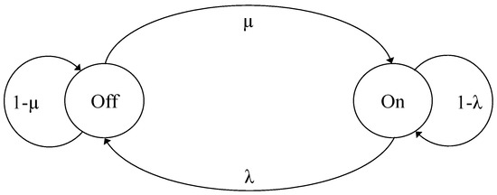
Figure 4.
Two state on–off Markov model.
For the analysis, we simulated the network using various parameters, shown in Table 1, and computed the delay and PDV bounds in the MATLAB simulator. We used a two-state Markov model to describe cross traffic with computed using (37). We completed the analysis for single- and multiple-stage networks.

Table 1.
Parameters used in the analysis.
5.1. Single-Stage Case
Figure 5 shows the results for a single server with a peak rate of cross traffic during the on state h and the off to on transition probability being maintained constant at 60 kbps and , respectively. As the on to off transition probability is varied from 0 to 1, the system shows instability up to , and after that, the delay and PDV (variance) bound curves show a decline in values. The decline is steeper in the case of PDV compared to delay. As increases, the cross traffic process tends to stay more in the off state and continuously reduces the traffic in the network. The average rate of cross traffic reduces with an increase in , raising the peak-to-average rate with it. This means that less bursty cross traffic is experienced by through traffic flows. This network behavior causes the delay and PDV bound curves to experience a decline. The PDV expression in (A14) indicates that the part of the PDV bound depends on the changes in the average rate of cross traffic, and hence, its decline is steeper. The practical range of for the PDV bound control is greater than 0.43 for this configuration. The values below 0.43 indicate unstable conditions when the average rate is the same or closer to the peak rate.
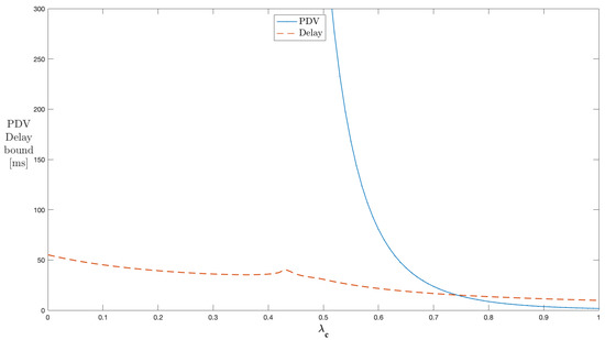
Figure 5.
Impact of on the PDV bound in a single-stage network (constant ).
Similarly, Figure 6 shows the results for a single server if the off to on transition probability is varied from 0 to 1. The peak rate of cross traffic during the on state h and the on to off transition probability are kept constant at 60 kbps and , respectively. With the increase in , the traffic in the network continuously increases, resulting in delay and PDV bound curves experiencing a rise; however, this rise is sharper for PDV compared to its delay counterpart. As increases, the cross traffic process tends to stay more in the on state and continuously increases the traffic in a network. The average rate of cross traffic increases with the rise in . Thus, the peak-to-average rate increases with it. This means that more bursty cross traffic is experienced by through traffic flows. This network behavior causes the delay and PDV bound curves to experience a rise. The PDV bound expression in (A14) indicates that the part of PDV depends up the changes in the average rate of cross traffic, whereas the delay bound comprises the latency due to the burst size of the through flows and the latency of the server induced by cross traffic. Thus, lowering the average rate makes PDV rise steeper. All the range of the values can be used to control the PDV bounds for this configuration.
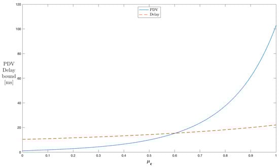
Figure 6.
Impact of on the PDV bound in a single-stage network (constant ).
5.2. Multi-Stage Case
Figure 7 shows the results for to 10 servers with through and cross traffic in series. The parameters used were and , and the peak rate kbps was chosen. The system is unstable up to . The instability indicates that the average rate is the same or closer to the peak rate during this time. After that, with the addition of each server to the network topology, the delay and PDV bounds show an increase in values. The results confirm the scalability of the performance bounds. The same traffic continues through a series of network servers, and thus, the burstiness due to a change in the average rate is accumulated with each new server and subjected to the subsequent stage. Thus, the PDV bound shows a steeper rise with the addition of servers compared to delay. The increment in the end-to-end delay and the PDV bound for each additional concatenated server is greater than the bound that would be obtained for the server in isolation.
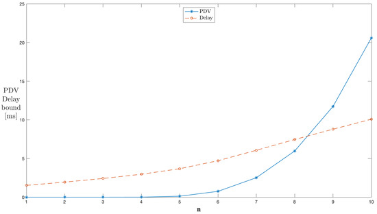
Figure 7.
End-to-end concatenation of servers in series.
Figure 8 shows the results of the delay and PDV bound curves for to 10 servers with the peak rate h and , kept constant at 60 kbps and , respectively. With increasing from 0 to 1, the delay and PDV bound curves corresponding to the number of servers (1 to 10) follow the decrement pattern in values identical to that of the single stage. With increasing the number of servers, the PDV bound curve shifts to the right, indicating a late starting point on the scale, but higher values after the start compared to the previous curve. This means that, as we continue to increase the number of stages, the PDV and delay bound values reach higher than the previous number of stages, which is true for all the range of values. The operating region of the values for managing PDV reduces as we continue to increase the number of stages.
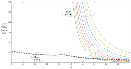
Figure 8.
Impact of n and on the PDV bound in a multi-stage network (constant ).
Figure 9 shows the results of the delay and PDV bound curves for to 10 servers with the peak rate h and , kept constant at 60 and , respectively. The parameter was varied from 0 to 1. The delay and PDV bound curves follow the same increment pattern as for the single stage; also, the increase is steeper for PDV than delay as observed with the single-stage case. As the number of servers increases, the PDV bound curves start at a lower value and show small value increases compared to previous server configurations. This means that, as we continue to increase the number of stages, the PDV and delay bounds reach lower values for the previous number of stages, which is true for all the range of values. The useful region of values for managing the PDV bound reduces as we continue to increase the number of stages.
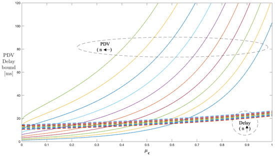
Figure 9.
Impact of n and on the PDV bound in a multi-stage network (constant ).
5.3. Discussion
The stable operating regions of analysis can be obtained by checking the performance of PDV against various burstiness levels of cross traffic. We used the parameters from Table 1 for this analysis. The peak-to-average ratio of cross traffic indicates the burstiness level of cross traffic. Figure 10 shows the impact of the peak-to-average rate ratio of cross traffic on the PDV and delay bounds when is kept constant at 0.7. The valid PDV bound values start when the peak-to-average rate reaches . Beyond , the PDV bounds decrease exponentially with the peak-to-average rates. The valid values start from . Thus, the unstable region for this configuration is when the peak-to-average rate is less than , which corresponds to the values being less than . Similarly, Figure 11 shows the impact of the peak-to-average rate ratio of cross traffic on the PDV and delay bounds when is kept constant at 0.7. The valid PDV bound values start when the peak-to-average rate reaches . Beyond , the PDV bounds decrease exponentially with the peak-to-average rates. All the values can lead to valid PDV values. Thus, the unstable region for this configuration is when the peak-to-average rate is less than .
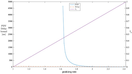
Figure 10.
Impact of the peak-to-average rate ratio of cross traffic on the PDV bound in a single-stage network (constant ).
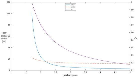
Figure 11.
Impact of the peak-to-average rate ratio of cross traffic on the PDV bound in a single-stage network (constant ).
The PDV performance was evaluated in different network conditions to cover the corner cases. The different network scenarios were created by varying the burstiness of cross traffic. The approach of varying cross traffic dynamics using different peak-to-average rates of cross traffic was discussed in [22]. This, in turn, can be achieved by changing the transition probabilities and from the minimum to the maximum limits. To further strengthen the confidence in the analysis, we simulated the through traffic in the presence of cross traffic in the time domain using the parameters listed in Table 2. The cross traffic was generated with the average rate of 35 kbps using the Markovian process. For a seven-stage network, the PDV output is shown in Figure 12. The average PDV bound value of 1.6 ms seems practical for the given configuration.
Table 2.
Parameters used in time simulation.
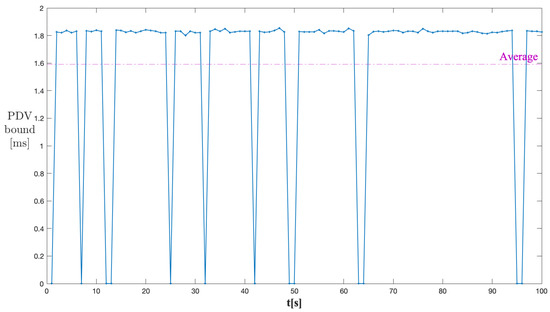
Figure 12.
PDV bound output for through traffic (time simulation).
Overall, the analysis revealed the behavior of PDV bounds under different network conditions influenced by cross traffic parameters. For a single stage, the upper bound of the PDV changes from 276 ms to 7 ms when increases from to , keeping constant at . Similarly, the upper bound of PDV for a single stage varies from 4 ms to 64 ms when increases from to , keeping constant at . For a seven-stage configuration, the upper bound of PDV changes from 274 ms to 40 ms when increases from to , keeping constant at . Similarly, the upper bound of PDV for a seven-stage configuration varies from 15 ms to 97 ms when increases from to , keeping constant at . Thus, the PDV observations from single- and multi-stage configurations proved the initial hypothesis. When changed in a planned manner, the traffic parameters can control the range in which the PDV can vary. This is an important observation as there are many applications where keeping the PDV under control or within a prescribed range can result in maintaining the QoS for the traffic of interest. A background traffic shaper can be conceived of based on the dependence of the PDV on the traffic parameters. The analysis showed promising results in maintaining the QoS in the presence of unpredictable background traffic using such a shaper.
The known limitations of this approach are as follows. The background traffic was assumed to be not as critical as the traffic of interest or real-time traffic. Better PDV performance was achieved at the cost of slightly degraded background traffic performance. It is possible that the background traffic would take more than usual to reach its destination than in the typical case. Secondly, the approach is feasible only under stable conditions, as defined above. Thirdly, the stochastic network calculus provided the bounds on delay and PDV with a certain violation probability, and practical translation of these results must take into account all the assumptions and uncertainties.
6. Conclusions
Ensuring network QoS for real-time services in industrial and other domains is essential to meet the strict deadlines of real-time applications. Jitter or PDV is a crucial performance indicator for real-time applications in a communication network. The real-life performance of PDV depends on ever-changing background traffic due to the introduction of new devices, services, and applications to the communication network. We utilized network calculus toolboxes such as moment-generating functions and (min, +) algebra to study and investigate delay and PDV in a wired packet switched network. We derived an analytic expression for evaluating end-to-end delay and jitter bounds incurred by a traffic of interest by the presence of background traffic. The analysis based on simulations confirmed the scalability of the PDV expression with an increasing number of servers in a multi-hop network. The PDV analysis conducted with the help of the Markovian traffic model for background traffic showed that the background traffic parameters can significantly affect the end-to-end PDV bound. The analysis showed promising results to conceive of a traffic shaper for background traffic using the Markovian models. The end-to-end PDV can be controlled by changing the settings of the network model parameters. Thus, the gained knowledge can be utilized to shape background traffic to achieve the desired QoS performance required for real-time applications.
PDV is significant in deciding the performance of many network-based applications. Bounding the PDV or jitter under a certain level can be beneficial for such applications. The next step within our work could be to assess the feasibility of employing the results of the PDV analysis in applications where the PDV needs to be bounded. Further, the possibility of designing a background network traffic filter can be investigated for such applications.
Author Contributions
Conceptualization, R.N.G., E.L., J.Å. and M.B.; funding acquisition, J.Å. and M.B.; investigation, R.N.G., E.L., J.Å. and M.B.; methodology, M.B.; project administration, J.Å.; supervision, E.L., J.Å. and M.B.; writing—original draft, R.N.G.; writing—review and editing, R.N.G., E.L., J.Å. and M B. All authors have read and agreed to the published version of the manuscript.
Funding
This work was financed by the Future Industrial Networks (FIN) project, Grant Number 2018-02196, within the strategic innovation program for process industrial IT and automation, PiiA, and PiiA Research Etapp II, a joint program by Vinnova, Formas, and Energimyndigheten.
Conflicts of Interest
The authors declare no conflict of interest.
Appendix A. Proof for Theorem 1
The end-to-end delay bound is violated at most with probability if, for any , it holds that
Inserting (21) into (A1),
The expression for d can be obtained by simplifying (A2).
References
- Jia, P.; Wang, X.; Shen, X. Digital Twin Enabled Intelligent Distributed Clock Synchronization in Industrial IoT Systems. IEEE Internet Things J. 2020, 8, 4548–4559. [Google Scholar] [CrossRef]
- Toral-Cruz, H.; Pathan, A.S.; Ramirez-Pacheco, J. Accurate modeling of VoIP traffic QoS parameters in current and future networks with multifractal and Markov models. Math. Comput. Model. 2013, 57, 2832–2845. [Google Scholar] [CrossRef]
- Brun, O.; Bockstal, C.; Garcia, J. A Simple Formula for End-to-End Jitter Estimation in Packet-Switching Networks. In Proceedings of the International Conference on Networking, International Conference on Systems and International Conference on Mobile Communications and Learning Technologies 2006, Morne, Mauritius, 23–29 April 2006; p. 14. [Google Scholar]
- Matragi, W.; Sohraby, K.; Bisdikian, C. Jitter calculus in ATM networks: Multiple nodes. IEEE/ACM Trans. Netw. 1997, 5, 122–133. [Google Scholar] [CrossRef]
- Dahmouni, H.; Girard, A.; Sanso, B. An analytical model for jitter in IP networks. Annales Télécommunications 2012, 67, 81–90. [Google Scholar] [CrossRef]
- Dbira, H.; Girard, A.; Sanso, B. Calculation of packet jitter for non-poisson traffic. Ann. Telecommun. 2016, 71, 223–237. [Google Scholar] [CrossRef]
- Geleji, G.; Perros, H. Jitter analysis of an MMPP-2 tagged stream in the presence of an MMPP-2 background stream. Appl. Math. Model. 2014, 38, 3380–3400. [Google Scholar] [CrossRef]
- Thombre, S. Network Jitter Analysis with varying TCP for Internet Communications. In Proceedings of the 3rd International Conference for Convergence in Technology (I2CT) 2018, Pune, India, 6–8 April 2018; pp. 1–7. [Google Scholar]
- Fei, N.; Xuefen, C.; Wen, D.; Haifeng, Y. Jitter analysis of real-time services in IEEE 802.15.4 WSNs and wired IP concatenated networks. J. China Univ. Posts Telecommun. 2016, 23, 1–8. [Google Scholar] [CrossRef]
- Yang, G.; Xiao, M.; Al-Zubaidy, H.; Huang, Y.; Gross, J. Analysis of Millimeter-Wave Multi-Hop Networks With Full-Duplex Buffered Relays. IEEE/ACM Trans. Netw. 2018, 26, 576–590. [Google Scholar] [CrossRef]
- Azuaje, O.; Aguiar, A. End-to-End Delay Analysis of a Wireless Sensor Network Using Stochastic Network Calculus. In Proceedings of the Wireless Days (WD), Manchester, UK, 24–26 April 2019; pp. 1–8. [Google Scholar]
- Al-Zubaidy, H.; Liebeherr, J.; Burchard, A. A (min, ×) network calculus for multi-hop fading channels. In Proceedings of the IEEE INFOCOM 2013, Turin, Italy, 14–19 April 2013; pp. 1833–1841. [Google Scholar]
- Miao, W.; Min, G.; Wu, Y.; Huang, H.; Zhao, Z.; Wang, H.; Luo, C. Stochastic Performance Analysis of Network Function Virtualization in Future Internet. IEEE J. Sel. Areas Commun. 2019, 37, 613–626. [Google Scholar] [CrossRef]
- Nikolaus, P.; Schmitt, J. Improving Output Bounds in the Stochastic Network Calculus Using Lyapunov’s Inequality. In Proceedings of the IFIP Networking Conference (IFIP Networking) and Workshops, Zurich, Switzerland, 14–16 May 2018; pp. 1–9. [Google Scholar]
- Petreska, N.; Al-Zubaidy, H.; Knorr, R.; Gross, J. On the recursive nature of end-to-end delay bound for heterogeneous wireless networks. In Proceedings of the IEEE International Conference on Communications (ICC), London, UK, 8–12 June 2015; pp. 5998–6004. [Google Scholar]
- Mulzer, W. Five Proofs of Chernoff’s Bound with Applications. arXiv 2018, arXiv:1801.03365. [Google Scholar]
- Liu, Y. Stochastic Network Calculus. In Stochastic Network Calculus; Springer: London, UK, 2009; ISBN 978-1-84800-127-5. [Google Scholar]
- Fidler, M.; Rizk, A. A Guide to the Stochastic Network Calculus. IEEE Commun. Surv. Tutor. 2015, 17, 92–105. [Google Scholar] [CrossRef]
- Fidler, M. An End-to-End Probabilistic Network Calculus with Moment Generating Functions. In Proceedings of the 14th IEEE International Workshop on Quality of Service, New Haven, CT, USA, 19–21 June 2006; pp. 261–270. [Google Scholar]
- Fidler, M. WLC15-2: A Network Calculus Approach to Probabilistic Quality of Service Analysis of Fading Channels. In Proceedings of the IEEE Globecom 2006, San Francisco, CA, USA, 27 November–1 December 2006; pp. 1–6. [Google Scholar]
- Courcoubetis, C.; Weber, R. Buffer Overflow Asymptotics for a Buffer Handling Many Traffic Sources. J. Appl. Probab. 1996, 33, 886–903. [Google Scholar] [CrossRef]
- Al-Zubaidy, H.; Liebeherr, J.; Burchard, A. Network-Layer Performance Analysis of Multihop Fading Channels. IEEE/ACM Trans. Netw. 2016, 24, 204–217. [Google Scholar] [CrossRef]


Publisher’s Note: MDPI stays neutral with regard to jurisdictional claims in published maps and institutional affiliations. |
© 2022 by the authors. Licensee MDPI, Basel, Switzerland. This article is an open access article distributed under the terms and conditions of the Creative Commons Attribution (CC BY) license (https://creativecommons.org/licenses/by/4.0/).