Article

Model-Free Adaptive Control Based on Fractional Input-Output Data Model

by
Chidentree Treestayapun
1,† and
Aldo Jonathan Muñoz-Vázquez
2,*,†
1
Department of Robotics and Advanced Manufacturing, Center for Research and Advanced Studies (CINVESTAV), Saltillo Campus, Saltillo 25900, Coahuila, Mexico
2
Department of Multidisciplinary Engineering, Higher Education Center at McAllen, Texas A&M University, McAllen, TX 78504, USA
*
Author to whom correspondence should be addressed.
These authors contributed equally to this work.
Appl. Sci. 2022, 12(21), 11168; https://doi.org/10.3390/app122111168
Submission received: 3 September 2022 / Revised: 28 October 2022 / Accepted: 2 November 2022 / Published: 4 November 2022

Abstract

:
Memory properties of fractional-order operators are considered for an input-output data model for highly uncertain nonlinear systems. The model arises by relating the fractional-order variation of the output to the fractional-order variation of the input; the instantaneous gain is computed through a fuzzy inference network, whose output consequences are adapted online on a gradient descent rule. The fractional-order nature of the proposed model relaxes the stringent conditions on data-driven schemes, allowing instantaneous changes in the output signal with a null variation in the controller. The main contribution consists of taking advantage of the memory properties of fractional-order operators and the flexibility of fuzzy logic rules to construct a data-driven model for highly uncertain discrete-time nonlinear systems. The relevance of the proposed method is assessed through experiments in a real-world scenario.

1. Introduction

Robust tracking and regulation in highly uncertain discrete-time nonlinear systems is a non-trivial and interesting problem. This paper proposes a fractional input-output data model that relies on a dynamic linearization between the fractional-order variation of the input function and the fractional-order variation of the output signal, in contrast to classical approaches that consider just local information related to first-order variations [1]. An intrinsic advantage of the proposed method is that the model is still valid when there are instantaneous changes in the output signal, while the variation in the controller is null. Another advantage is less sensitivity to measurement and input noise because more data are considered to synthesize the equivalent model. These features can be provided by the inherent memory properties of fractional-order operators [2,3,4,5].
Modern engineering systems are composed of different elements with uncertain models. This motivates the study of model-free approaches that rely on less restrictive assumptions on the system response [6,7,8]. In addition, computing the controller during the implementation time is of preponderant importance to assure a good degree of robustness and performance [9].
In recent years, the paradigm of data-driven control has been considered for the case of complex and uncertain dynamic systems [10,11,12,13,14]. In particular, the concept of compact form dynamic linearization was investigated in [9], which proposed a data-driven model that relates the first-order variations of input and output signals by means of an instantaneous gain, also called the pseudo-partial derivative (PPD). The validity of the proposed model relies on assuring that the PPD is finite for any time instant, thus, the equivalent model is undefined if there is any variation of the output but the input remains at a constant value.
In order to estimate the PPD, a fuzzy logic formulation was proposed in [15], where the universal approximation properties of fuzzy systems are considered to compute the equivalent model. Full and partial forms of dynamic linearizations were investigated in [16,17], accounting for more data to produce a more accurate model representation. Nevertheless, this was done at the price of adjusting more parameters.
A popular scheme for model-free implementation is, for instance, the proportional-integral-derivative (PID) control, which is very appealing in industrial applications due to its simplicity and reliability [18,19]. In addition, the increasing in complexity of modern automation applications requires more robust and more flexible techniques to operate in uncertain conditions, thus, some advanced versions of the PID control consider sliding mode [20,21], fractional-order [22], fuzzy logic [23], and adaptive schemes [24]. However, a structure for the dynamical model is still necessary to assure, at least analytically, an acceptable closed-loop response.
In this paper, the inherent memory properties of fractional-order operators [25,26] are considered to produce a discrete-time equivalent input-output data model, where the fractional PPD (FPPD) is computed by means of fuzzy rules emulating networks. The advantages of the proposed scheme consist of accounting for the history of the process, while searching for a single parameter through a fuzzy aggregation scheme. An interesting property of the proposed algorithm is that the model is still valid when the output changes in the presence of a locally constant output signal.
It is important to note that some neural network structures can be considered [27,28,29], as an alternative to the fuzzy logic approach, to actively estimate the FPPD during implementation time. Nonetheless, the user experience on the system behaviors can be of great value when designing the fuzzy inference system [30,31].
The remaining of this paper is organized as follows. The next section presents the problem formulation. The fractional input-output equivalent model is presented in Section 3. The control design is given in Section 4. The experimental results are analyzed in Section 5, and the main conclusions are discussed in Section 6.

2. Problem Formulation

Consider a class of discrete-time nonlinear systems of the form
y ( k + 1 ) = f ( y ¯ ( k ) , u ¯ ( k ) ) ,
where f ( ) is an unknown, but smooth, nonlinear function, y ( k + 1 ) R is the output, and u ( k ) R is the control input. Consider the vectors y ¯ ( k ) = [ y ( k ) , y ( k 1 ) , , y ( k n y ) ] T and u ¯ ( k ) = [ u ( k ) , u ( k 1 ) , , u ( k n u ) ] T , where n y and n u are unknown integer numbers.
The problem is to design u ( k ) , such that the output y ( k ) tracks a smooth desired reference r ( k ) . Moreover, only input-output data are available for control purposes, that is, y ( k ) and u ( k ) , and their preceding values.

3. Fractional Input-Output Equivalent Model

The discrete-time fractional difference of the sequence x ( k ) R , with  k N 0 , is defined as
Δ N α x ( k ) = i = 0 N ω α ( i ) x ( k i ) ,
where α ( 0 , 1 ] is the order, and the fractional binomial coefficient ω α ( i ) is determined recursively as
ω α ( i ) = 1 1 + α i ω α ( i 1 ) ,
for i 1 , and initial condition ω α ( 0 ) = 1 .
Accordingly, the equivalent model based on the FPPD (fractional pseudo partial derivative) θ ( k ) is proposed as
Δ N y α y ( k + 1 ) = θ ( k ) Δ N u α u ( k ) .
Relying on the definition in (2), we have
Δ N y α y ( k + 1 ) = ω α ( 0 ) y ( k + 1 ) + + ω α ( N y ) y ( k N y + 1 ) ,
and
Δ N u α u ( k ) = ω α ( 0 ) u ( k ) + + ω α ( N u ) u ( k N u ) .
Simplifying ω ( i ) = ω α ( i ) and using (3), we obtain
y ( k + 1 ) = θ ( k ) Δ N u α u ( k ) ω ( 1 ) y ( k ) ω ( 2 ) y ( k 1 ) ω ( N y ) y ( k N y + 1 ) .
Therefore, the equivalent model is formulated as
y ^ ( k + 1 ) = θ ^ ( k ) Δ N u α u ( k ) ω ( 1 ) y ( k ) ω ( 2 ) y ( k 1 ) ω ( N y ) y ( k N y + 1 ) ,
where y ^ ( k + 1 ) is the output of the equivalent model and θ ^ ( k ) is the estimated FPPD. With the aim of utilizing the fractional input-output equivalent model proposed by (8), the adaptive network multiple-input fuzzy rules emulating network (MiFREN) is employed to establish θ ^ ( k ) .
The fuzzy network architecture relies on the IF-THEN rules:
  • ∘ Rule i = 1 , , N f :
  • {IF u ( k 1 ) is μ u i and y ( k ) is μ y i THEN θ ^ i ( k ) = β i ( k ) },
where N f is the number of IF-THEN rules, μ u i and μ y i are membership functions of u ( k 1 ) and y ( k ) , respectively, and  β ( k ) R N f is the weight-vector of output consequences. In addition, considering φ i ( k ) = μ u i μ y i , with the product as the t-norm, as the degree of validity of Rule i . Then, the estimated FPPD, or  θ ^ ( k ) , is obtained as
θ ^ ( k ) = i = 1 N f φ i ( k ) β i ( k ) = φ T ( k ) β ( k ) .
An alternative for the membership functions is given by
  • x is POSITIVE: μ P ( x ) = 0.5 [ 1 + tanh ( σ x 1 ) ] ;
  • x is ZERO: μ N ( x ) = 1 tanh 2 ( σ x ) ; and
  • x is NEGATIVE μ Z ( x ) = 0.5 [ 1 tanh ( σ x + 1 ) ] ,
for agglomeration parameter σ > 0 . Note that, if the range of argument x is small, the parameter σ should be large, and vice-versa. Moreover, the adaptation allows us to reduce the number of fuzzy sets, and in turns the number of rules, to be considered.
The learning law of the weight parameters β ( k ) in (9) is derived from minimizing the cost function
E ^ ( k + 1 ) = 1 2 e ^ 2 ( k + 1 ) ,
where e ^ ( k + 1 ) is the model error given by
e ^ ( k + 1 ) = y ( k + 1 ) y ^ ( k + 1 ) .
By employing the gradient descent approach to minimize the cost function (10), the learning law for β ( k + 1 ) is derived as
β ( k + 1 ) = β ( k ) η ( k ) E ^ ( k + 1 ) β ( k ) T ,
where η > 0 is the learning rate. Applying the chain rule with (10) through (9) and (8), E ^ ( k + 1 ) β ( k ) in (12) can be obtained as
E ^ ( k + 1 ) β ( k ) = E ^ ( k + 1 ) e ^ ( k + 1 ) e ^ ( k + 1 ) y ^ ( k + 1 ) y ^ ( k + 1 ) θ ^ ( k ) θ ^ ( k ) β ( k ) , = e ^ ( k + 1 ) Δ N u α u ( k ) φ T ( k ) .
Substitution of (13) into (12) leads to the learning law
β ( k + 1 ) = β ( k ) + η e ^ ( k + 1 ) Δ N u α u ( k ) φ ( k ) .
Furthermore, the appropriate learning rate η is established by the following result to guarantee an acceptable performance of the equivalent model.
Lemma 1.
Consider the fractional-order dynamics in (5), whose equivalent model is given in (8) and (9). Then, the boundedness of the internal signals and the model error is guaranteed if the learning rate η is selected with a positive constant μ η as
η = γ η μ η + Δ u M 2 φ M 2 ,
where
0 < γ η < 1 ,
φ M | | φ ( k ) | | ,
and
Δ u M | Δ N u α u ( k ) | .
Proof. 
According to the universal approximation property of the MiFREN method [32], with the estimated FPPD in (9), and the ideal weight vector β * , one has that θ ( k ) in (9) can be rewritten as
θ ( k ) = φ T ( k ) β * + ε θ ( k ) ,
where | ε θ ( k ) | ε θ M is the bounded residue error.
By using (19) with (7), one gets
y ( k + 1 ) = [ φ T ( k ) β * + ε θ ( k ) ] Δ N u α u ( k ) ω ( 1 ) y ( k ) ω ( 2 ) y ( k 1 ) ω ( N y ) y ( k N y + 1 ) = y Δ N y ( k ) + φ T ( k ) β * Δ N u α u ( k ) + ε θ ( k ) Δ N u α u ( k ) ,
where
y Δ N y ( k ) = ω ( 1 ) y ( k ) + ω ( 2 ) y ( k 1 ) + + ω ( N y ) y ( k N y + 1 ) .
Next, using (8) and (9) produces
y ^ ( k + 1 ) = y Δ N y ( k ) + φ T ( k ) β ( k ) Δ N u α u ( k ) .
By utilizing the model error (11) with (20) and (22) yields
e ^ ( k + 1 ) = y ( k + 1 ) y ^ ( k + 1 ) = φ T ( k ) [ β * β ( k ) ] Δ N u α u ( k ) + ε θ ( k ) Δ N u α u ( k ) = φ T ( k ) β ˜ ( k ) Δ N u α u ( k ) + ε θ ( k ) Δ N u α u ( k ) ,
where
β ˜ ( k ) = β * β ( k ) .
Applying one-step forward with (24) and using (14) leads to
β ˜ ( k + 1 ) = η e ^ ( k + 1 ) Δ N u α u ( k ) φ ( k ) + β ˜ ( k ) , = η [ φ T ( k ) β ˜ ( k ) Δ N u α u ( k ) + ε θ ( k ) Δ N u α u ( k ) ] Δ N u α u ( k ) φ ( k ) + β ˜ ( k ) = I η | Δ N u α u ( k ) | 2 φ ( k ) φ T ( k ) β ˜ ( k ) η ε θ ( k ) | Δ N u α u ( k ) | 2 φ ( k ) .
Note that, for β ( k ) φ ( k ) , one has that β ( k ) T φ ( k ) = β * φ ( k ) . Thereby, only the case of β ( k ) φ ( k ) is considered, and consequently,
β ˜ ( k + 1 ) = 1 η | Δ N u α u ( k ) | 2 | | φ ( k ) | | 2 β ˜ ( k ) η ε θ ( k ) | Δ N u α u ( k ) | 2 φ ( k ) .
Therefore, the learning rate η in (15) renders
0 < 1 η | Δ N u α u ( k ) | 2 | | φ ( k ) | | 2 < 1 .
Thus, β ˜ ( k ) is a bounded sequence for a control effort u ( k ) with bounded fractional difference Δ N u α u ( k ) . Thereafter, the model error e ^ ( k ) is also a bounded sequence according to (23) and the boundedness of β ˜ ( k ) . □

4. Adaptive Controller

By utilizing the fractional equivalent model proposed in (8), the adaptive control law is derived in this section. First, the filtered tracking error s ( k ) is defined as
s ( k ) = e ( k ) + γ e e ( k 1 ) ,
where γ e < 1 is a parameter of design, and e ( k ) = r ( k ) y ( k ) is the tracking error for the smooth reference r ( k ) . The reaching condition is designed as
s ( k + 1 ) = γ s s ( k ) ,
where the constant parameter γ s < 1 is the reaching rate. Combining (28) and (29) results in
e ( k + 1 ) = γ s s ( k ) γ e e ( k ) .
The dynamics in (7) can be rewritten as
y ( k + 1 ) = θ ( k ) [ u ( k ) + u Δ N u ( k 1 ) ] y Δ N y ( k ) ,
where
u Δ N u ( k 1 ) = ω ( 1 ) u ( k 1 ) + + ω ( N u ) u ( k N u ) .
Thus, the error dynamics in (30) can be processed as
r ( k + 1 ) y ( k + 1 ) = γ s s ( k ) γ e e ( k ) ,
or
y ( k + 1 ) = r ( k + 1 ) + γ s s ( k ) + γ e e ( k ) ,
and consequently
r ( k + 1 ) + γ s s ( k ) + γ e e ( k ) = θ ( k ) [ u ( k ) + u Δ N u ( k 1 ) ] y Δ N y ( k ) .
Rearranging (35), the ideal control law u * ( k ) can be obtained as
u * ( k ) = 1 θ ( k ) r ( k + 1 ) + γ s s ( k ) + γ e e ( k ) + y Δ N y ( k ) u Δ N u ( k 1 ) .
Nevertheless, since θ ( k ) is unknown, the control law u ( k ) is established by θ ^ ( k ) in (9) as
u ( k ) = 1 θ ^ ( k ) + ε θ sign θ ^ ( k ) r ( k + 1 ) + γ s s ( k ) + γ e e ( k ) + y Δ N y ( k ) u Δ N u ( k 1 ) ,
where ε θ is a positive constant.
Theorem 1.
The sliding surface s ( k ) and the tracking error e ( k ) remain as bounded sequences for small enough positive gains γ s and γ e ( 0 , 1 ) .
Proof. 
Dynamics (31) with control law (37) leads to
y ( k + 1 ) = θ ( k ) { 1 θ ^ ( k ) + ε θ sign θ ^ ( k ) [ r ( k + 1 ) + γ s s ( k ) + γ e e ( k ) + y Δ N y ( k ) ] u Δ N u ( k 1 ) + u Δ N u ( k 1 ) } y Δ N y ( k ) = θ ( k ) θ ^ ε ( k ) r ( k + 1 ) + γ s θ ( k ) θ ^ ε ( k ) s ( k ) + γ e θ ( k ) θ ^ ε ( k ) e ( k ) + θ ( k ) θ ^ ε ( k ) 1 y Δ N y ( k ) ,
where
θ ^ ε ( k ) = θ ^ ( k ) + ε θ sign θ ^ ( k ) .
Thereafter, the tracking error is derived as
e ( k + 1 ) = r ( k + 1 ) y ( k + 1 ) = 1 θ ( k ) θ ^ ε ( k ) r ( k + 1 ) γ s θ ( k ) θ ^ ε ( k ) s ( k ) γ e θ ( k ) θ ^ ε ( k ) e ( k ) θ ( k ) θ ^ ε ( k ) 1 y Δ N y ( k ) .
Referring to the definition of s ( k ) in (28), one obtains
s ( k + 1 ) = e ( k + 1 ) + γ e e ( k ) = 1 θ ( k ) θ ^ ε ( k ) r ( k + 1 ) γ s θ ( k ) θ ^ ε ( k ) s ( k ) + 1 θ ( k ) θ ^ ε ( k ) γ e e ( k ) θ ( k ) θ ^ ε ( k ) 1 y Δ N y ( k ) .
In addition, consider
ξ r ( k ) = 1 θ ( k ) θ ^ ε ( k ) r ( k ) ,
ξ y ( k ) = 1 θ ( k ) θ ^ ε ( k ) y Δ N y ( k ) ,
and
ξ θ ( k ) = θ ( k ) θ ^ ε ( k ) .
Thus, the dynamics in (40) and (41) can be rearranged as
e ( k + 1 ) = γ s ξ θ ( k ) s ( k ) + γ e ξ θ ( k ) e ( k ) + ξ r ( k ) + ξ y ( k ) ,
and
s ( k + 1 ) = γ s ξ θ ( k ) s ( k ) + γ e [ 1 + ξ θ ( k ) ] e ( k ) + ξ r ( k ) + ξ y ( k ) ,
respectively. In view of (45) and (46), one obtains the closed-loop dynamics
s ( k + 1 ) e ( k + 1 ) = A 1 , 1 ( k ) A 1 , 2 ( k ) A 2 , 1 ( k ) A 2 , 2 ( k ) A θ s ( k ) e ( k ) + 1 1 [ ξ r ( k ) + ξ y ( k ) ] ,
where
A 1 , 1 ( k ) = γ s ξ θ ( k ) ,
A 1 , 2 ( k ) = γ e [ 1 + ξ θ ( k ) ] ,
A 2 , 1 ( k ) = A 1 , 1 ( k ) ,
and
A 2 , 2 ( k ) = γ e ξ θ ( k ) .
Note that ξ θ ( k ) is a bounded sequence; then, it is possible to find small enough values γ ¯ e and γ ¯ s , such that A θ is a convergent matrix, whenever 0 < γ e < γ ¯ e and 0 < γ s < γ ¯ s . One way to determine conservative bounds for γ ¯ e and γ ¯ s relies on utilizing the Gershgorin Circle Theorem, which states that all the proper values of A θ lie inside of at least one of the circles of Gershgorin. In addition, these circles are centered at A 1 , 1 and A 2 , 2 , and have radii | A 1 , 2 | and | A 2 , 1 | , respectively. Then, it suffices to show that
γ s ξ θ M + γ e ( 1 + ξ θ M ) < 1 , γ s ξ θ M + γ e ξ θ M < 1 ,
for | ξ θ ( k ) | ξ θ M . Then, the two circles are inside the unit disk if
0 < γ s , γ e < 1 2 ( 1 + ξ θ M ) .
In that case, the proper values of A θ lie inside the unit disk for any k 0 , and in particular for k . □

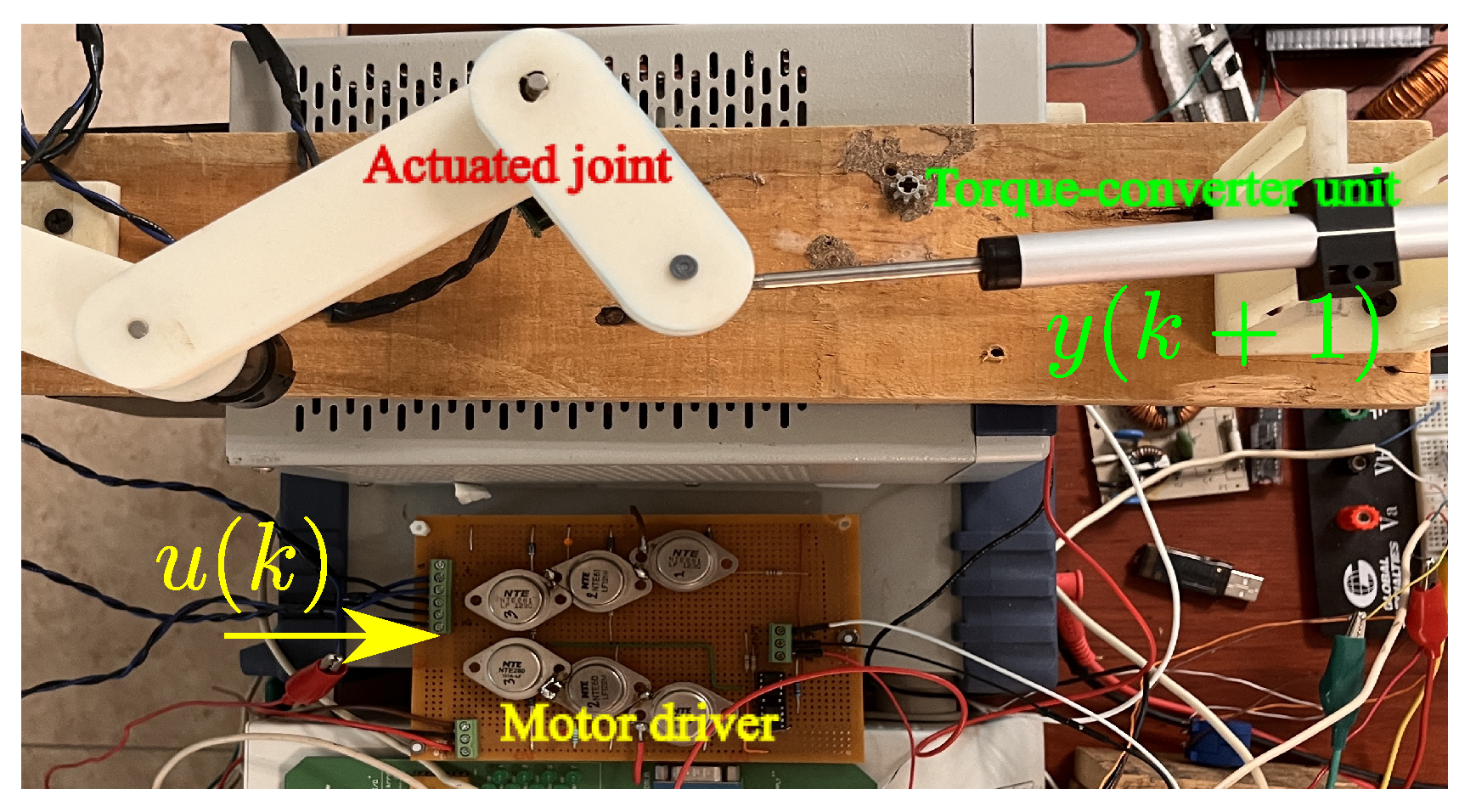
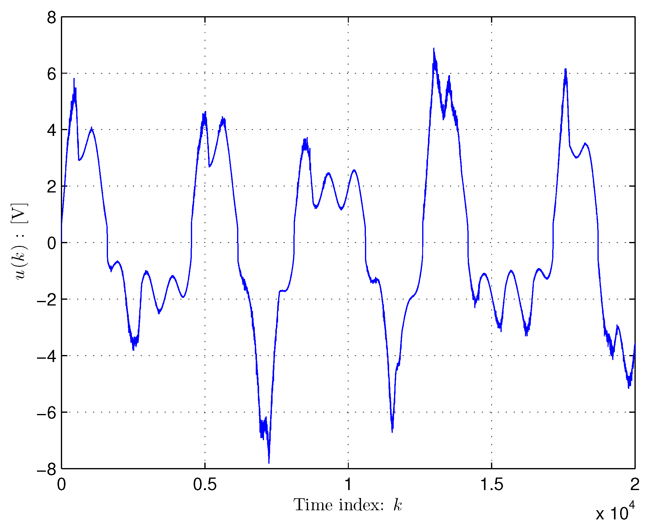
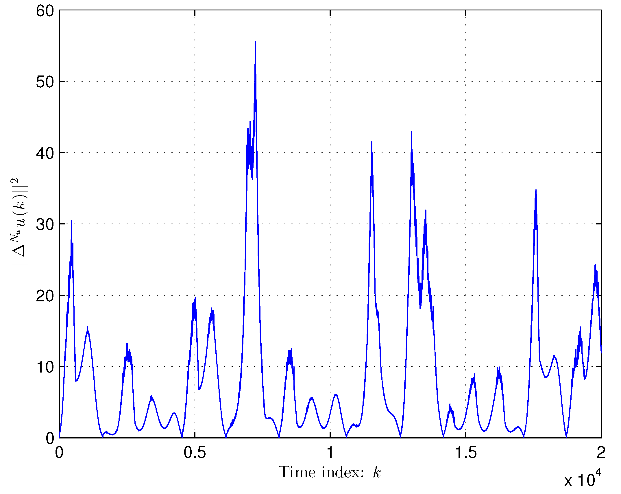
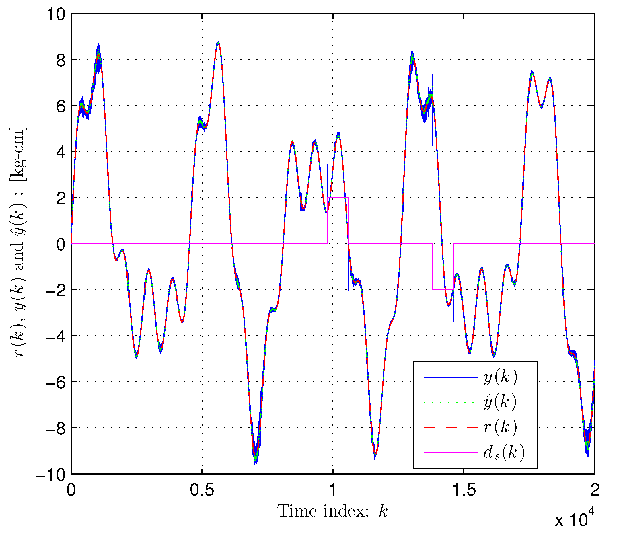
5. Experimental System and Results

To validate the performance of the proposed controller, the direct-current motor torque control system is constructed, as shown in Figure 1. A high-gain Namiki 22CL-3501PG motor is driven by push–pull transistors through the input voltage u ( k ) [V], which is generated by the analog output of CONTEC AIO-160802LPE. The output y ( k + 1 ) [kg·cm] is measured by the torque-converter that is equipped with the analog-input.
The system is considered as an unknown discrete-time nonlinear system, and only input-output data are considered to be available. Thereafter, the membership functions of y ( k ) ± 10 [kg-cm] and | u ( k 1 ) | 8 [V] are designed according to the operating ranges depicted in Figure 2.
Figure 3 shows the tracking performance with the plots of the output y ( k ) and the desired trajectory r ( k ) . Furthermore, the plot of y ^ ( k ) is provided in the same figure to demonstrate the reliability of the equivalent model. The control voltage u ( k ) is illustrated in Figure 4. The time-varying behavior of | Δ N u α u ( k ) | 2 is shown in Figure 5, which shows condition (18) using Lemma 1.
The experimental study is repeated by introducing the unknown disturbance d s ( k ) . Figure 6 shows the plots of y ( k ) along with r ( k ) and y ^ ( k ) to represent the closed-loop performance, and the model proficiency, regarding d s ( k ) . The amplitude of d s ( k ) is more than 20% of the nominal output amplitude, but the disturbance is rejected by the proposed controller. The control voltage u ( k ) is displayed in Figure 7 that leads a fast response. Finally, the plot of | Δ α N u u ( k ) | 2 , for the case with a disturbance, is given in Figure 8.

6. Conclusions

This paper proposed a fractional data-driven model, which relies only on input-output data information. The instantaneous gain from the fractional output variation to the input one is computed by means of a fuzzy inference system, whose output consequences are adjusted online by reducing an appropriate cost function. The data-driven estimation is ensured, even when the output changes while the input remains at a constant value. The robust performance is guaranteed for suitable tuning of the control parameters. The experimental results unveiled an acceptable tracking performance, where an unknown discrete-time nonlinear system was considered.

Author Contributions

Conceptualization, C.T.; Data curation, C.T.; Formal analysis, A.J.M.-V.; Investigation, A.J.M.-V.; Methodology, C.T. and A.J.M.-V.; Writing—original draft, C.T.; Writing—review & editing, A.J.M.-V. All authors have read and agreed to the published version of the manuscript.

Funding

This research received no external funding.

Institutional Review Board Statement

Not applicable.

Informed Consent Statement

Not applicable.

Data Availability Statement

This study did not report any data.

Conflicts of Interest

The authors declare no conflict of interest.

References

  1. Hou, Z.; Jin, S. Data-driven model-free adaptive control for a class of MIMO nonlinear discrete-time systems. IEEE Trans. Neural Netw. 2011, 22, 2173–2188. [Google Scholar]
  2. Podlubny, I. Fractional Differential Equations: An Introduction to Fractional Derivatives, Fractional Differential Equations, to Methods of Their Solution and Some of Their Applications; Elsevier: Amsterdam, The Netherlands, 1998. [Google Scholar]
  3. Stanisławski, R.; Latawiec, K.J. Normalized finite fractional differences: Computational and accuracy breakthroughs. Int. J. Appl. Math. Comput. Sci. 2012, 22, 907–919. [Google Scholar] [CrossRef]
  4. Singh, A.K.; Mehra, M. Wavelet collocation method based on Legendre polynomials and its application in solving the stochastic fractional integro-differential equations. J. Comput. Sci. 2021, 51, 101342. [Google Scholar] [CrossRef]
  5. Xu, C.; Mu, D.; Pan, Y.; Aouiti, C.; Pang, Y.; Yao, L. Probing into bifurcation for fractional-order BAM neural networks concerning multiple time delays. J. Comput. Sci. 2022, 62, 101701. [Google Scholar] [CrossRef]
  6. Yin, S.; Li, X.; Gao, H.; Kaynak, O. Data-based techniques focused on modern industry: An overview. IEEE Trans. Ind. Electron. 2014, 62, 657–667. [Google Scholar] [CrossRef]
  7. Abouaïssa, H.; Chouraqui, S. On the control of robot manipulator: A model-free approach. J. Comput. Sci. 2019, 31, 6–16. [Google Scholar] [CrossRef]
  8. Treesatayapun, C.; Muñoz-Vázquez, A.J. Discrete-time data-driven disturbance-observer control based on fuzzy rules emulating networks. J. Comput. Sci. 2021, 54, 101426. [Google Scholar] [CrossRef]
  9. Hou, Z.; Jin, S. A novel data-driven control approach for a class of discrete-time nonlinear systems. IEEE Trans. Control Syst. Technol. 2010, 19, 1549–1558. [Google Scholar] [CrossRef]
  10. Svetozarevic, B.; Baumann, C.; Muntwiler, S.; Di Natale, L.; Zeilinger, M.N.; Heer, P. Data-driven control of room temperature and bidirectional EV charging using deep reinforcement learning: Simulations and experiments. Appl. Energy 2022, 307, 118127. [Google Scholar] [CrossRef]
  11. Sivaraj, S.; Rajendran, S.; Prasad, L.P. Data driven control based on Deep Q-Network algorithm for heading control and path following of a ship in calm water and waves. Ocean Eng. 2022, 259, 111802. [Google Scholar] [CrossRef]
  12. Prag, K.; Woolway, M.; Celik, T. Towards Data-driven Optimal Control: A Systematic Review of the Landscape. IEEE Access 2022, 10, 32190–32212. [Google Scholar] [CrossRef]
  13. Jiang, K.; Yan, F.; Zhang, H. Data-driven control of automotive diesel engines and after-treatment systems: State of the art and future challenges. Proc. Inst. Mech. Eng. Part D J. Automob. Eng. 2022. [Google Scholar] [CrossRef]
  14. Baggio, G.; Bassett, D.S.; Pasqualetti, F. Data-driven control of complex networks. Nat. Commun. 2021, 12, 1429. [Google Scholar] [CrossRef] [PubMed]
  15. Treesatayapun, C. A data-driven adaptive controller for a class of unknown nonlinear discrete-time systems with estimated PPD. Eng. Sci. Technol. Int. J. 2015, 18, 218–228. [Google Scholar] [CrossRef] [Green Version]
  16. Li, Y.; Hou, Z.; Liu, X. Full Form Dynamic Linearization based data-driven MFAC for a class of discrete-time nonlinear systems. In Proceedings of the 2011 Chinese Control and Decision Conference (CCDC), Mianyang, China, 23–25 May 2011; pp. 127–132. [Google Scholar]
  17. Hou, Z.; Zhu, Y. Controller-dynamic-linearization-based model free adaptive control for discrete-time nonlinear systems. IEEE Trans. Ind. Inform. 2013, 9, 2301–2309. [Google Scholar] [CrossRef]
  18. Datta, A.; Ho, M.T.; Bhattacharyya, S.P. Structure and Synthesis of PID Controllers; Springer Science & Business Media: Berlin/Heidelberg, Germany, 1999. [Google Scholar]
  19. Jeng, J.C. A model-free direct synthesis method for PI/PID controller design based on disturbance rejection. Chemom. Intell. Lab. Syst. 2015, 147, 14–29. [Google Scholar] [CrossRef]
  20. Parra-Vega, V.; Arimoto, S.; Liu, Y.H.; Hirzinger, G.; Akella, P. Dynamic sliding PID control for tracking of robot manipulators: Theory and experiments. IEEE Trans. Robot. Autom. 2003, 19, 967–976. [Google Scholar] [CrossRef]
  21. Eker, I. Sliding mode control with PID sliding surface and experimental application to an electromechanical plant. ISA Trans. 2006, 45, 109–118. [Google Scholar] [CrossRef]
  22. Vinagre, B.M.; Monje, C.A.; Calderón, A.J.; Suárez, J.I. Fractional PID controllers for industry application. A brief introduction. J. Vib. Control 2007, 13, 1419–1429. [Google Scholar] [CrossRef]
  23. Kumar, V.; Nakra, B.; Mittal, A. A review on classical and fuzzy PID controllers. Int. J. Intell. Control Syst. 2011, 16, 170–181. [Google Scholar]
  24. Esfandyari, M.; Fanaei, M.A.; Zohreie, H. Adaptive fuzzy tuning of PID controllers. Neural Comput. Appl. 2013, 23, 19–28. [Google Scholar] [CrossRef]
  25. Ortigueira, M.D. Fractional discrete-time linear systems. In Proceedings of the 1997 IEEE International Conference on Acoustics, Speech, and Signal Processing, Munich, Germany, 21–24 April 1997; pp. 2241–2244. [Google Scholar]
  26. Machado, J. Discrete-time fractional-order controllers. Fract. Calc. Appl. Anal. 2001, 4, 47–66. [Google Scholar]
  27. Liu, Q.; Li, D.; Ge, S.S.; Ji, R.; Ouyang, Z.; Tee, K.P. Adaptive bias RBF neural network control for a robotic manipulator. Neurocomputing 2021, 447, 213–223. [Google Scholar] [CrossRef]
  28. Sun, Y.; Xu, J.; Lin, G.; Ji, W.; Wang, L. RBF neural network-based supervisor control for maglev vehicles on an elastic track with network time delay. IEEE Trans. Ind. Inform. 2020, 18, 509–519. [Google Scholar] [CrossRef]
  29. Vu, D.T.; Nguyen, N.K.; Semail, E.; Wu, H. Adaline-Based Control Schemes for Non-Sinusoidal Multiphase Drives–Part I: Torque Optimization for Healthy Mode. Energies 2021, 14, 8302. [Google Scholar] [CrossRef]
  30. Hou, Y.; Xue, L.; Li, S.; Xing, J. User-experience-oriented fuzzy logic controller for adaptive streaming. Comput. J. 2018, 61, 1064–1074. [Google Scholar] [CrossRef]
  31. García-Martínez, J.R.; Cruz-Miguel, E.E.; Carrillo-Serrano, R.V.; Mendoza-Mondragón, F.; Toledano-Ayala, M.; Rodríguez-Reséndiz, J. A PID-type fuzzy logic controller-based approach for motion control applications. Sensors 2020, 20, 5323. [Google Scholar] [CrossRef]
  32. Treesatayapun, C. Prescribed performance of discrete-time controller based on the dynamic equivalent data model. Appl. Math. Model. 2020, 78, 366–382. [Google Scholar] [CrossRef]
Figure 1. Experimental system.
Applsci 12 11168 g001
Figure 2. Membership functions.
Applsci 12 11168 g002
Figure 3. Tracking and model performance.
Applsci 12 11168 g003
Figure 4. Control effort u ( k ) .
Applsci 12 11168 g004
Figure 5. Time varying of | Δ α N u u ( k ) | 2 .
Applsci 12 11168 g005
Figure 6. Tracking and model performance: with disturbance d s ( k ) .
Applsci 12 11168 g006
Figure 7. Control effort u ( k ) : with disturbance d s ( k ) .
Applsci 12 11168 g007
Figure 8. Plot of | Δ α N u u ( k ) | 2 : with disturbance d s ( k ) .
Applsci 12 11168 g008
Publisher’s Note: MDPI stays neutral with regard to jurisdictional claims in published maps and institutional affiliations.

