Derivation and Verification of Laminated Composite T-Beam Theory

Abstract

This study analyzes the composite laminated T-beams using the composite beam and laminated composite plate theories. The theoretical formula was derived assuming that the composite T-beam has one- and two-dimensional (1D and 2D) structures. The 1D analysis was performed according to the Kirchhoff-Love hypothesis, thereby considering only the axial strain to derive a relationship between the strain and displacement. The 2D analysis was performed considering the T-beam as a combination of two composite sheets. The effective stiffness of the beam was derived from the stress-strain and moment-curvature relationships. Furthermore, the deflection of the beam and the stress of each laminate were calculated. A simple support beam, made of AS4/3501-6 carbon/epoxy, was used as a composite laminated T-beam. MSC/NASTRAN finite element software was used for analysis. The accuracy of the theoretical formula and limitations of its use was verified using the finite element analysis. Higher accuracy of the theoretical formula was obtained at a composite beam aspect ratio greater than 15. The formula derived in this study is suitable for thin and long beams.

1. Introduction

Carbon fiber-reinforced polymer (CFRP) beams are widely used in aerospace and automotive industries to reduce the weight of the structure and impart high rigidity. The common I-, T-, L-, C-, and cross-shaped beams are generally used as the main support for wing and automobile chassis structures. Among these beams, the laminated composite T- and L-shaped beams are not completely symmetrical structures, therefore, are classified as orthotropic structures. In structural design, structural stress analysis is primarily conducted using computer-aided design tools. A section of the I-shaped laminated composite beams is a symmetrical two-dimensional (2D) structure where the theoretical solution of the bending stress of the beam has been derived. Abundant literature exists on the internal stress of the structures of the laminated composite and sandwich beams. The analysis of the deformation or stress of related composite beams has also been discussed in the literature. Bank [1,2,3] modified the traditional beam theory. The deformation analysis of beams based on the assumptions of Timoshenko beam [4] and Euler Bernoulli beam theories suggest that an orthotropic beam is subjected to three deformation modes under a lateral or pure bending load: (1) deflection caused by bending, (2) rotation caused by twisting, and (3) displacement caused by an axial extension. Therefore, the prediction of the composite beam deformation is reasonably accurate. Pawar et al. [5] presented a theoretical analysis of the laminated composite and sandwich beams to explore the bending behavior of the beams under plane stress. Ghugal [6] analyzed the static bending of symmetrical and nonsymmetrical cross-laminated beams based on the triangular shear deformation theory. The transverse shear and normal strains were considered in the theoretical analysis to achieve higher accuracy. Yang et al. [7] used the plate theory to derive the effect of shear deformation. Chandra and Chopra [8] conducted theoretical and experimental static analyses of a laminated composite I-beam based on the linear Vlasov theory [9]. The beam was subjected to tip bending and torsional loading. Consequently, the beam was observed to be affected by the lateral shear deformation. The predicted deformation of the beam was compared with the experimental data. Maddur and Chaturvedi used the Vlasov theory [9] to modify the first-order shear deformation theory for analyzing the dynamic response of an open-section composite beam. In addition, numerical methods have been used to derive the approximate values. Minguet and Dugundji used a finite difference method to analyze the static behavior when a composite blade was subjected to a large deflection. In their study on thin-walled beams, Rehfield and Atilgan [10] assumed that the deformation caused by only lateral shear force was considered in the buckling analysis of open-section composite materials.

Rios [11] developed a method for analyzing the structural response of laminated composite beams using lamination theory. This analytical method estimated the axial bending stiffness, centroid location, and stress of each layer of the structure. The results were compared with those obtained using the finite element method (FEM). Alshahbouni [12] used MATLAB to analyze the normal and shear stresses inside a laminated composite beam and discussed the stress and maximum shear stress in different fiber directions. Nguyen et al. [13] proposed a solution to analyze the effects of deflection, stress, natural frequency, and critical buckling load of laminated composite beams in static, buckling, and vibration states. Karamanlı [14] proposed a symmetric smoothed particle hydrodynamics (SSPH) code to study the static behavior of laminated composites and sandwich beams at different boundary conditions. The effects of the fiber angle, layup, and aspect ratio on the mid-span displacement and stress were discussed. Moreover, FEM was used to predict and analyze the deformation of composite beams [15,16,17,18,19]. Stemple and Lee [17] used the FEM to analyze the effect of warping on composite beams. Gordaninejad [20] used a combination of two different materials, graphite/epoxy, and aramid/rubber, to analyze the neutral plane of the beam after bending, considering the deformation caused by the shear force. Detailed literature is available on the mechanical properties of the beam, such as warpage, deflection, torsion, and extension when the composite beam is subjected to external forces. Furthermore, various theories and experiments have been proposed to verify whether the beam is subjected to shear force.

High-end composite beams are widely used in wing rib structures, four-axis fixed-wing unmanned aerial vehicles (UAVs), and vehicle protective structures. Meng et al. [21] analyzed the bending moment and torsional stiffness of a wing during flight using a finite element at a high aspect ratio. The analyzed wing comprised a composite I-beam, rib, and skin structure. A method was proposed to effectively reduce the bending deformation of airfoils at a high aspect ratio. Hu and Vambol [22] optimized the rib of a symmetric laminate using a topology model. The deformation of the material was successfully reduced by 20% through the optimization of different fiber orientations. Sullivan et al. [23] investigated the strength and rigidity of the carbon fiber composite wings of ultralight UAVs. The static response of the wing was estimated using the proposed geometrically nonlinear finite element model. The data were in good agreement with the experimental results. Abhiram et al. [24] proposed a multiobjective function surrogate model to optimize the structural design of an unmanned helicopter composite rotor blade. Carbon nanotubes were incorporated as a design variable in the composite material to increase the stiffness of the composite blade.

Recently, pollution caused by automobile exhaust emissions has garnered considerable attention. Reducing the use of fuel and weight of vehicles to reduce exhaust emissions has become a global necessity. The use of composite materials in automobiles is increasing because of their higher specific strength than that of steel and the same safety performances of both composite materials based- and conventional automobiles. Veeraswamy [25] used CFRP as a side-impact beam and compared the impact energy absorption characteristics of steel and composite beams. The results showed that the composite beam could absorb deformation energy better than the steel beam, and the weight could be reduced by 65%. In addition, the combination of carbon nanotubes and CFRP smart beams has been preliminarily suggested to have better longitudinal, transverse, and shear properties than those of traditional composite materials [26]. This composite smart beam was reported suitable for sensor structures in micro-electro-mechanical systems.

In conventional theoretical analysis, the basic assumptions of the beam and laminated plate theories [27,28] and the effects of shear force, torsion, warpage, and extension are ignored regardless of the length of the beam to simplify the formula and calculation process. Moreover, the cross-sectional nonsymmetric structures of the T-beams have not been explored yet. In this study, the bending stress and deflection analyses of laminated composite T-beams were carried out based on the beam and composite laminate theories. The formula was derived by considering the one-dimensional (1D) and two-dimensional (2D) theories for analysis. The sequence of the composite laminate T-beam was divided into symmetrical and non-symmetrical to identify the center position of the structure. The effective stiffness of the beam was derived by dividing the flange into wide and narrow flanges, according to the beam theory. Subsequently, the maximum deflection and bending stress of the beam were calculated under a uniformly distributed force. Furthermore, the results were compared with that of the FEM to verify the accuracy of the analytical solution. The difference between the analytical and finite element solutions was used to define the applicable range of the proposed laminated composite T-beam theory. This study presents a reliable and fast method to analyze the stress and deflection of composite beams.

2. Derivation of the Formula for Laminated T beam

The Kirchhoff–Love hypothesis [27] was used as the basic assumption to derive the relationship between the strain and displacement of the laminated T-beam. The lateral centroid position of the beam was also identified using the stress-strain relationship. Subsequently, the effective stiffness of the 1D T-beam was deduced using the relationship between the resultant moment and stress. Furthermore, the stress on each layer of the flange was calculated.

The laminated T-beam was assumed to comprise two laminates of the flange and web. The stress and moment of the beam were calculated according to the laminated beam theory. The simply supported beam was assumed to consist of two types of beams: narrow-flange and wide-flange beams. Owing to the non-symmetrical structure of the T-beam geometry, the centroid position of the structure varied with the sequence and shape of the laminates. Once the centroid position was derived using the beam theory, the effective stiffness of the beam could be calculated by the sum of the moments of the web and flange. Subsequently, the deflection and stress of the symmetric and non-symmetric laminated T-beams were deduced.

2.1. 1D Theoretical Analysis of the Relationship between the Displacement and Strain

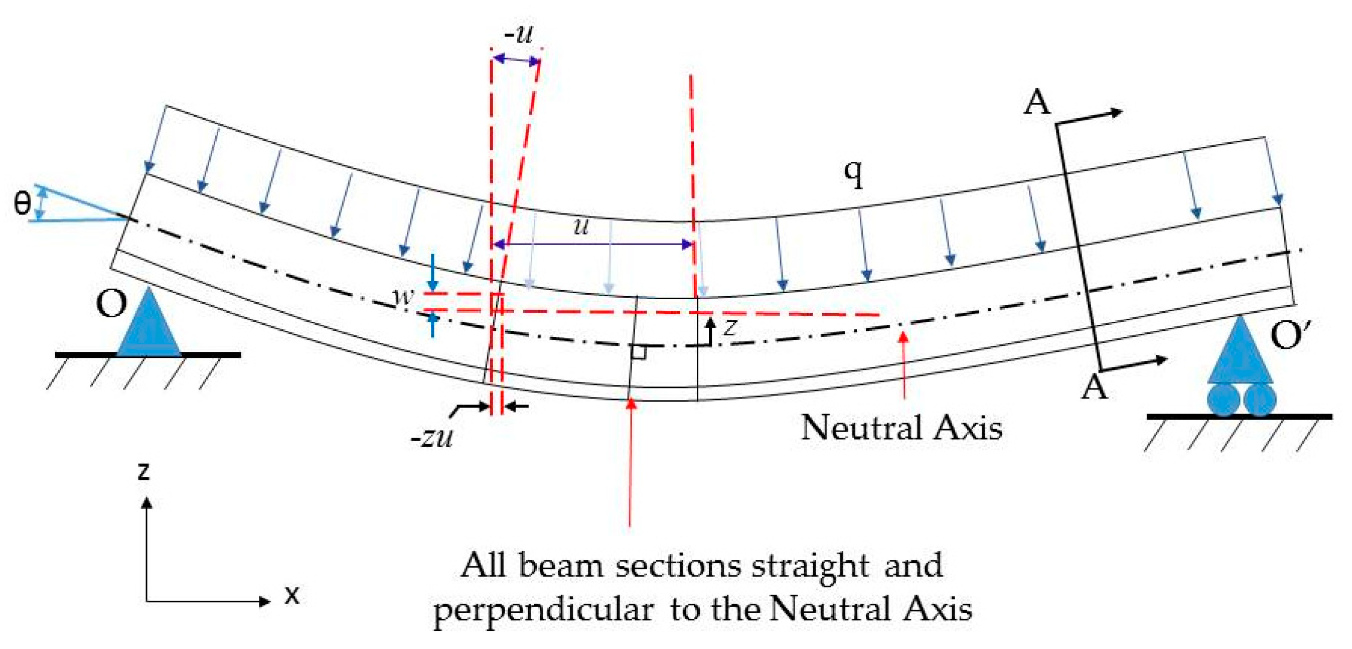
As shown in Figure 1, the assumptions made to calculate the displacement of the T-beam are as follows:

$$U\left(x,z\right)\approx u\left(x\right)-z{u}_1\left(x\right)$$

(1)

$$W\left(x,z\right)\approx w\left(x\right)$$

(2)

where U and W are the displacements of the beam after deformation.

The plane and shear strains are expressed as:

$${\epsilon }_x=\frac{\partial U}{\partial x}=u^{\prime }\left(x\right)-z{u}_1^{\prime }\left(x\right)$$

(3)

$${\gamma }_{xz}=\frac{\partial U}{\partial z}+\frac{\partial W}{\partial x}=-u_1\left(x\right)+w^{\prime }\left(x\right)$$

(4)

According to the Kirchhoff-Love hypothesis, the T-section perpendicular to the central axis of the beam remains perpendicular to the central axis after bending. Therefore, the shear strain ${\gamma }_{xz}$ is considered negligible in Equation (4). Hence,

$${\gamma }_{xz}=-u_1\left(x\right)+w^{\prime }\left(x\right)=0$$

(5)

$$\mathrm{then} u_1^{}\left(x\right)=w^{\prime }\left(x\right)$$

(6)

The strain is derived from Equations (3) and (6), as shown in Equation (7).

$$\epsilon x=u^{\prime }\left(x\right)-z{w}^{″}\left(x\right)$$

(7)

2.2. 2D Flange Normal Stress

The stress and strain on the neutral axis are zero; therefore, Equation (7) becomes

$$\epsilon x=-z{w}^{″}\left(x\right)$$

(8)

According to Hooke’s law [1] and the assumptions of beam theory, a 1D composite beam is subjected to a single axial strain ${\epsilon }_x$, that is, ${\epsilon }_y={\gamma }_{xy}=0$. The stress-strain relationship is expressed by Equation (9).

$${\sigma }_x={\overline{Q}}_{11}{\epsilon }_x$$

(9)

where ${\sigma }_x$ and ${\overline{Q}}_{11}$ are the normal stress of the flange and stiffness matrix, respectively.

By combining Equations (8) and (9), the ${\sigma }_x$ can be expressed as:

$${\sigma }_x={\overline{Q}}_{11}{\epsilon }_x={\overline{Q}}_{11}\left[-z{w}^{″}\left(x\right)\right]$$

(10)

As shown in Figure 1, the necessary condition for the beam to be in equilibrium is that the resultant normal force generated by ${\sigma }_x$ should be zero. Therefore, Equation (10) can be expanded as,

$${\displaystyle \sum _{k=1}^{N_w}{\overline{Q}}_{11,w}^k{\displaystyle {\int }_{A_f^k}\left[-z{w}^{″}\left(x\right)\right]}}dA+{\displaystyle \sum _{k=1}^{N_f}{\overline{Q}}_{11,f}^k{\displaystyle {\int }_{A_f^k}\left[-z{w}^{″}\left(x\right)\right]}}dA=0$$

(11)

$$({\displaystyle \sum _{k=1}^{N_w}{\overline{Q}}_{11,w}^k{\displaystyle {\int }_{A_w^k}\left[-z\right]}}dA+{\displaystyle \sum _{k=1}^{N_f}{\overline{Q}}_{11,f}^k{\displaystyle {\int }_{A_f^k}\left[-z\right]}}dA)w^{″}\left(x\right)=0$$

(12)

$${\displaystyle \sum _{k=1}^{N_w}{\overline{Q}}_{11,w}^k{\displaystyle {\int }_{A_w^k}\left[-z\right]}}dA+{\displaystyle \sum _{k=1}^{N_f}{\overline{Q}}_{11,f}^k{\displaystyle {\int }_{A_f^k}\left[-z\right]}}dA=0$$

(13)

Considering the bottom of the T-beam section as the reference plane, the distance of any lamination on the section from the centroid position is expressed as Equation (14).

$$z=Z^{\prime }-\overline{Z}$$

(14)

$${\displaystyle \sum _{k=1}^{N_w}{\overline{Q}}_{11,w}^k{\displaystyle {\int }_{A_w^k}\left[\overline{Z}-Z^{\prime }\right]}}dA+{\displaystyle \sum _{k=1}^{N_f}{\overline{Q}}_{11,f}^k{\displaystyle {\int }_{A_f^k}\left[\overline{Z}-Z^{\prime }\right]}}dA=0$$

(15)

$$\mathrm{where} {\displaystyle \int Z^{\prime }dA={\overline{Z}}_i}{A}_i$$

(16)

$$\mathrm{and} {\displaystyle \int \overline{Z}}dA=\overline{Z}{A}_i$$

(17)

$$\mathrm{Then} {\overline{Q}}_{11,w}^k{\displaystyle \sum _{k=1}^N}\left(\overline{Z}{A}_w-{\overline{Z}}_w{A}_w\right)+{\overline{Q}}_{11,f}^k{\displaystyle \sum _{k=1}^N}\left(\overline{Z}{A}_f-{\overline{Z}}_f{A}_f\right)=0$$

(18)

where ${\overline{Z}}_f$ and ${\overline{Z}}_w$ are the distances of each flange and web laminations, respectively, from the bottom of the section to the centroid. From Equation (18), the lateral centroid position is given as:

$$\overline{Z}=\frac{{\displaystyle \sum _{k=1}^N{\overline{Q}}_{11,f}^k{\overline{Z}}_f{A}_f+{\displaystyle \sum _{k=1}^N{\overline{Q}}_{11,w}^k{\overline{Z}}_w^{}{A}_w}}}{{\displaystyle \sum _{k=1}^N{\overline{Q}}_{11,f}^k{A}_f+{\displaystyle \sum _{k=1}^N{\overline{Q}}_{11,w}^k{A}_w}}}$$

(19)

The relationship between the resultant moment and stress is expressed as:

$$M_y={\displaystyle \sum _{k=1}^{Nw}{\overline{Q}}_{11,w}^k{\displaystyle {\int }_{A_w^k}\left[-z^2{w}^{″}\right]}}dA+{\displaystyle \sum _{k=1}^{N_f}{\overline{Q}}_{11,f}^k{\displaystyle {\int }_{A_f^k}\left[-z^2{w}^{″}\right]}}dA$$

(20)

$$\mathrm{Then} M_y=-\left[{\displaystyle \sum _{k=1}^{N_W}{\overline{Q}}_{11,w}^k{\displaystyle {\int }_{A_w^k}{z}^2}}dA+{\displaystyle \sum _{k=1}^{N_f}{\overline{Q}}_{11,f}^k{\displaystyle {\int }_{A_f^k}{z}^{2}dA}}\right]w^{″}\left(x\right)$$

(21)

The effective stiffness ($E{I}_{eff}$) of the laminated T-beam is defined as:

$$E{I}_{eff}=\left[{\displaystyle \sum _{k=1}^{N_w}{\overline{Q}}_{11,w}^k}{\displaystyle {\int }_{A_w^k}{z}^{2}dA}+{\displaystyle \sum _{k=1}^{N_f}{\overline{Q}}_{11,f}^k}{\displaystyle {\int }_{A_f^k}{z}^2}dA\right]$$

(22)

Therefore, the bending moment of the laminated T-beam is expressed as:

$$M_y=-\left(E{I}_{eff}\right)w^{″}\left(x\right)$$

(23)

The normal strain can be deduced from Equation (8) and Equation (23).

$${\epsilon }_x=\frac{z{M}_y}{E{I}_{eff}}$$

(24)

Therefore, the normal stress of the k^th layer of the flange is calculated using the relationship between stress and strain as shown in Equation (25):

$${\sigma }_x^k={\overline{Q}}_{11}^k\left(\frac{z{M}_y}{E{I}_{eff}}\right)$$

(25)

2.3. Centroid Position in 2D Theoretical Analysis

A laminated T-beam was divided into two laminated plates: the web and the flange. The formulas for the web and flange were derived based on the beam theory and composite laminated ABD matrix, respectively. The basic assumptions used in the 2D composite beam theory are as follows: (1) The deflection of the beam is smaller than the length of the beam. Consequently, the slope of the deflection curve is small, and the square of the slope is significantly lesser than one. Therefore, it can be ignored. (2) The section originally perpendicular to the central axis of the beam remains flat after bending and is perpendicular to the central axis after bending.

In the analysis process, the flanges of the T-beams were divided into narrow and wide flanges. In a narrow flange, the beam width was assumed to be approximately equal to the beam height. Geometrically, this type of flange can be regarded as a beam structure. When the beam structure is subjected to a lateral load, strain occurs laterally. Therefore, the moment generated laterally can be disregarded. In a wide flange, the beam width was assumed to be significantly higher than the beam height. Geometrically, this type of flange can be considered as a thin plate where a lateral moment exists because the thin-plate structure cannot deform laterally after it is subjected to a lateral load. As the carbon fiber-composite laminate beams were combined layer-by-layer by arranging in different directions, resulting in a difference between symmetric and non-symmetric fibers according to the fiber direction. Stress analysis for symmetric and non-symmetric structures was included in the analytical solution.

2.3.1. Symmetrical Laminated Composite T-Beam Center Position

• Narrow flange center position

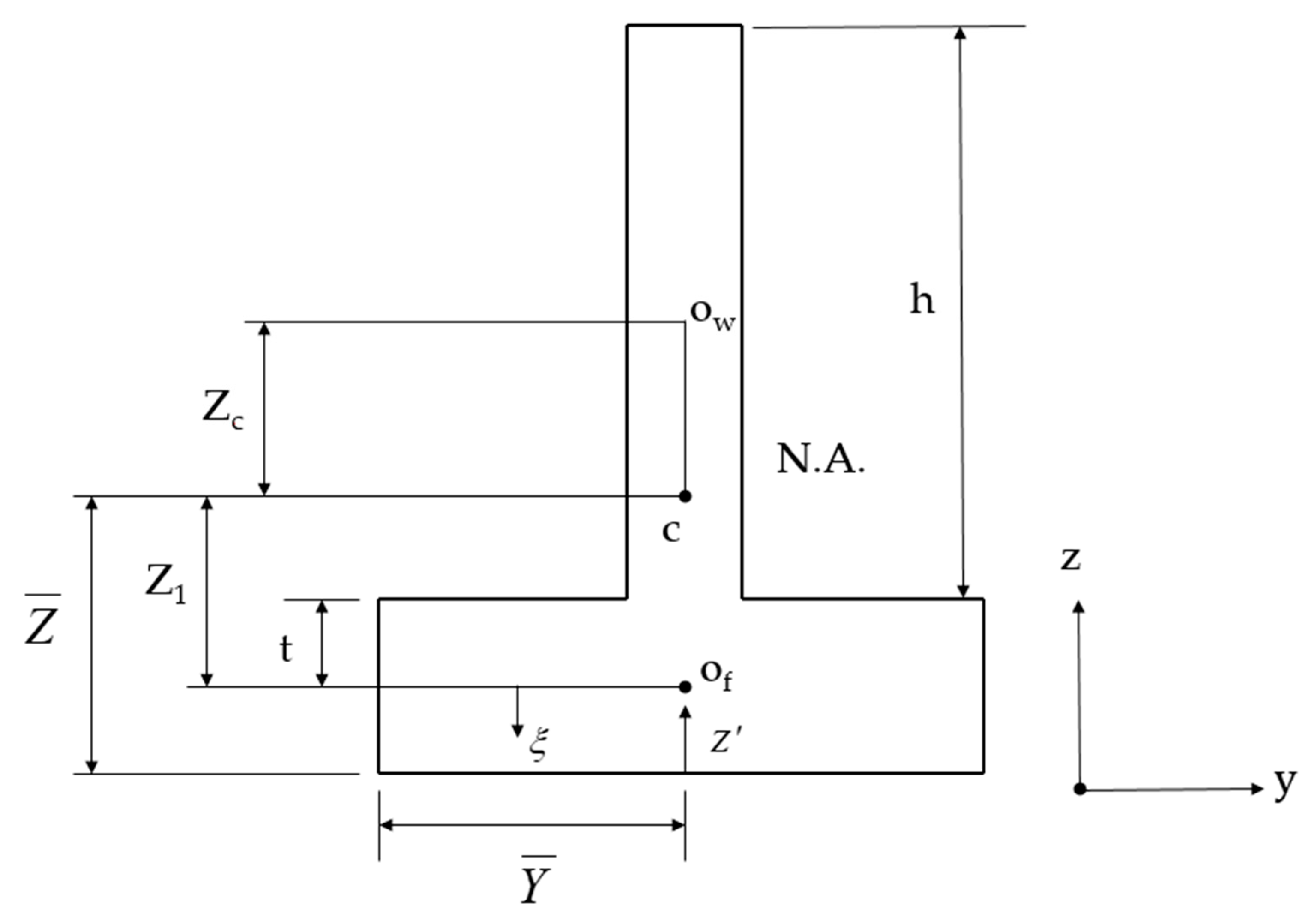
As shown in Figure 2, under the lateral load, the resultant lateral force $N_y=0$ and the bending moment $M_y=0$. The relationship between the strain and resultant force and the curvature and resultant moment of the narrow-flange laminated T-beam are as follows:

$$\left\{\begin{array}{c}{\epsilon }_x^0\\ {\epsilon }_y^0\\ {\epsilon }_{xy}^0\end{array}\right\}=\left[A^{-1}\right]\left\{\begin{array}{c}{N}_x\\ 0\\ 0\end{array}\right\}, \left\{\begin{array}{c}{\kappa }_x\\ {\kappa }_y\\ {\kappa }_{xy}\end{array}\right\}=\left[D^{-1}\right]\left\{\begin{array}{c}{M}_x\\ 0\\ 0\end{array}\right\}$$

(26)

By simplifying Equation (26) to Equation (27):

$$N_x=\frac{1}{A_{11}^{-1}}{\epsilon }_x^0=\frac{Z_1}{A_{11}^{-1}}{\kappa }_x \mathrm{and} M_x=\frac{1}{D_{11}^{-1}}{\kappa }_x$$

(27)

The stress of the T-beam is zero at the neutral axis, as shown in Figure 1. Therefore, the sum of the stresses of the web and flange is zero Equation (28).

$$N_{x,w}+N_{x,f}=0$$

(28)

The resultant stresses of the web and flange are derived from Equation (27), and shown in Equations (29) and (30):

$$N_{x,w}={\displaystyle {\int }_{-\frac{h}{2}+Z_c}^{\frac{h}{2}+Z_c}{N}_x}dz={\displaystyle {\int }_{-\frac{h}{2}+Z_c}^{\frac{h}{2}+Z_c}\frac{z}{A_{11,w}^{-1}}{\kappa }_{x}dz=\frac{h{Z}_c}{A_{11,w}^{-1}}}{\kappa }_x$$

(29)

$$N_{x,f}=b{N}_x=b\left(\frac{1}{A_{11,f}^{-1}}{\epsilon }_x^0\right)=b\left(\frac{Z_1}{A_{11,f}^{-1}}\right){\kappa }_x=b\left(\frac{-\frac{h}{2}+Z_c-t}{A_{11,f}^{-1}}\right){\kappa }_x$$

(30)

$$\mathrm{where} Z_1=\left|\frac{-h}{2}+Z_c-t\right|$$

(31)

By substituting Equations (29) and (30) into Equation (28):

$$\left(\frac{h{Z}_c}{A_{11,w}^{-1}}+\frac{b\left(-\frac{h}{2}+Z_c-t\right)}{A_{11,f}^{-1}}\right){\kappa }_x=0$$

(32)

where $t$ is the distance from the flange centroid, $o_f$ to the outermost layer of the flange, $Z_1$ is the distance from the centroid $c$ to $o_f$, $Z_c$ is the distance from $c$ to the centroid of the web. The $o_w$ can be calculated for the laminated narrow flange composite T-beam shown in Equation (33).

$$Z_c=\frac{\frac{h}{2}+t}{1+\frac{h{A}_{11,f}^{-1}}{b{A}_{11,w}^{-1}}}$$

(33)

• Wide flange center position

Under the assumption of a wide symmetrical flange, $\left[B\right]=0$. Transverse resultant force $N_y=0$, $N_{xy}=0$, and transverse curvature ${\kappa }_y=0$, ${\kappa }_{xy}=0$. The relationship between the strain and resultant force and the curvature and resultant moment of the wide-flange laminated T-beam becomes:

$$\left\{\begin{array}{c}{N}_x\\ 0\\ 0\\ M_x\\ M_y\\ M_{xy}\end{array}\right\}=\left[\begin{array}{cccccc}{A}_{11}& A_{12}& A_{13}& 0& 0& 0\\ A_{21}& A_{22}& A_{23}& 0& 0& 0\\ A_{31}& A_{32}& A_{33}& 0& 0& 0\\ 0& 0& 0& D_{11}& D_{12}& D_{13}\\ 0& 0& 0& D_{21}& D_{22}& D_{23}\\ 0& 0& 0& D_{31}& D_{32}& D_{33}\end{array}\right]\left\{\begin{array}{c}{\epsilon }_x^0\\ {\epsilon }_y^0\\ {\gamma }_{xy}^0\\ {\kappa }_x\\ 0\\ 0\end{array}\right\}$$

(34)

where A and D are laminate-stiffness matrices. Equation (34) can be simplified as follows:

$$N_x=\frac{1}{A_{11}^{-1}}{\epsilon }_x^0=\frac{Z_1}{A_{11}^{-1}}{\kappa }_x \mathrm{and} M_x=\frac{1}{D_{11}^{-1}}{\kappa }_x$$

(35)

The stress of the T-beam is zero at the neutral axis, as shown in Figure 1. Therefore, the sum of the stresses in the web and flange is zero Equation (36).

$$N_{x,w}+N_{x,f}=0$$

(36)

The resultant stresses of the web and flange are derived from Equation (35) and are shown in Equations (37) and (38).

$$N_{x,w}={\displaystyle {\int }_{-\frac{h}{2}+Z_c}^{\frac{h}{2}+Z_c}{N}_x}dz={\displaystyle {\int }_{-\frac{h}{2}+Z_c}^{\frac{h}{2}+Z_c}\frac{z}{A_{11,w}^{-1}}{\kappa }_{x}dz=\frac{h{Z}_c}{A_{11,w}^{-1}}}{\kappa }_x$$

(37)

$$N_{x,f}=b{N}_x=b\left(\frac{1}{A_{11,f}^{-1}}{\epsilon }_x^0\right)=b\left(\frac{Z_1}{A_{11,f}^{-1}}\right){\kappa }_x=b\left(\frac{-\frac{h}{2}+Z_c-t}{A_{11,f}^{-1}}\right){\kappa }_x$$

(38)

$$\mathrm{where} Z_1=\left|\frac{-h}{2}+Z_c-t\right|$$

(39)

Equations (37) and (38) are substituted into Equation (36) to obtain Equation (40).

$$\left(\frac{h{Z}_c}{A_{11,w}^{-1}}+\frac{b\left(-\frac{h}{2}+Z_c-t\right)}{A_{11,f}^{-1}}\right){\kappa }_x=0$$

(40)

The $o_w$ can be obtained for the laminated wide-flange composite T-beam shown in Equation (41).

$$Z_c=\frac{\frac{h}{2}+t}{1+\frac{h{A}_{11,f}^{-1}}{b{A}_{11,w}^{-1}}}$$

(41)

2.3.2. Centroid Position of Nonsymmetrical Laminated Composite T-Beams

• Narrow flange centroid position

The [B] matrices are part of the non-symmetric matrices; therefore, the F matrix is used to represent the inverse of the ABD matrix, as shown in Equation (42):

$$\left[F\right]\equiv {\left[\begin{array}{cc}A& B\\ B& D\end{array}\right]}^{-1}$$

(42)

Using the assumption of a narrow beam: $M_y=M_{xy}=0$; therefore, only the axial resultant force N_x and the resultant bending moment M_x exist. The relationships between the strain and resultant force and the curvature and resultant moment of the nonsymmetric narrow flange T-beam are expressed as follows:

$$\left\{\begin{array}{c}{\epsilon }_x^0\\ {\epsilon }_y^0\\ {\gamma }_{xy}^0\\ {\kappa }_x\\ {\kappa }_y\\ {\kappa }_{xy}\end{array}\right\}=\left[\begin{array}{cccccc}{F}_{11}& F_{12}& F_{12}& F_{14}& F_{15}& F_{16}\\ F_{21}& F_{22}& F_{23}& F_{24}& F_{25}& F_{26}\\ F_{31}& F_{32}& F_{33}& F_{34}& F_{35}& F_{36}\\ F_{41}& F_{42}& F_{43}& F_{44}& F_{45}& F_{46}\\ F_{51}& F_{52}& F_{53}& F_{54}& F_{55}& F_{56}\\ F_{61}& F_{62}& F_{63}& F_{64}& F_{65}& F_{66}\end{array}\right]\left\{\begin{array}{c}{N}_x\\ 0\\ 0\\ M_x\\ 0\\ 0\end{array}\right\}$$

(43)

By expanding and simplifying Equation (43), $N_x$ and $M_x$ are deduced as follows:

$$\begin{gathered} N_x=\frac{F_{44}}{\mathsf{\Delta }}{\epsilon }_x^0-\frac{F_{14}}{\mathsf{\Delta }}{\kappa }_x, M_x=\frac{-F_{41}}{\mathsf{\Delta }}{\epsilon }_x^0+\frac{F_{11}}{\mathsf{\Delta }}{\kappa }_x \\ \mathsf{\Delta }\equiv F_{11}{F}_{44}-F_{14}{F}_{41} \end{gathered}$$

(44)

The resultant stresses of the web and flange are derived from Equation (44), as shown in Equation (45) and Equation (46), respectively,

$$N_{x,w}={\displaystyle {\int }_{-\frac{h}{2}+Z_c}^{\frac{h}{2}+Z_c}{N}_x}dz={\displaystyle {\int }_{-\frac{h}{2}+Z_c}^{\frac{h}{2}+Z_c}\frac{z}{A_{11,w}^{-1}}{\kappa }_{x}dz=\frac{h{Z}_c}{A_{11,w}^{-1}}}{\kappa }_x$$

(45)

$$N_{x,f}=b{N}_x=b\left(\frac{F_{44}}{\mathsf{\Delta }}{Z}_1{\kappa }_x-\frac{F_{14}}{\mathsf{\Delta }}{\kappa }_x\right)=b\left[\left(\frac{F_{44}}{\mathsf{\Delta }}\left(\frac{-h}{2}+Z_c-t\right)-\frac{F_{14}}{\mathsf{\Delta }}\right)\right]{\kappa }_x$$

(46)

The stress of the T-beam is zero at the neutral axis, as shown in Figure 1. Therefore, the sum of the stresses in the web and flange is zero, as shown in Equation (47).

$$N_{x,w}+N_{x,f}=0$$

(47)

Equations (45) and (46) are substituted into Equation (47):

$$\left[\frac{h{Z}_c}{A_{11,w}^{-1}}+\frac{b{F}_{44}}{\mathsf{\Delta }}\left(\frac{-h}{2}+Z_c-t\right)-\frac{b{F}_{14}}{\mathsf{\Delta }}\right]{\kappa }_x=0$$

(48)

The $o_w$ can be obtained for the laminated narrow-flange composite T beam shown in Equation (49).

$$Z_c=\frac{\frac{b}{\mathsf{\Delta }}\left(\frac{h{F}_{44}}{2}+t{F}_{44}+F_{14}\right)}{\left(\frac{h}{A_{11,w}^{-1}}+\frac{b{F}_{44}}{\mathsf{\Delta }}\right)}$$

(49)

• Wide flange centroid position

Using the assumption of ${\kappa }_y={\kappa }_{xy}=0$ for a wide beam, the relationships between the strain and resultant force and the curvature and resultant moment of the nonsymmetric wide flange T-beam are as follows:

$$\left\{\begin{array}{c}{N}_x\\ 0\\ 0\\ M_x\\ M_y\\ M_{xy}\end{array}\right\}=\left[\begin{array}{cccccc}{A}_{11}& A_{12}& A_{13}& B_{11}& B_{12}& B_{13}\\ A_{21}& A_{22}& A_{23}& B_{21}& B_{22}& B_{23}\\ A_{31}& A_{32}& A_{33}& B_{31}& B_{32}& B_{33}\\ B_{11}& B_{12}& B_{13}& D_{11}& D_{12}& D_{13}\\ B_{21}& B_{22}& B_{23}& D_{21}& D_{22}& D_{23}\\ B_{31}& B_{32}& B_{33}& D_{31}& D_{32}& D_{33}\end{array}\right]\left\{\begin{array}{c}{\epsilon }_x^0\\ {\epsilon }_y^0\\ {\gamma }_{xy}^0\\ {\kappa }_x\\ 0\\ 0\end{array}\right\}$$

(50)

The inverse matrix of the ABD matrix Equation (50), represented by the F matrix, becomes Equation (51):

$$\left\{\begin{array}{c}{\epsilon }_x^0\\ {\epsilon }_y^0\\ {\gamma }_{xy}^0\\ {\kappa }_x\\ 0\\ 0\end{array}\right\}=\left[\begin{array}{cccccc}{F}_{11}& F_{12}& F_{12}& F_{14}& F_{15}& F_{16}\\ F_{21}& F_{22}& F_{23}& F_{24}& F_{25}& F_{26}\\ F_{31}& F_{32}& F_{33}& F_{34}& F_{35}& F_{36}\\ F_{41}& F_{42}& F_{43}& F_{44}& F_{45}& F_{46}\\ F_{51}& F_{52}& F_{53}& F_{54}& F_{55}& F_{56}\\ F_{61}& F_{62}& F_{63}& F_{64}& F_{65}& F_{66}\end{array}\right]\left\{\begin{array}{c}{N}_x\\ 0\\ 0\\ M_x\\ M_y\\ M_{xy}\end{array}\right\}$$

(51)

Equation (51) is simplified to Equation (52). The new simplified matrix is called a G matrix.

$$\left\{\begin{array}{c}{\epsilon }_x^0\\ {\kappa }_x^{}\\ 0\\ 0\end{array}\right\}=\left[\begin{array}{cccc}{F}_{11}& F_{14}& F_{15}& F_{16}\\ F_{41}& F_{44}& F_{45}& F_{46}\\ F_{51}& F_{54}& F_{55}& F_{56}\\ F_{61}& F_{64}& F_{65}& F_{66}\end{array}\right]\left\{\begin{array}{c}{N}_x\\ M_x\\ M_y\\ M_{xy}\end{array}\right\}=\left[\begin{array}{cccc}{G}_{11}& G_{12}& G_{13}& G_{14}\\ G_{21}& G_{22}& G_{23}& G_{24}\\ G_{31}& G_{32}& G_{33}& G_{34}\\ G_{41}& G_{42}& G_{43}& G_{44}\end{array}\right]\left\{\begin{array}{c}{N}_x\\ M_x\\ M_y\\ M_{xy}\end{array}\right\}$$

(52)

$$\left\{\begin{array}{c}{N}_x\\ M_x\\ M_y\\ M_{xy}\end{array}\right\}={\left[\begin{array}{cccc}{G}_{11}& G_{12}& G_{13}& G_{14}\\ G_{21}& G_{22}& G_{23}& G_{24}\\ G_{31}& G_{32}& G_{33}& G_{34}\\ G_{41}& G_{42}& G_{43}& G_{44}\end{array}\right]}^{-1}\left\{\begin{array}{c}{\epsilon }_x^0\\ {\kappa }_x^{}\\ 0\\ 0\end{array}\right\}$$

(53)

From Equation (53), the axial stress of the flange is:

$$N_x=G_{11}^{-1}{\epsilon }_x^0+G_{12}^{-1}{\kappa }_x=\left(Z_1{G}_{11}^{-1}+G_{12}^{-1}\right){\kappa }_x$$

(54)

The resultant stress of the web and flange is derived using Equation (54) as follows:

$$N_{x,w}={\displaystyle {\int }_{-\frac{h}{2}+Z_c}^{\frac{h}{2}+Z_c}{N}_x}dz={\displaystyle {\int }_{-\frac{h}{2}+Z_c}^{\frac{h}{2}+Z_c}\frac{z}{A_{11,w}^{-1}}{\kappa }_{x}dz=\frac{h{Z}_c}{A_{11,w}^{-1}}}{\kappa }_x$$

(55)

$$N_{x,f}=b{N}_x=b\left(G_{11}^{-1}{Z}_1{\kappa }_x+G_{12}^{-1}{\kappa }_x\right)=b\left[G_{11}^{-1}\left(\frac{-h}{2}+Z_c-t\right)+G_{12}^{-1}\right]{\kappa }_x$$

(56)

As shown in Figure 1, the stress of the T-beam was zero at the neutral axis. Therefore, the sum of the stresses in the web and flange was zero, as shown in Equation (57).

$$N_{x,w}+N_{x,f}=0$$

(57)

Substitute Equations (55) and (56) into Equation (57) to obtain Equation (58)

$$\left(\frac{h{Z}_c}{A_{11,w}^{-1}}-\frac{b{G}_{11}^{-1}h}{2}+b{G}_{11}^{-1}{Z}_c-b{G}_{11}^{-1}t+b{G}_{12}^{-1}\right){\kappa }_x=0$$

(58)

The $o_w$ can be obtained for the laminated wide-flange composite T-beam, as shown in Equation (59).

$$Z_c=\frac{\frac{b{G}_{11}^{-1}h}{2}+b{G}_{11}^{-1}t-b{G}_{12}^{-1}}{\frac{h}{A_{11,w}^{-1}}+b{G}_{11}^{-1}}$$

(59)

2.4. Stress and Strain of Symmetrical Laminated Composite T-Beams

The T-shaped composite beam was divided into two parts for analysis: the web and the flange. The effective stiffness ($E{I}_{eff}$) of the beam was calculated from the sum of the moments of the web and flange.

2.4.1. Narrow Flange

The sum of the stresses and moments on the web is given as shown in Equations (60) and (61).

$$N_{x,w}=\left(\frac{1}{A_{11,w}^{-1}}\right)z{\kappa }_x$$

(60)

$$M_{web}={\displaystyle {\int }_{-\frac{h}{2}+Z_c}^{\frac{h}{2}+Z_c}{N}_{x,w}zdz}={\displaystyle {\int }_{-\frac{h}{2}+Z_c}^{\frac{h}{2}+Z_c}\frac{z^2}{A_{11,w}^{-1}}}{\kappa }_{x}dz=\frac{{\kappa }_x}{A_{11,w}^{-1}}\left(\frac{h^3}{12}+h{Z}_c^2\right)$$

(61)

The moment of the narrow flange is calculated using Equation (26):

$$M_{flange}=b\left(N_x{Z}_1+M_x\right)=b\left(\frac{Z_1^2}{A_{11,f}^{-1}}+\frac{1}{D_{11,f}^{-1}}\right){\kappa }_x$$

(62)

The moment of the beam is the sum of the moments of the flange and web, which is derived using Equations (61) and (62):

$$M_{beam}=M_{web}+M_{flange}=\left[\left(\frac{h^3}{12A_{11,w}^{-1}}+\frac{Z_c^{2}h}{A_{11,w}^{-1}}\right)+b\left(\frac{Z_1^2}{A_{11,f}^{-1}}+\frac{1}{D_{11,f}^{-1}}\right)\right]{\kappa }_x=E{I}_{eff}{\kappa }_x$$

(63)

From Equation (63) the effective stiffness of the beam is given as:

$$E{I}_{eff}=\left(\frac{h^3}{12A_{11,w}^{-1}}+\frac{Z_c^{2}h}{A_{11,w}^{-1}}\right)+b\left(\frac{Z_1^2}{A_{11,f}^{-1}}+\frac{1}{D_{11,f}^{-1}}\right)$$

(64)

The strain of the beam in the x-axis direction is expressed as shown in Equation (65)

$${\epsilon }_x=z{\kappa }_x$$

(65)

The strains of the flange in the x- and y-axis directions are given as:

$${\epsilon }_x={\epsilon }_x^0+\xi {\kappa }_x=\left(Z_1+\xi \right){\kappa }_x, {\epsilon }_y={\epsilon }_y^0+\xi {\kappa }_y=\left[\frac{A_{21,f}^{-1}}{A_{11,f}^{-1}}{Z}_1+\xi \frac{D_{21,f}^{-1}}{D_{11,f}^{-1}}\right]{\kappa }_x$$

(66)

The shear strain of the flange in the xy plane is:

$${\gamma }_{xy}=(Z_1\frac{A_{31,f}^{-1}}{A_{11,f}^{-1}}+\xi \frac{D_{31,f}^{-1}}{D_{11,f}^{-1}}){\kappa }_x$$

(67)

Therefore, the total strain of the narrow flange is given as:

$$\left\{\begin{array}{c}{\epsilon }_x\\ {\epsilon }_y\\ {\gamma }_{xy}\end{array}\right\}=\left\{\begin{array}{c}{Z}_1+\xi \\ Z_1\frac{A_{21,f}^{-1}}{A_{11,f}^{-1}}+\xi \frac{D_{21,f}^{-1}}{D_{11,f}^{-1}}\\ Z_1\frac{A_{31,f}^{-1}}{A_{11,f}^{-1}}+\xi \frac{D_{31,f}^{-1}}{D_{11,f}^{-1}}\end{array}\right\}{\kappa }_x$$

(68)

The stress on the beam is derived from the stress-strain relation, as shown in Equation (69):

$$\left\{\begin{array}{c}{\sigma }_x^{}\\ {\sigma }_y^{}\\ {\tau }_{xy}^{}\end{array}\right\}=\left[\begin{array}{ccc}{\overline{Q}}_{11}& {\overline{Q}}_{12}& {\overline{Q}}_{16}\\ {\overline{Q}}_{21}& {\overline{Q}}_{22}& {\overline{Q}}_{26}\\ {\overline{Q}}_{61}& {\overline{Q}}_{62}& {\overline{Q}}_{66}\end{array}\right]\left\{\begin{array}{c}{\epsilon }_x^{}\\ {\epsilon }_y^{}\\ {\gamma }_{xy}^{}\end{array}\right\}$$

(69)

2.4.2. Wide Flange

The sum of moments on the web is calculated as shown in Equation (61). The moment of the flange is derived using Equation (35) and shown in Equation (70).

$$M_{flange}=b\left(N_x{Z}_1+M_x\right)=b\left(\frac{Z_1^2}{A_{11,f}^{-1}}+D_{11,f}\right){\kappa }_x$$

(70)

From Equations (61) and (70), the sum of the T-beam moments can be obtained.

$$M_{beam}=M_{web}+M_{flange}=\left[\left(\frac{h^3}{12A_{11,w}^{-1}}+\frac{Z_c^{2}h}{A_{11,w}^{-1}}\right)+b\left(\frac{Z_1^2}{A_{11,f}^{-1}}+D_{11,f}\right)\right]{\kappa }_x=E{I}_{eff}{\kappa }_x$$

(71)

The effective stiffness of the beam can be obtained as well.

$$E{I}_{eff}=\left(\frac{h^3}{12A_{11,w}^{-1}}+\frac{Z_c^{2}h}{A_{11,w}^{-1}}\right)+b\left(\frac{Z_1^2}{A_{11,f}^{-1}}+D_{11,f}\right)$$

(72)

The strain of the flange is as follows

$$\left\{\begin{array}{c}{\epsilon }_x\\ {\epsilon }_y\\ {\gamma }_{xy}\end{array}\right\}=\left\{\begin{array}{c}{Z}_1+\xi \\ Z_1\frac{A_{21,f}^{-1}}{A_{11,f}^{-1}}\\ Z_1\frac{A_{31,f}^{-1}}{A_{11,f}^{-1}}\end{array}\right\}{\kappa }_x$$

(73)

The stress for each laminate can be calculated using Equation (69).

2.5. Stress and Strain of Nonsymmetric Laminated Composite T-Beam

2.5.1. Narrow Flange

The sum of the moments on the web is given in Equation (61).

The sum of the flange moment is derived from Equation (44) and is expressed as:

$$M_{flange}=b\left(N_x{Z}_1+M_x\right)=b\left[\left(\frac{F_{44}}{\mathsf{\Delta }}{Z}_1^2-\frac{F_{14}}{\mathsf{\Delta }}{Z}_1\right)+\left(\frac{-F_{41}}{\mathsf{\Delta }}{Z}_1+\frac{F_{11}}{\mathsf{\Delta }}\right)\right]{\kappa }_x$$

(74)

Therefore, the moment of the beam is calculated by combining Equations (61) and (74).

$$M_{beam}=M_{web}+M_{flange}=\left[\left(\frac{h^3}{12A_{11,w}^{-1}}+\frac{Z_c^{2}h}{A_{11,w}^{-1}}\right)+b\left(\begin{array}{l}\left(\frac{F_{44}}{\mathsf{\Delta }}{Z}_1^2-\frac{F_{14}}{\mathsf{\Delta }}{Z}_1\right)\\ +\left(\frac{-F_{41}}{\mathsf{\Delta }}{Z}_1+\frac{F_{11}}{\mathsf{\Delta }}\right)\end{array}\right)\right]{\kappa }_x=E{I}_{eff}{\kappa }_x$$

(75)

Consequently, the effective stiffness of the narrow flange is expressed as:

$$E{I}_{eff}=\left(\frac{h^3}{12A_{11,w}^{-1}}+\frac{Z_c^{2}h}{A_{11,w}^{-1}}\right)+b\left[\left(\frac{F_{44}{Z}_1}{\mathsf{\Delta }}-\frac{F_{14}}{\mathsf{\Delta }}\right)Z_1+\left(\frac{-F_{41}{Z}_1}{\mathsf{\Delta }}+\frac{F_{11}}{\mathsf{\Delta }}\right)\right]$$

(76)

The strain of the beam in the x-axis direction is given by Equation (65).

The strain of the flange is expressed as Equation (77) by combining Equations (12) and (43).

$$\left\{\begin{array}{c}{\epsilon }_x\\ {\epsilon }_y\\ {\gamma }_{xy}\end{array}\right\}=\left\{\begin{array}{c}{F}_{11}{N}_x+F_{14}{M}_x\\ F_{21}{N}_x+F_{24}{M}_x\\ F_{31}{N}_x+F_{34}{M}_x\end{array}\right\}+\xi \left\{\begin{array}{c}{\kappa }_x\\ {\kappa }_y\\ {\kappa }_{xy}\end{array}\right\}$$

(77)

$$\mathrm{Then} \left\{\begin{array}{c}{\epsilon }_x\\ {\epsilon }_y\\ {\gamma }_{xy}\end{array}\right\}=\left\{\begin{array}{c}{F}_{11}{N}_x+F_{14}{M}_x\\ F_{21}{N}_x+F_{24}{M}_x\\ F_{31}{N}_x+F_{34}{M}_x\end{array}\right\}+\xi \left\{\begin{array}{c}{\kappa }_x\\ F_{51}{N}_x+F_{54}{M}_x\\ F_{61}{N}_x+F_{64}{M}_x\end{array}\right\}$$

(78)

2.5.2. Wide Flange

The assumption used for the nonsymmetric wide flange was that the resultant transverse force $N_y=0$ and transverse curvature ${\kappa }_y$ = 0; therefore, the relationships between the strain and resultant force and the curvature and resultant moment of the T-beam are as follows:

$$\left\{\begin{array}{c}{N}_x\\ 0\\ 0\\ M_x\\ M_y\\ M_{xy}\end{array}\right\}=\left[\begin{array}{cccccc}{A}_{11}& A_{12}& A_{13}& B_{11}& B_{12}& B_{13}\\ A_{21}& A_{22}& A_{23}& B_{21}& B_{22}& B_{23}\\ A_{31}& A_{32}& A_{33}& B_{31}& B_{32}& B_{33}\\ B_{11}& B_{12}& B_{13}& D_{11}& D_{12}& D_{13}\\ B_{21}& B_{22}& B_{23}& D_{21}& D_{22}& D_{23}\\ B_{31}& B_{32}& B_{33}& D_{31}& D_{32}& D_{33}\end{array}\right]\left\{\begin{array}{c}{\epsilon }_x^0\\ {\epsilon }_y^0\\ {\gamma }_{xy}\\ {\kappa }_x\\ 0\\ 0\end{array}\right\}$$

(79)

The F matrix was used to represent the inverse of the ABD matrix; thus Equation (79) becomes:

$$\left\{\begin{array}{c}{\epsilon }_x^0\\ {\epsilon }_y^0\\ {\gamma }_{xy}^0\\ {\kappa }_x\\ 0\\ 0\end{array}\right\}=\left[\begin{array}{cccccc}{F}_{11}& F_{12}& F_{12}& F_{14}& F_{15}& F_{16}\\ F_{21}& F_{22}& F_{23}& F_{24}& F_{25}& F_{26}\\ F_{31}& F_{32}& F_{33}& F_{34}& F_{35}& F_{36}\\ F_{41}& F_{42}& F_{43}& F_{44}& F_{45}& F_{46}\\ F_{51}& F_{52}& F_{53}& F_{54}& F_{55}& F_{56}\\ F_{61}& F_{62}& F_{63}& F_{64}& F_{65}& F_{66}\end{array}\right]\left\{\begin{array}{c}{N}_x\\ 0\\ 0\\ M_x\\ M_y\\ M_{xy}\end{array}\right\}$$

(80)

Equation (80) is simplified to Equation (81). The new simplified matrix is called the G matrix.

$$\left\{\begin{array}{c}{\epsilon }_x^0\\ {\kappa }_x^{}\\ 0\\ 0\end{array}\right\}=\left[\begin{array}{cccc}{F}_{11}& F_{14}& F_{15}& F_{16}\\ F_{41}& F_{44}& F_{45}& F_{46}\\ F_{51}& F_{54}& F_{55}& F_{56}\\ F_{61}& F_{64}& F_{65}& F_{66}\end{array}\right]\left\{\begin{array}{c}{N}_x\\ M_x\\ M_y\\ M_{xy}\end{array}\right\}=\left[\begin{array}{cccc}{G}_{11}& G_{12}& G_{13}& G_{14}\\ G_{21}& G_{22}& G_{23}& G_{24}\\ G_{31}& G_{32}& G_{33}& G_{34}\\ G_{41}& G_{42}& G_{43}& G_{44}\end{array}\right]\left\{\begin{array}{c}{N}_x\\ M_x\\ M_y\\ M_{xy}\end{array}\right\}$$

(81)

$$\left\{\begin{array}{c}{N}_x\\ M_x\\ M_y\\ M_{xy}\end{array}\right\}={\left[\begin{array}{cccc}{G}_{11}& G_{12}& G_{13}& G_{14}\\ G_{21}& G_{22}& G_{23}& G_{24}\\ G_{31}& G_{32}& G_{33}& G_{34}\\ G_{41}& G_{42}& G_{43}& G_{44}\end{array}\right]}^{-1}\left\{\begin{array}{c}{\epsilon }_x^0\\ {\kappa }_x^{}\\ 0\\ 0\end{array}\right\}$$

(82)

Subsequently, the stress, moment, and curvature of the flange are expressed as Equations (83)–(86)

$$N_x=G_{11}^{-1}{\epsilon }_x^0+G_{12}^{-1}{\kappa }_x=\left(Z_1{G}_{11}^{-1}+G_{12}^{-1}\right) {\kappa }_x$$

(83)

$$M_x=G_{21}^{-1}{\epsilon }_x^0+G_{22}^{-1}{\kappa }_x=\left(Z_1{G}_{21}^{-1}+G_{22}^{-1}\right) {\kappa }_x$$

(84)

$$M_y=G_{31}^{-1}{\epsilon }_x^0+G_{32}^{-1}{\kappa }_x=\left(Z_1{G}_{31}^{-1}+G_{32}^{-1}\right) {\kappa }_x$$

(85)

$$M_{xy}=G_{41}^{-1}{\epsilon }_x^0+G_{42}^{-1}{\kappa }_x=\left(Z_1{G}_{41}^{-1}+G_{42}^{-1}\right) {\kappa }_x$$

(86)

The total moment of the flange is

$$M_{flange}=b\left(N_x{Z}_1+M_x\right)=b\left[\left(G_{11}^{-1}{Z}_1^2+G_{12}^{-1}{Z}_1\right)+\left(G_{21}^{-1}{Z}_1+G_{22}^{-1}\right)\right] {\kappa }_x$$

(87)

Consequently, the total moment of the beam can be expressed as:

$$M_{beam}=M_{web}+M_{flange}=\left[\left(\frac{h^3}{12A_{11,w}^{-1}}+\frac{Z_c^{2}h}{A_{11,w}^{-1}}\right)+b\left(\left(G_{11}^{-1}{Z}_1^2+G_{12}^{-1}{Z}_1\right)+\left(G_{21}^{-1}{Z}_1+G_{22}^{-1}\right)\right)\right]{\kappa }_x=E{I}_{eff}{\kappa }_x$$

(88)

The effective stiffness of the wide flange can be expressed as:

$$E{I}_{eff}=\left(\frac{h^3}{12A_{11,w}^{-1}}+\frac{Z_c^{2}h}{A_{11,w}^{-1}}\right)+b\left[G_{11}^{-1}{Z}_1^2+\left(G_{12}^{-1}+G_{21}^{-1}\right)Z_1+G_{22}^{-1}\right]$$

(89)

The strain of the flange at each laminate is:

$$\left\{\begin{array}{c}{\epsilon }_x\\ {\epsilon }_y\\ {\gamma }_{xy}\end{array}\right\}=\left\{\begin{array}{cccc}{F}_{11}& F_{14}& F_{15}& F_{16}\\ F_{21}& F_{24}& F_{25}& F_{26}\\ F_{31}& F_{34}& F_{35}& F_{36}\end{array}\right\}\left\{\begin{array}{c}{Z}_1{G}_{11}^{-1}+G_{12}^{-1}\\ Z_1{G}_{21}^{-1}+G_{22}^{-1}\\ Z_1{G}_{31}^{-1}+G_{32}^{-1}\\ Z_1{G}_{41}^{-1}+G_{42}^{-1}\end{array}\right\}{\kappa }_x+\xi \left\{\begin{array}{c}{\kappa }_x\\ 0\\ 0\end{array}\right\}$$

(90)

The stress for each laminate is calculated using Equation (69).

3. Model of Finite Element Method

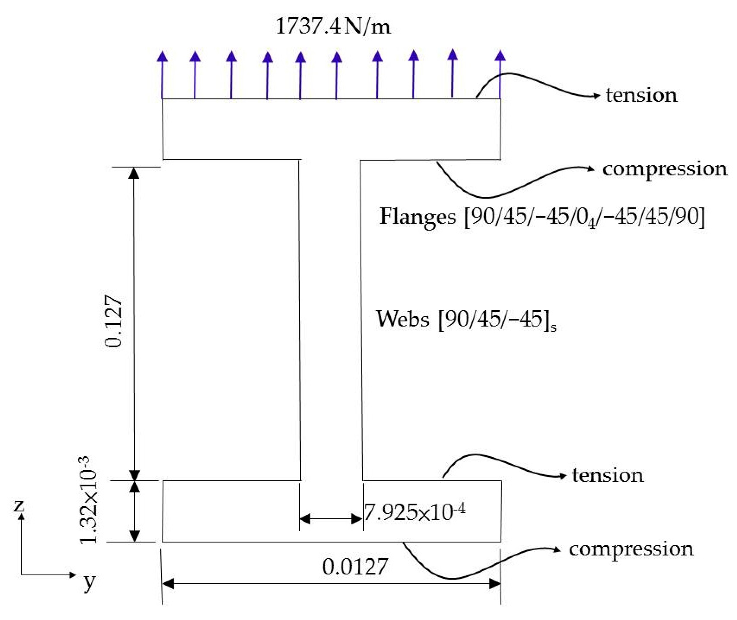
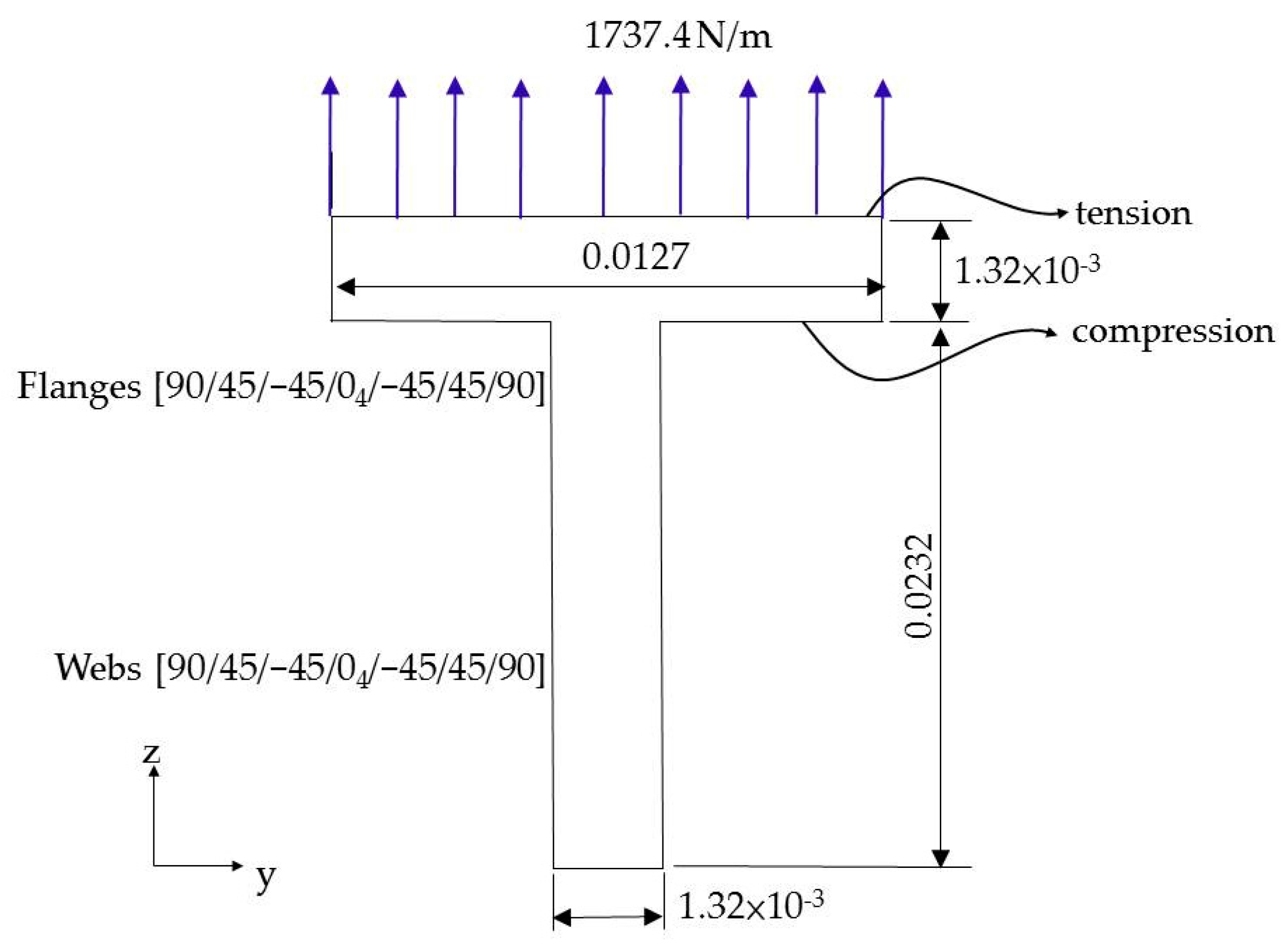
A simple support laminated composite T-beam, made of AS4/3501-6 carbon/epoxy, was divided into the web and flange to construct its geometric model. The web lamination sequence, symmetric flange lamination sequence, and non-symmetric flange lamination sequence were ${\left[90/45/-45\right]}_s$, ${\left[90/45/-45/0/0\right]}_s$, and $\left[0_4/90/45/-45/-45/45/90\right]$, respectively. The finite element software, MSC/NASTRAN, was used to analyze the composite laminated T-beam [29,30]. The material properties of the laminated plates include $E_{11}=1.27\times {10}^{11} \mathrm{GPa}$, $E_{22}=1.1\times {10}^{10} \mathrm{GPa}$, ${\upsilon }_{12}=0.28$, and $G_{12}=6.55\times {10}^9 \mathrm{GPa}$. The type of the element was set as the quadrilateral shell element of a 2D orthotropic. 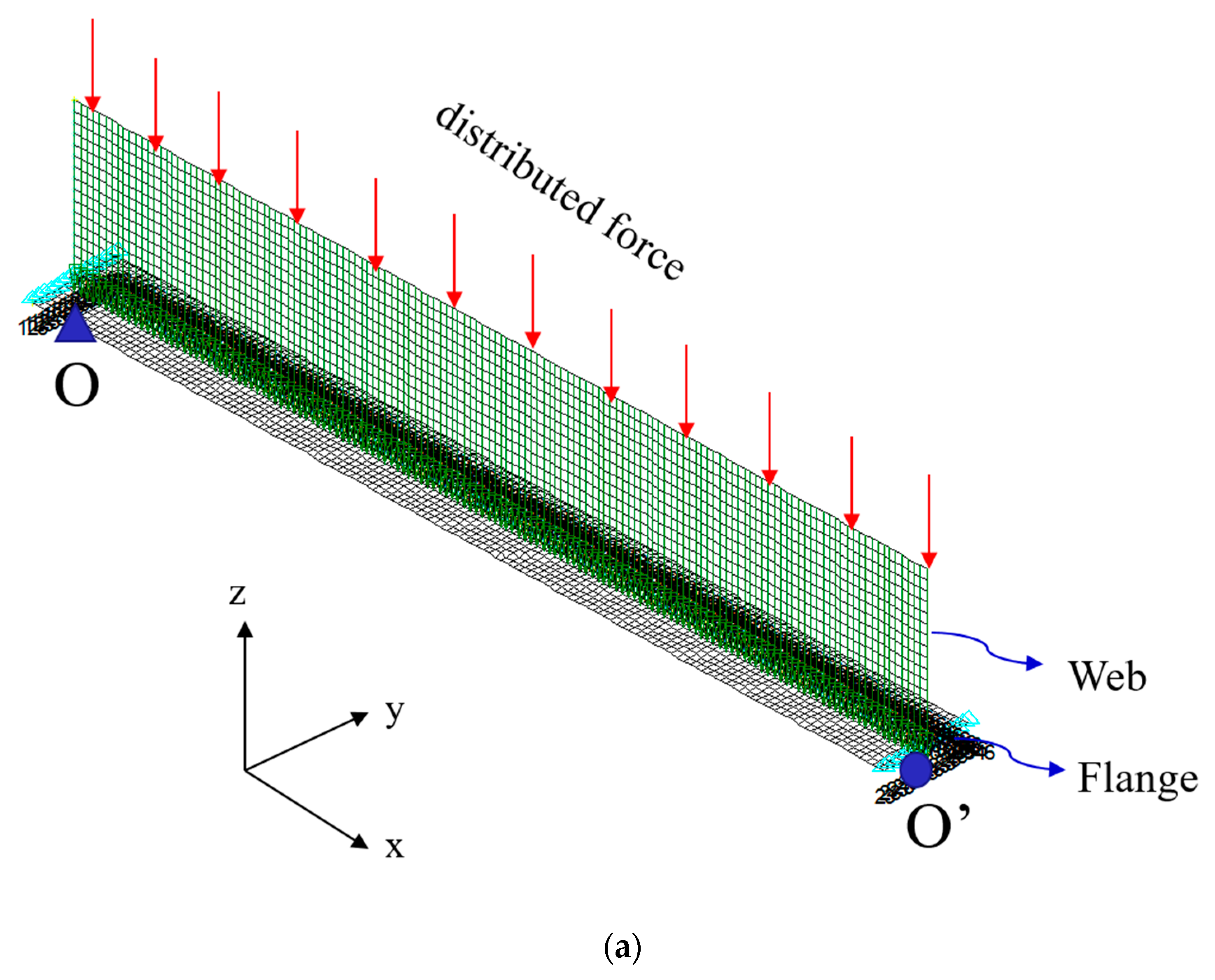The thickness of each laminate was $1.3208\times {10}^{-4}$ m. 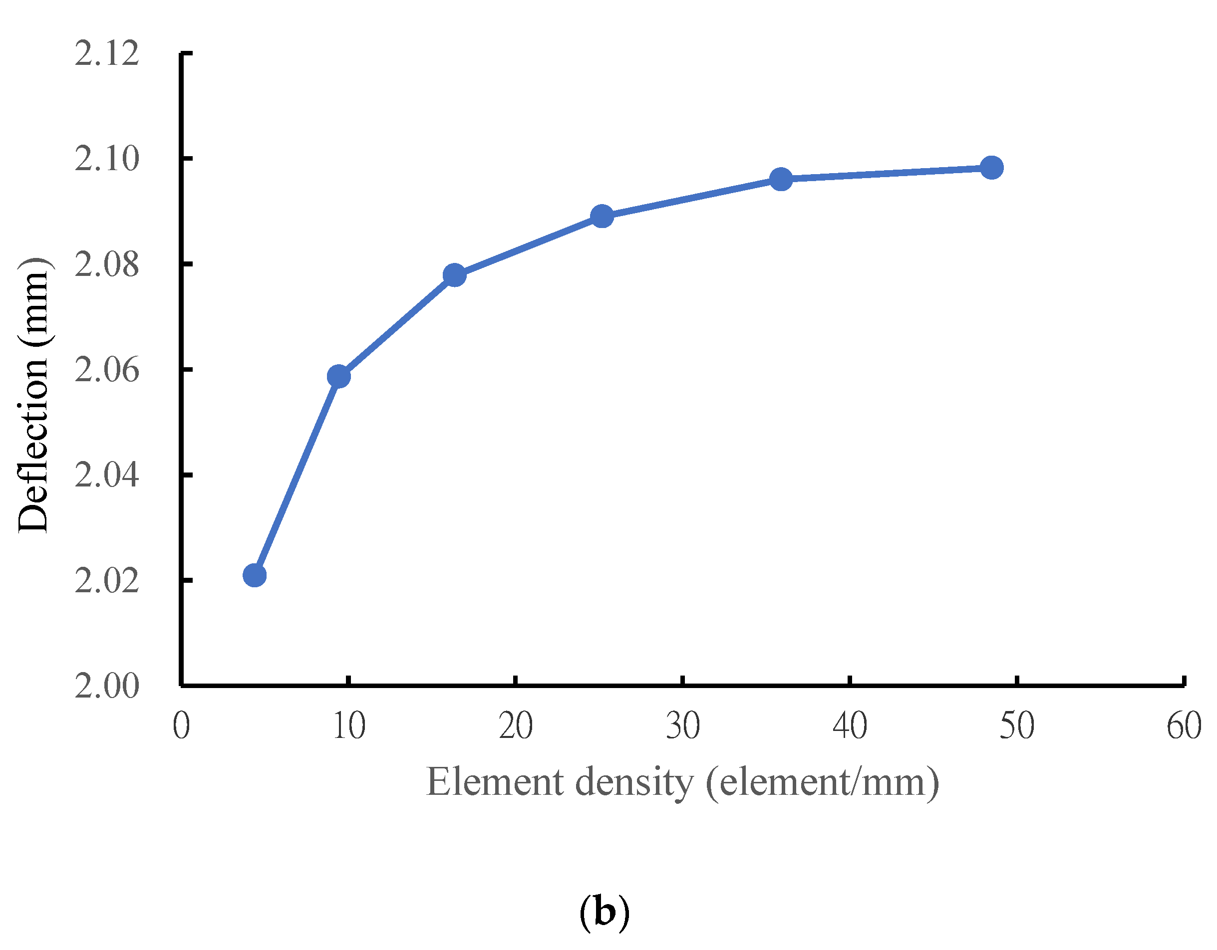The beam was a simple support structure whose web was subjected to a uniform force, as shown in Figure 3a. The point O boundary was set as the pin joint. The translational degrees of freedom were constrained in the x- and z-directions of the support points. The pin joints constrain the structure to the position of the support point; however, they allow the support point to rotate. In addition, the point O’ boundary was set to the roller joint. The nodes on the roller were only allowed to translate parallel to the roller support surface and allow the support point to rotate. The length of the beam, flange width, and web height were 0.127, 0.0127, and 0.01905 m, respectively. The beam was set as a simply supported beam with a length of 0.127 m at the boundary condition. A distributed force of 1737.4 N/m was applied to the web. The data convergence or divergence was determined by dividing the maximum deflection value obtained by different element densities in the FEM. The maximum deflection of the supported beam was observed to be located at the center of the beam. When the mesh density per unit length was set higher than 50 elements/mm, the deflection of the beam approached a convergent value, as shown in Figure 3b, where 12,600 elements and 13,051 nodes were used to achieve the highest accuracy in the FEM.

4. Results and Discussion

This section discusses the maximum deflection and bending stress of a simple supported laminated T-shaped composite beam subjected to a uniform distributed force. The theoretical solution was analyzed and compared with the FEM. The accuracy range of the beam-theory solution could be clearly defined based on the obtained results.

4.1. Theoretical Solution Error of Laminated Composite T-Beam

The theoretical and finite element analyses of symmetric and non-symmetric laminated composite T-beams are shown in Figure 4 and Figure 5, respectively. The deflection and stress, calculated using both methods, were compared at different aspect ratios of the beam. The results indicated that the theoretical solution of 1D used the Kirchhoff–Love hypothesis. Therefore, only the axial strain (${\epsilon }_x$) of the beam was considered in the theoretical derivation for 1D structures, whereas the plane (${\epsilon }_x$, ${\epsilon }_y$) and shear (${\gamma }_{xy}$) strains were considered in the derivation for the 2D structures. The data suggested that the aspect ratios less than 10 are not sufficiently accurate, owing to the increasing effect of the shear force on the deflection and stress with the decreasing beam length. Therefore, the theoretical formula for composite T-beams derived in this study is not suitable for short beams (L/h < 10). When the aspect ratio was higher than 10, the error curve tended to be flat and stable values were obtained for the bending stress and deflection. Therefore, the derived composite T-beam formula is accurate and suitable for thin and long beams.

4.2. Effect of Lamination Sequence and Geometry

The compressive resistance of the composite beams is poor. In the structure design, the compressive stress can be reduced using different arrangement sequences of the laminates or by changing the shape of the beam. In this study, the T- and I-shaped beams in the same lamination sequence were subjected to a uniform force and compared for stiffness, stress, and deflection. The cross-sectional views of the I- and T-shaped beams are shown in Figure 6 and Figure 7, respectively. The length, width, and height of the analyzed beam were 0.381, 0.0127, and 0.0127 m, respectively. The symmetrical flange and web of the I-shaped beam were laminated as ${\left[90/45/-45/0/0\right]}_s$ and ${\left[90/45/-45\right]}_s$, respectively. Both the web and flange laminates of the T-beam were ${\left[90/45/-45/0/0\right]}_s$. The height and width of the T-beam were 0.02032 m and 0.0127 m, respectively. Both beams were made of AS4/3501-6 carbon/epoxy, and the thickness of the laminate was $1.3208\times {10}^{-4}$ m. The material properties were $E_{22}=1.1\times {10}^{10} \mathrm{GPa}$, ${\upsilon }_{12}=0.28$, and $G_{12}=6.55\times {10}^9 \mathrm{GPa}$. Both beams were simply supported structures with a uniform upward force of 1737.4 N/m. The stress and deflection of the I- and T-beams were obtained using the derived theoretical composite T-beam solution and the I-shaped beam formula reported in the literature [31]. The data shown in

Table 1. Comparison of effective stiffness, stress, and deflection of beams.

	$\mathit{E}\mathit{I}{ (\mathbf{Nm}}^2)$	${\mathit{\sigma }}_{\mathit{t},\mathit{f}\mathit{l}\mathit{a}\mathit{n}\mathit{g}\mathit{e}} (\mathbf{GPa})$	${\mathit{\sigma }}_{\mathit{c},\mathit{f}\mathit{l}\mathit{a}\mathit{n}\mathit{g}\mathit{e}} (\mathbf{GPa})$	${\mathit{\delta }}_{\mathbf{max}} \left(\mathbf{m}\right)$
I-beam	677,028.69	$2.1169\times {10}^9$	$2.1169\times {10}^9$	0.004369
T-beam	793,457.28	$2.1202\times {10}^9$	$1.8822\times {10}^9$	0.003734
Difference (%)	+14.67	+0.156	−35.64	−14.53

suggests that when 0 laminations is added to the web and the height of the web is increased, the effective stiffness of the T-beam increases by 14.67% compared with that of the I-beam. Furthermore, the maximum deflection of the T-beam is observed to be 14.53% lower than that of the I-beam, thereby indicating that the fiber-reinforced composites can tolerate tensile stress better than they can tolerate compressive stress. The compressive stress of the T-beam on the lower layer of the upper flange is lower than that of the I-beam. The compressive stress on the flange is reduced by 35.64% because of the decrease in the distance between the centroid position of the T-beam and the centroid of the flange. The 0 laminations added to the web assist in increasing the effective stiffness of the beam.

5. Conclusions

The finite element analysis verified the assumptions made in deriving the theoretical model, and the applicable range of the proposed model could be determined. The following conclusions were drawn based on the results obtained from the theoretical analysis and finite element analysis:

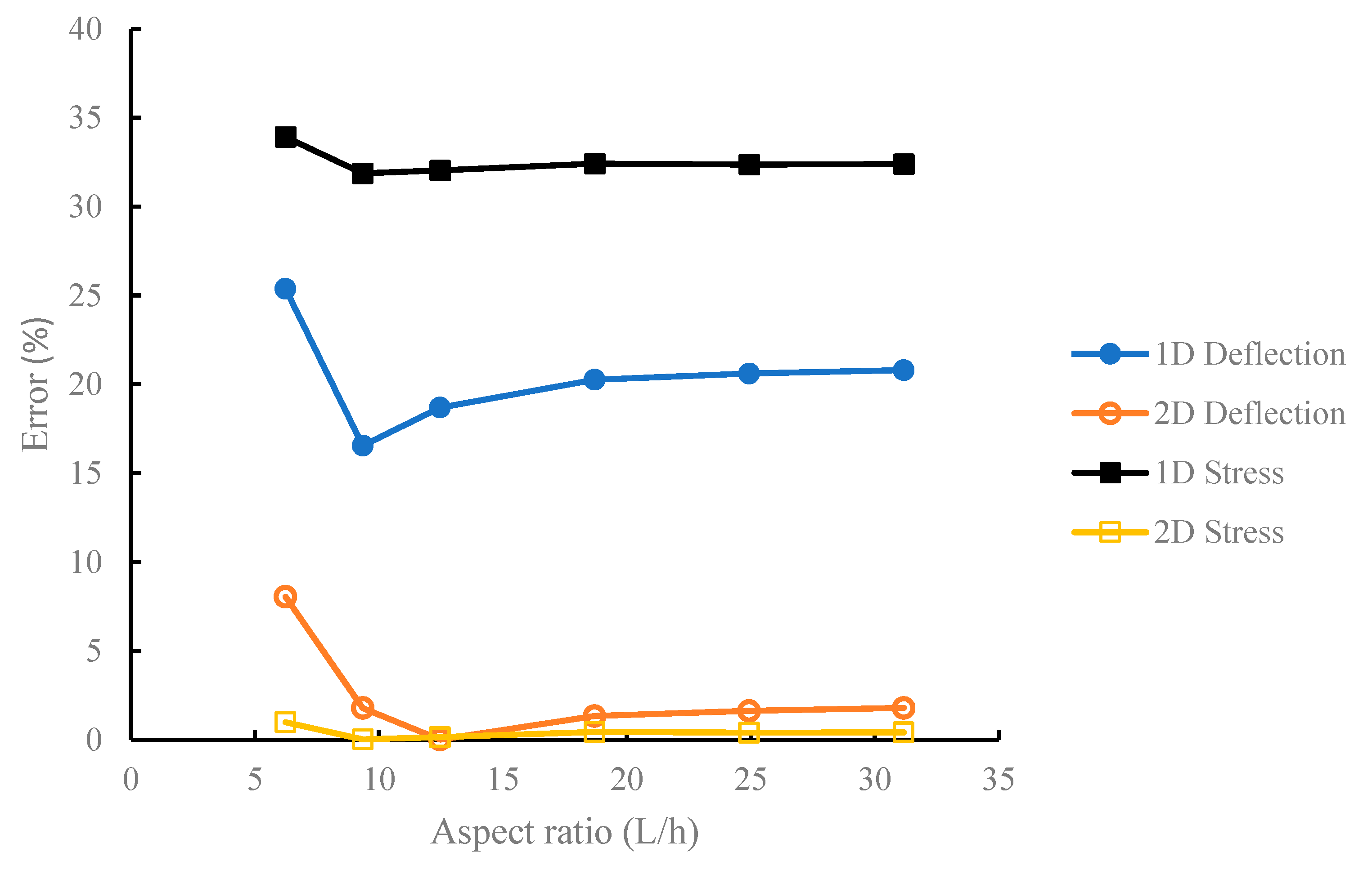
• The composite laminated T-beams were analyzed using 1D beam theory, and the centroid positions of the symmetric and non-symmetric T-beams were deduced. The 1D theoretical analysis was based on the Kirchoff-Love deformation hypothesis. Therefore, only the axial strain was considered. Consequently, the errors for deflection and stress were higher than 15%.
• The deflection and stress of the composite laminated T-beam were analyzed using 2D beam theory. The results suggested improvement in the accuracy of the 2D analytical solution when the aspect ratio was higher than 12. However, the accuracy was less than 2%. Therefore, the derived formula is considered applicable to slender beams.
• The effective stiffness of the laminated T-beam was 14.67% higher than that of the I-beam when the same material and lamination sequence was used in both structures. The higher effective stiffness is related to the higher bending moment owing to the location of the centroid of the T-beam closer to the flange. The addition of a 0 lamination to the web for a laminated T-beam increased the stiffness and reduced the flange compressive stress by 35.64%.
• The analytical solution for the laminated composite T-beam derived in this study is a fast and accurate theoretical method to calculate the deflection and bending stress of the composite beam.

This study investigated the accuracy and applicability of the derived bending stress, deflection, and effective stiffness of laminated composite T-beams. Among various engineering components, especially structures with anisotropic and geometric asymmetry, several issues have been discussed in the literature. Further, the bonding ability and life of each laminate are worth discussing in an environment of high temperature, thermal cycling, and torsion. This could be an important research area to explore in the future.