Author Contributions
Conceptualization, L.F.; Data curation, L.F. and S.D.; Formal analysis, H.S.; Methodology, L.F., H.S., V.P., S.D. and H.G.; Project administration, O.K.; Resources, O.K.; Software, L.F.; Supervision, O.K. and H.S.; Writing—original draft, L.F.; Writing—review & editing, L.F., H.S., V.P., S.D., H.G. and O.K. All authors have read and agreed to the published version of the manuscript.
Figure 1.
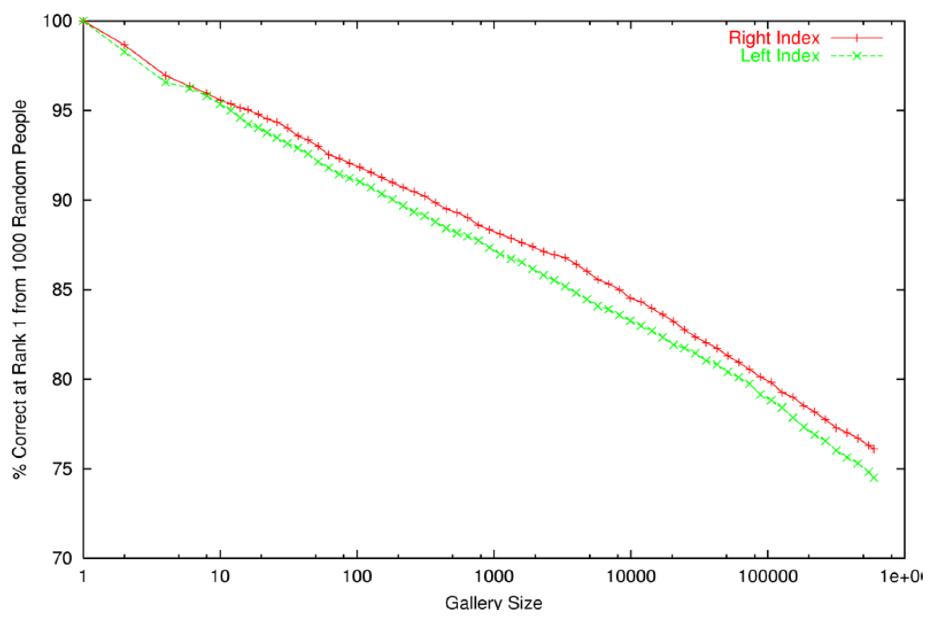
Probability of detection at Rank-1 IR as a function of more than 600,000 plain index fingers [
1] (See Figure 19). Note the log scale for the
x-axis. Probe set size was 1000 subjects. Fingerprint source: Department of Homeland Security, US Federal Government.
Figure 1.
Probability of detection at Rank-1 IR as a function of more than 600,000 plain index fingers [
1] (See Figure 19). Note the log scale for the
x-axis. Probe set size was 1000 subjects. Fingerprint source: Department of Homeland Security, US Federal Government.
Figure 2.
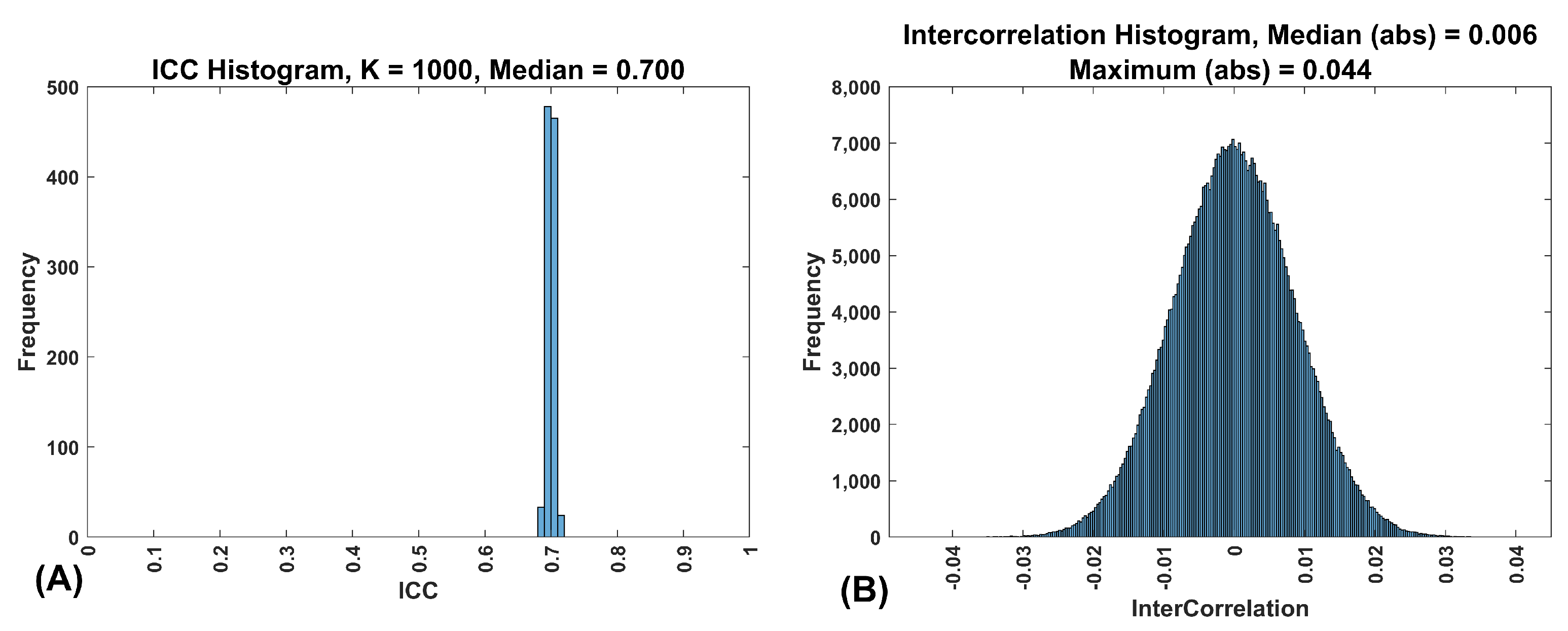
(A) Frequency histogram of ICCs for 1000 features with an . This was from a synthetic data set with 10,000 subjects. (B) Frequency histogram of correlations between 1000 features for 10,000 subjects, two sessions, with an . Note that the median and maximum are of the absolute value of the correlations.
Figure 2.
(A) Frequency histogram of ICCs for 1000 features with an . This was from a synthetic data set with 10,000 subjects. (B) Frequency histogram of correlations between 1000 features for 10,000 subjects, two sessions, with an . Note that the median and maximum are of the absolute value of the correlations.
Figure 3.
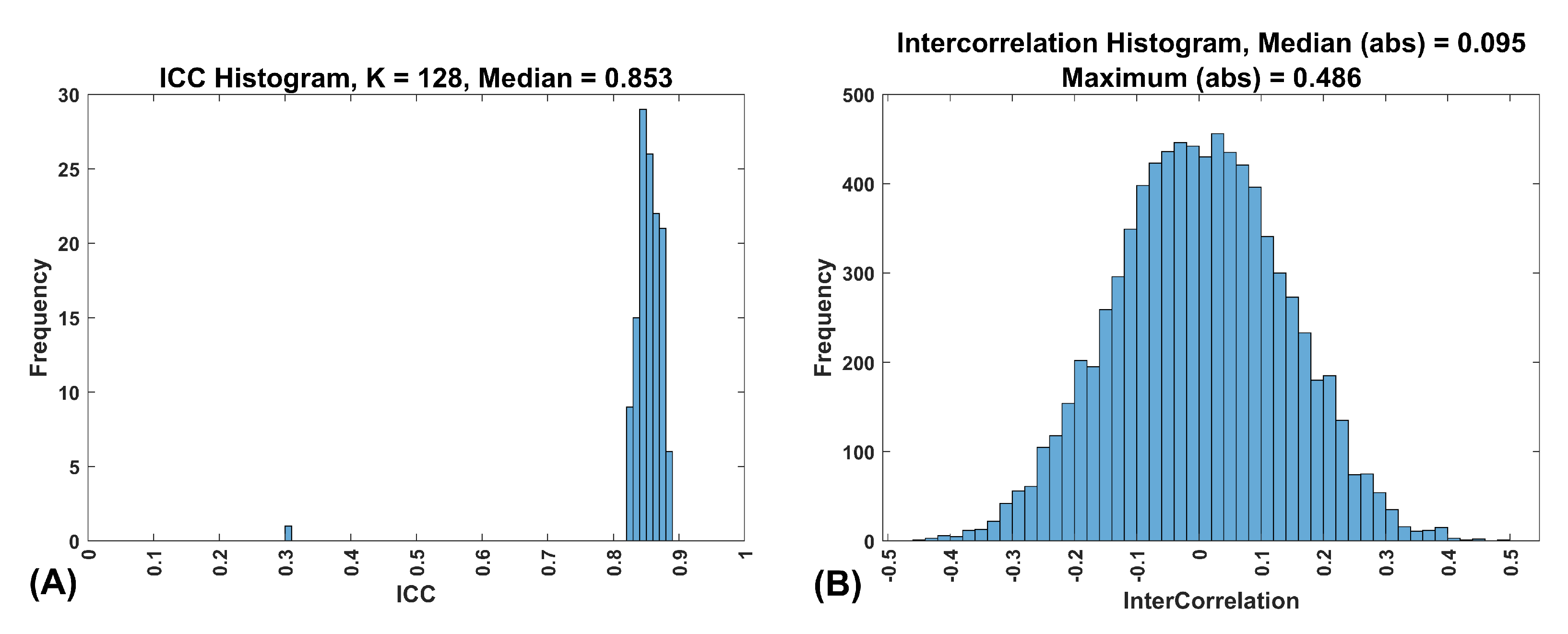
Characteristics of the FaceNet features. (A) This is a frequency histogram of the ICCs for the 128 FaceNet features. All of the features are between 0.8 and 0.9, which corresponds exactly with our synthetic Band 8 features. This indicates that these features are very reliable over time. (B) This is a frequency histogram of the intercorrelations of the 128 FaceNet features.
Figure 3.
Characteristics of the FaceNet features. (A) This is a frequency histogram of the ICCs for the 128 FaceNet features. All of the features are between 0.8 and 0.9, which corresponds exactly with our synthetic Band 8 features. This indicates that these features are very reliable over time. (B) This is a frequency histogram of the intercorrelations of the 128 FaceNet features.
Figure 4.
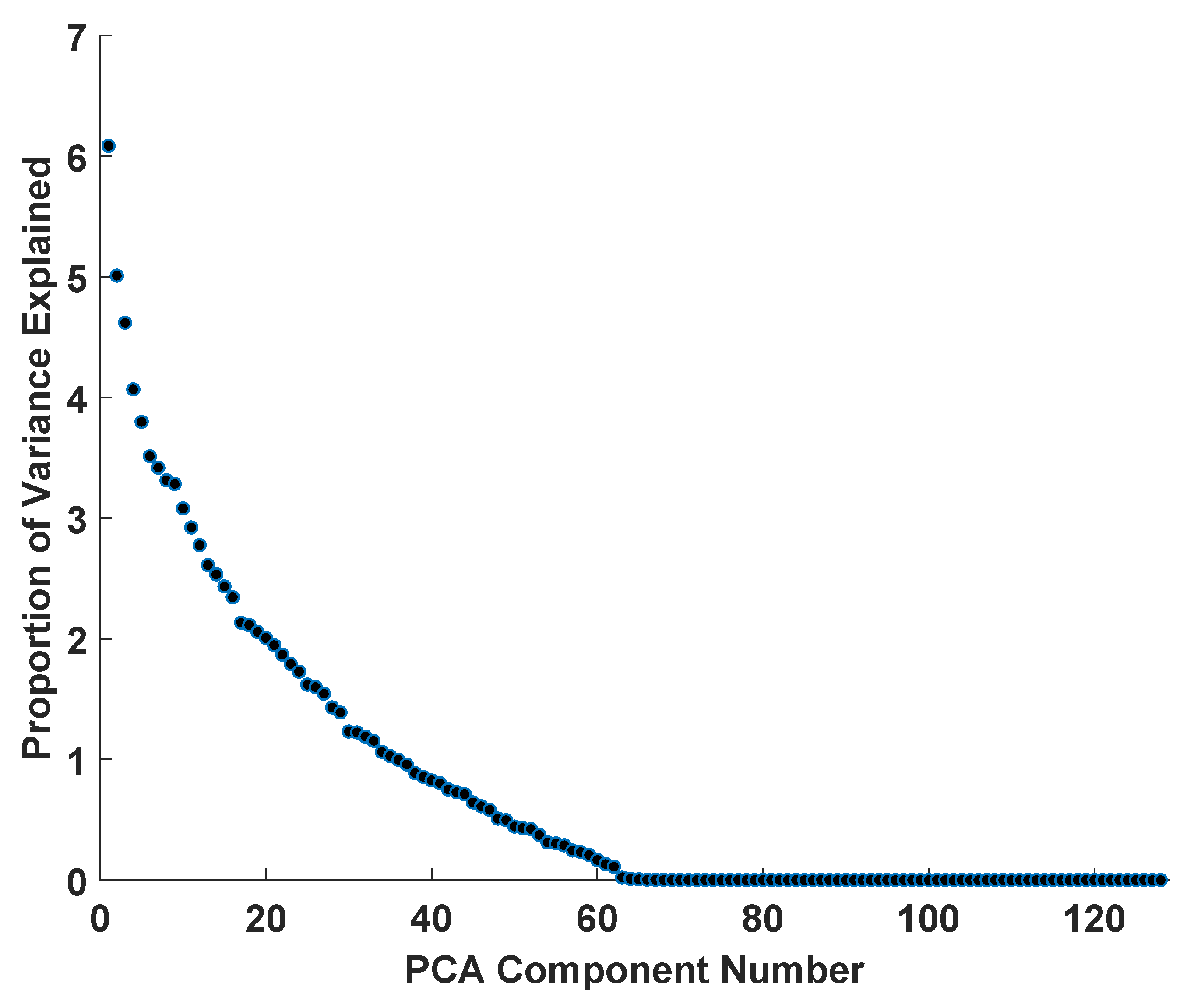
After PCA of the 128 FaceNet Features, we plot the variance explained by each PCA component against component number. Essentially all of the variance is accounted for by approximately 60 completely uncorrelated PCA components.
Figure 4.
After PCA of the 128 FaceNet Features, we plot the variance explained by each PCA component against component number. Essentially all of the variance is accounted for by approximately 60 completely uncorrelated PCA components.
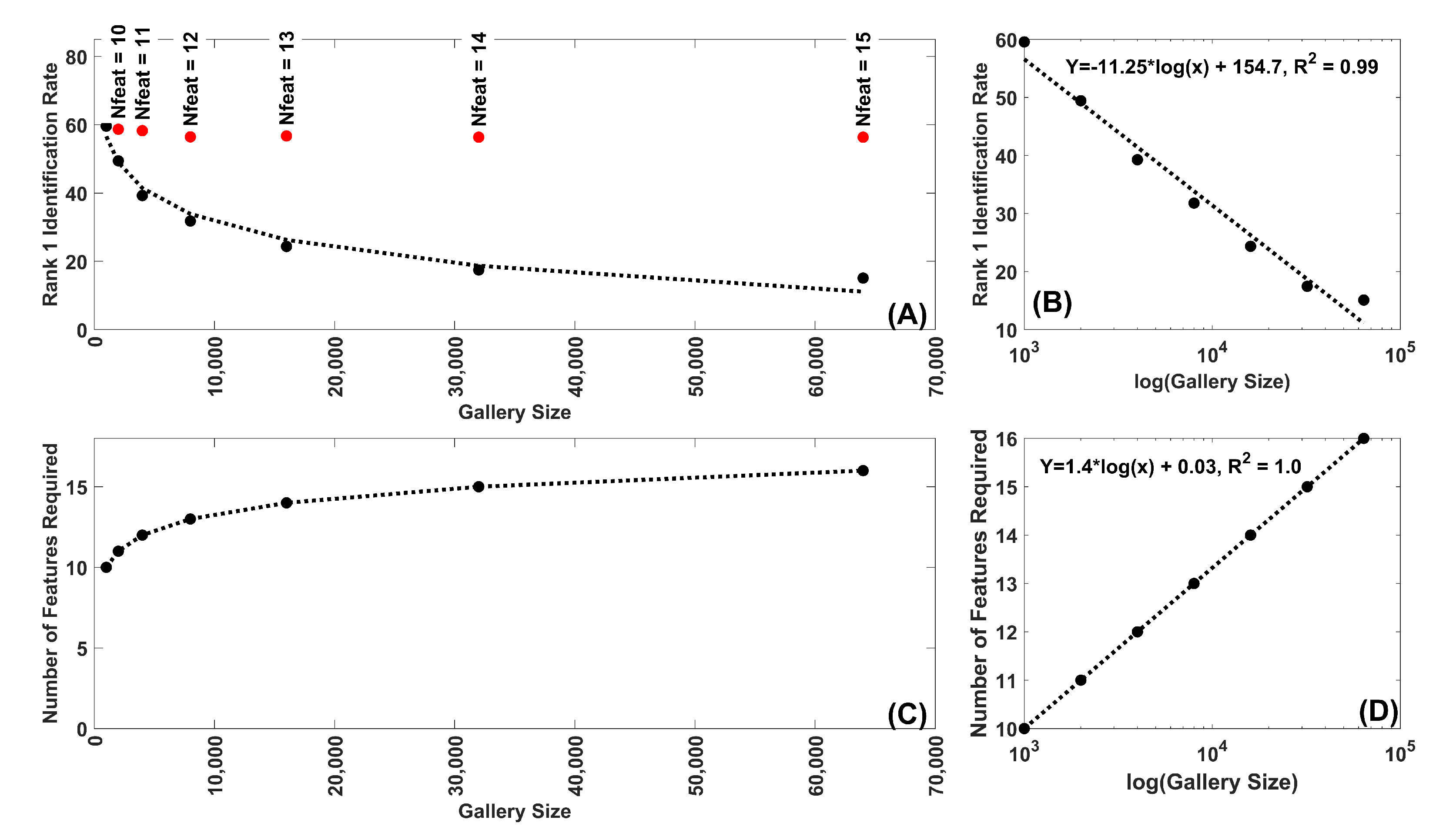
Figure 5.
(A) Rank-1 IR as a function of gallery size for synthetic Band 8 features. Each dot represents the mean of 30 repetitions. The black dots are the Rank-1 IR for 10 features for the following gallery sizes: 1000, 2000, 4000, 8000, 16,000, 32,000, 64,000 subjects. The red dots represent the Rank-1 IR for feature numbers greater than 10 which are chosen to produce a Rank-1 IR most similar to that for 10 features and 1000 subjects. (B) Same data as (A) plotted on a log(Gallery size) scale. Note the fit of the decline to a linear function of log(Gallery Size). (C) Plot of the number of features required for gallery sizes greater than 1000 to match the Rank-1 IR for 10 features, 1000 subjects. (D) Same data as (C) plotted on a log(Gallery size) scale. Note the fit of the increase to a linear function of log(Gallery Size). In this case a linear equation in log(Gallery Size) was able to match the results perfectly (r-squared = 1.0).
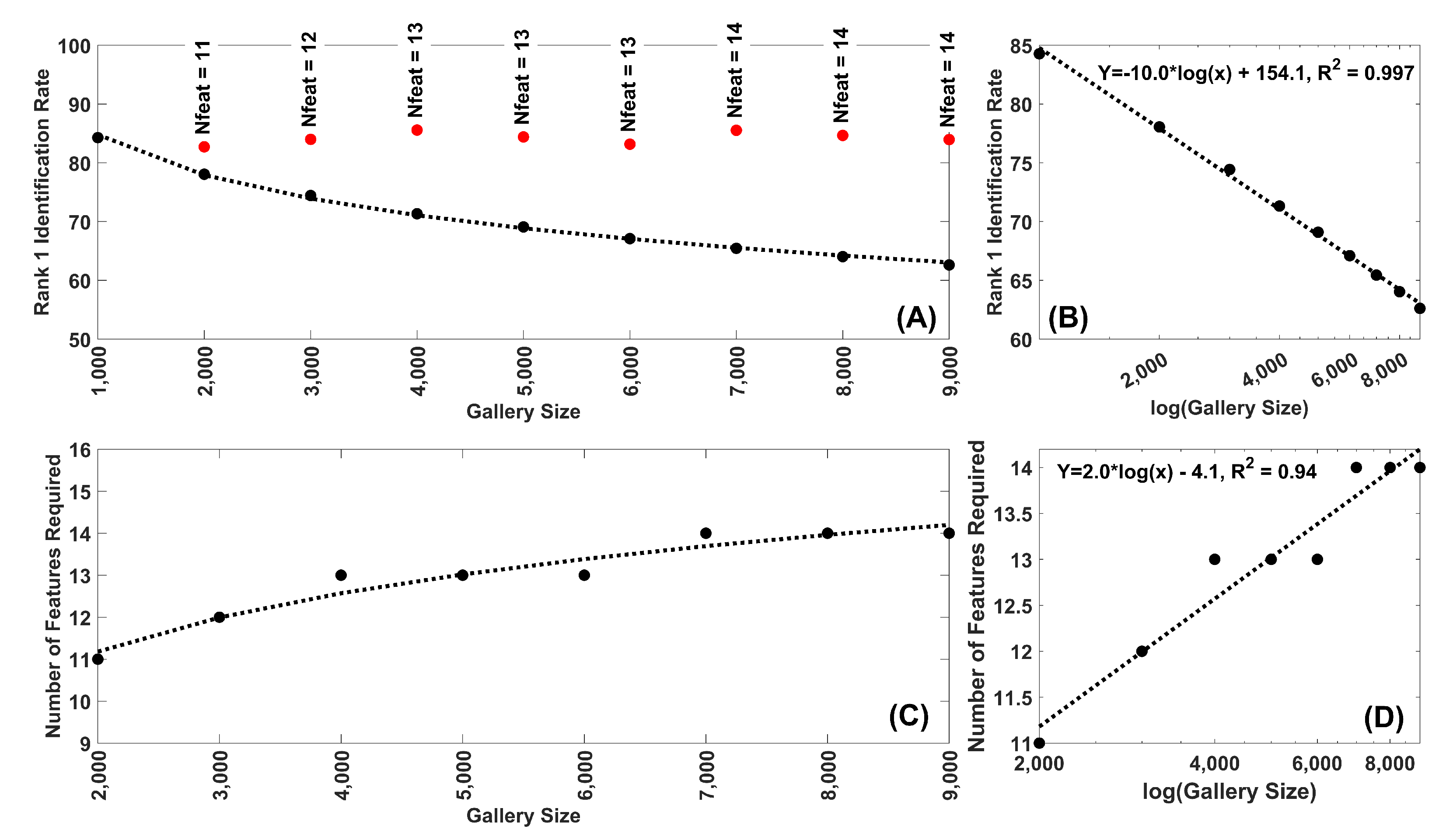
Figure 6.
(A) Rank-1 IR as a function of gallery size for FaceNet features. Each dot represents the mean of 30 repetitions. The black dots are the Rank-1 IR for 10 features for gallery sizes from 1000 to 9000 in 1000 size steps. The red dots represent the Rank-1 IR for feature numbers greater than 10 which are chosen to produce a Rank-1 IR most similar to that for 10 features and 1000 subjects. (B) Same data as (A) plotted on a log(Gallery size) scale. Note the fit of the decline to a linear function of log(Gallery Size), with an . (C) Plot of the number of features required for gallery sizes greater than 1000 to match the Rank-1 IR for 10 features, 1000 subjects. (D) Same data as (C) plotted on a log(Gallery size) scale. Note the fit of the increase to a linear function of log(Gallery Size). In this case a linear equation in log(Gallery Size) was able to match the results quite well ().
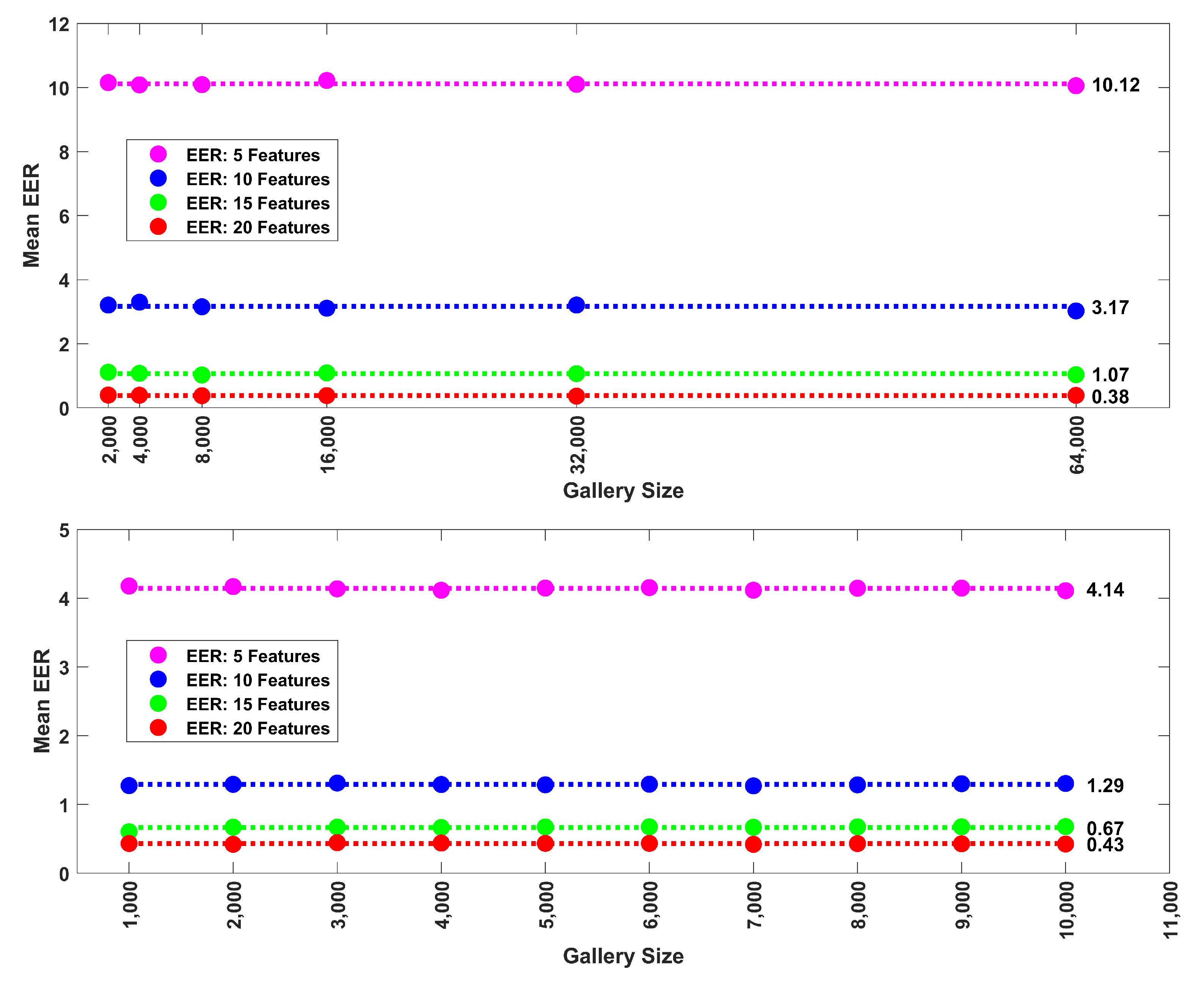
Figure 7.
(Top): Relationship between mean EER (30 repetitions) and gallery size for synthetic data (Band 8). Data shown for 5, 10, 15 and 20 features. The average EERs (shown to the right of the last dot) across gallery size are illustrated with dotted lines. Mean EER was highly stable with increases in gallery size. (Bottom): Relationship between mean EER (30 repetitions) and gallery size (1000 to 10,000 subjects in 1000 subject steps) for FaceNet PCA components. Data shown for the first 5, 10, 15 and 20 PCA components. The average EERs (shown to the right of the last dot) across gallery size are illustrated with dotted lines. Mean EER does not change as a function of gallery size.
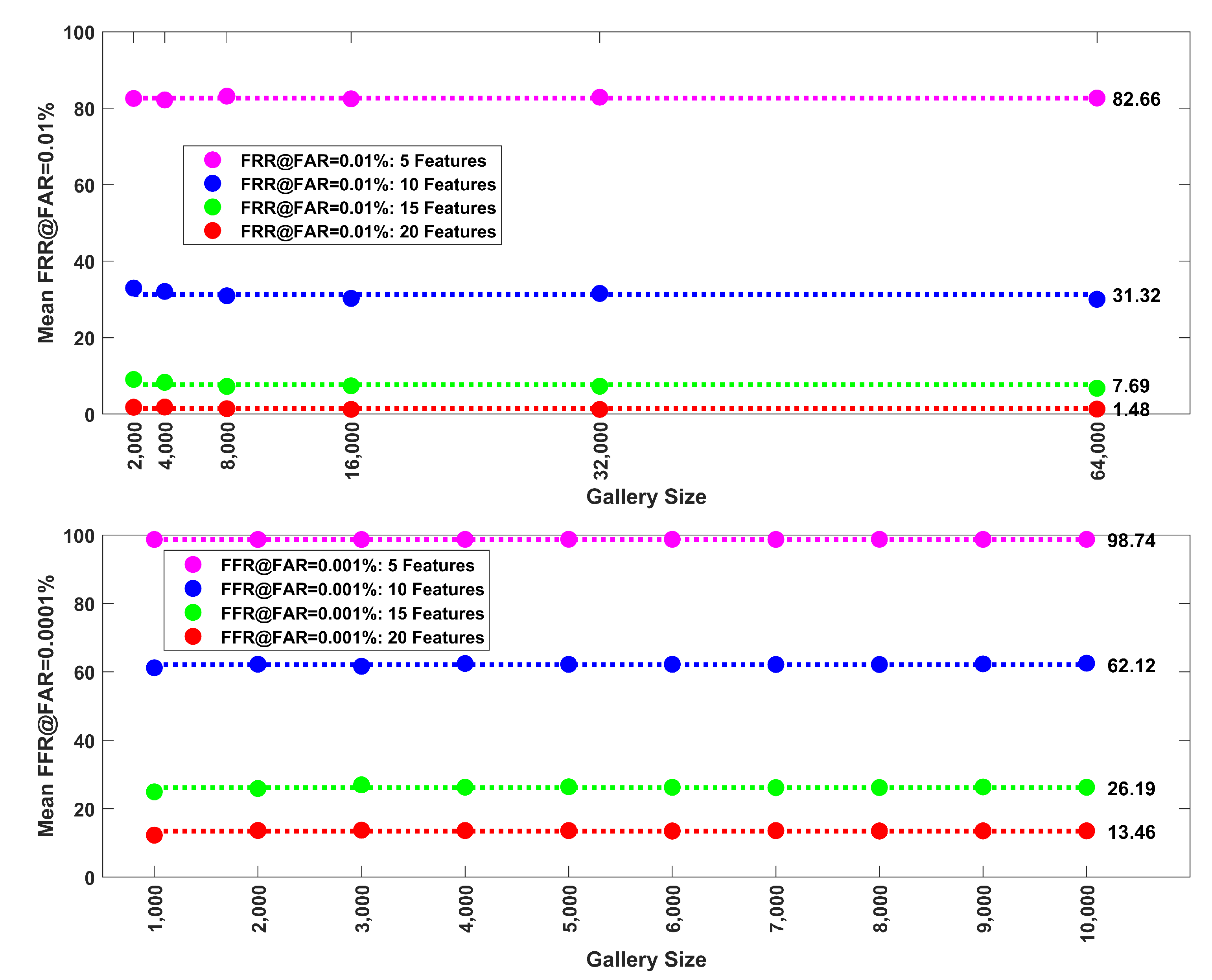
Figure 8.
(Top): In addition to mean EER, we also evaluated the mean false rejection rate (FRR) at a false positive rate of 0.01%. Here we plot these error rates (mean of 30 repetitions) versus gallery size (1000, 2000, 4000, 8000, 16,000, 32,000, 64,000 subjects) for synthetic data (Band 8). Data shown for 5, 10, 15 and 20 features. The average error rates (shown to the right of the last dot) across gallery size are illustrated with dotted lines. There was some instability at small gallery sizes, but otherwise, the mean error rate did not change as a function of gallery size. (Bottom): FRR at FAR = 0.0001%. Here we plot these error rates (mean of 30 repetitions) versus gallery size (1000 to 10,000 in steps of 1000 subjects) for FaceNet PCA components. Data shown for 5, 10, 15 and 20 PCA components. The average error rates (shown to the right of the last dot) across gallery size are illustrated with dotted lines. The mean error rate did not change as a function of gallery size.
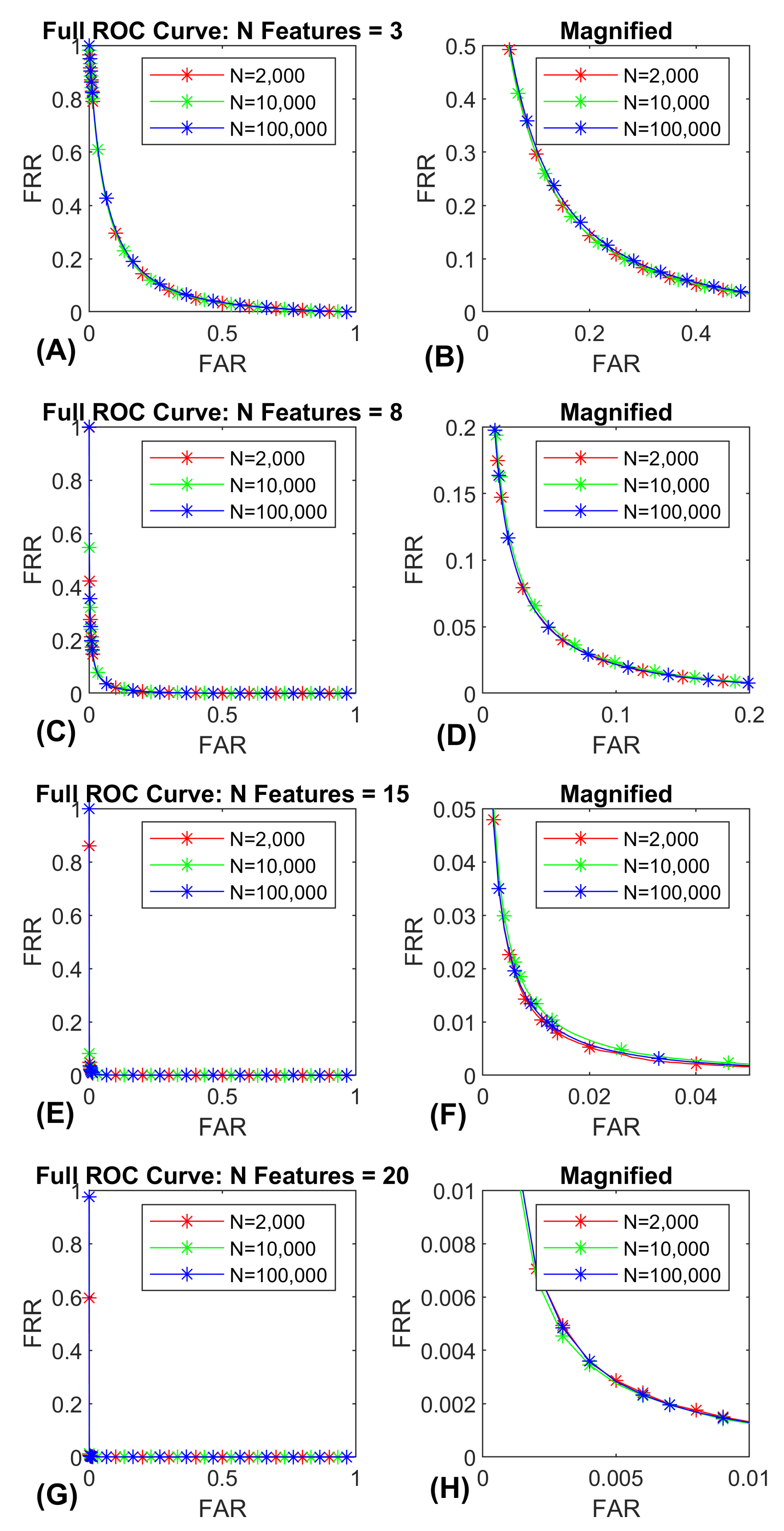
Figure 9.
ROC-curves for synthetic data (Band 8). Curves for 3, 8, 15 and 20 features. Each curve was evaluated at gallery sizes of 2000, 10,000 and 100,000 subjects. Each curve is the average over 30 repetitions. (A) illustrates the entire 3 ROC-curves for 3 features. (B) illustrates the same data in (A) zoomed in on the lower error rates for enhanced visibility. (C) illustrates the entire 3 ROC-curves for 8 features. (D) illustrates the same data in (C) zoomed in on the lower error rates for enhanced visibility. (E) illustrates the entire 3 ROC-curves for 15 features. (F) illustrates the same data in (E) zoomed in on the lower error rates for enhanced visibility. (G) illustrates the entire 3 ROC-curves for 20 features. (H) illustrates the same data in (G) zoomed in on the lower error rates for enhanced visibility. Note that the ROC-curves are essentially overlapping across gallery size.
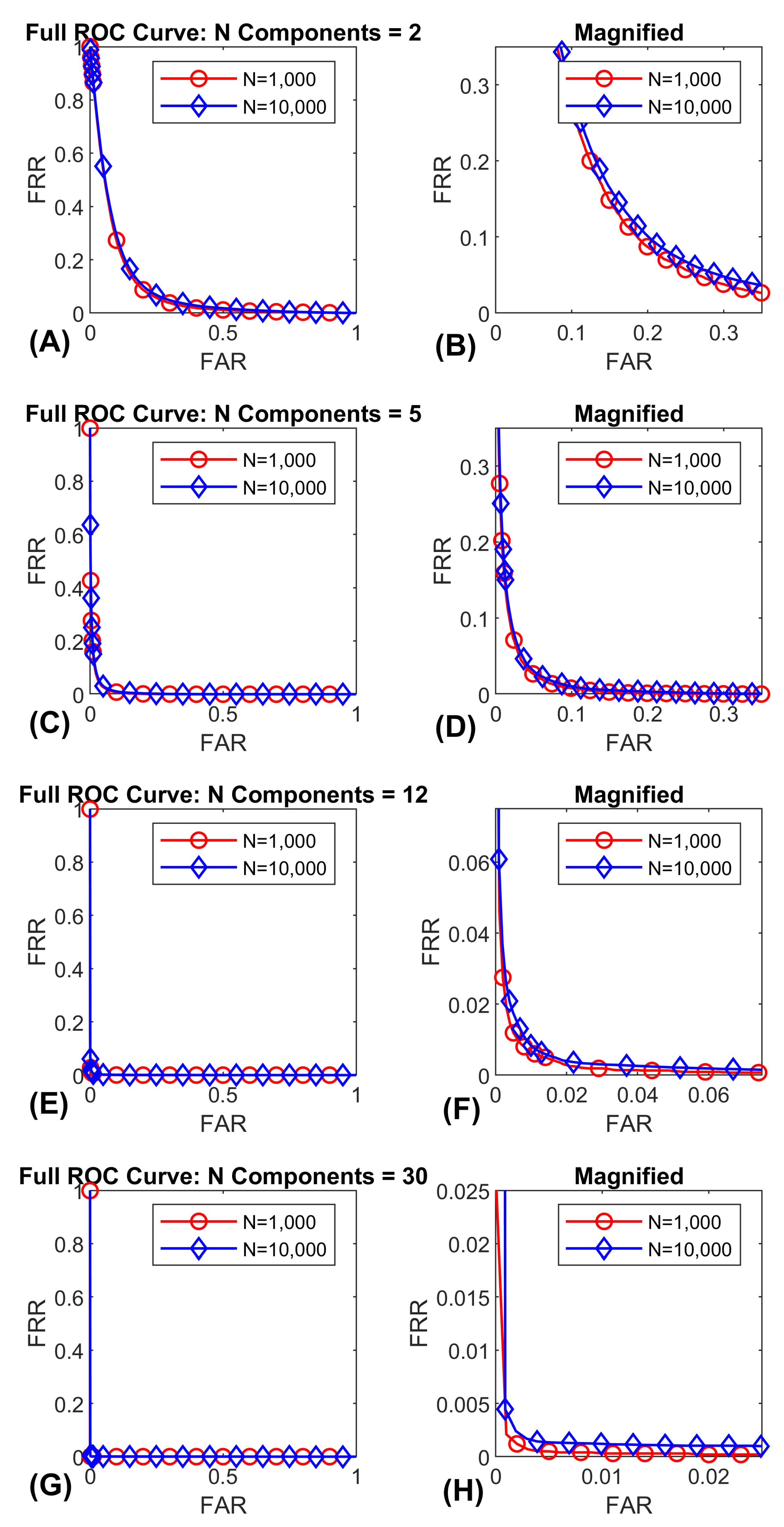
Figure 10.
ROC-curves for FaceNet PCA components. Plots for 2, 5, 12 and 30 PCA components are displayed. Each curve was evaluated at 1000 and 10,000 subjects. Each curve is the average over 30 repetitions. (A) illustrates the entire 2 ROC-curves for 2 features. (B) illustrates the same data in (A) zoomed in on the lower error rates for enhanced visibility. (C) illustrates the entire 2 ROC-curves for 5 features. (D) illustrates the same data in (C) zoomed in on the lower error rates for enhanced visibility. (E) illustrates the entire 2 ROC-curves for 12 features. (F) illustrates the same data in (E) zoomed in on the lower error rates for enhanced visibility. (G) illustrates the entire 2 ROC-curves for 30 features. (H) illustrates the same data in (G) zoomed in on the lower error rates for enhanced visibility. Note that the ROC-curves are essentially overlapping across gallery size.
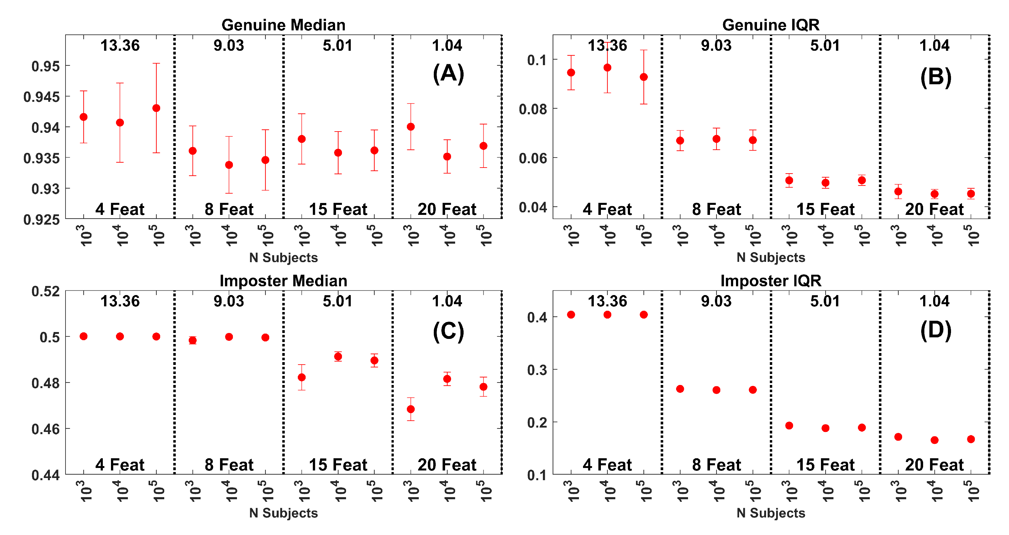
Figure 11.
(A) Median of the genuine similarity score distributions for synthetic data. Data are for the Band 8 data set with 4, 8, 15 and 20 features. Each dot is based on 30 repetitions. The error bars are at . The numbers at the top of each plot are the average EERs across the gallery sizes represented. (B) IQR of the genuine similarity score distributions for the same data in (A). (C) Median of the impostor similarity score distributions. (D) IQR of the impostor similarity score distributions.
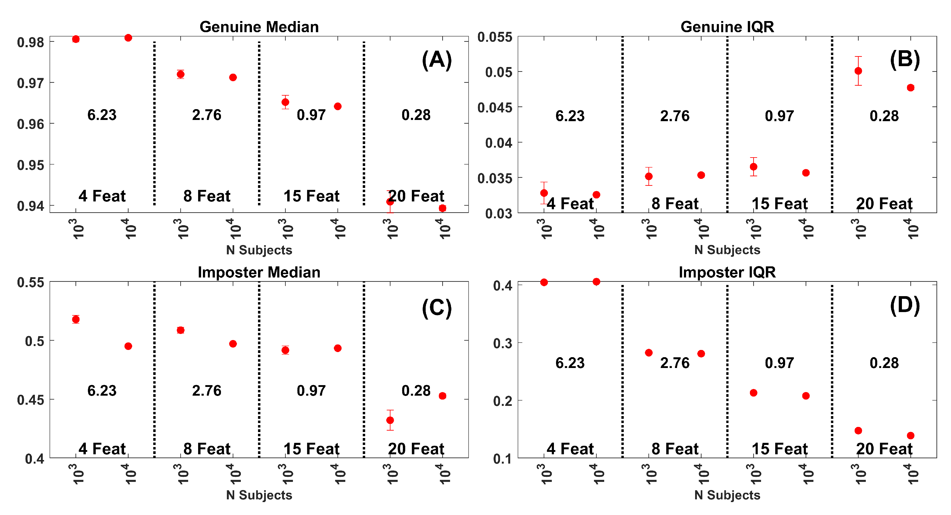
Figure 12.
(A) Median of the genuine similarity score distributions for the FaceNet PCA Components. Results for 4, 8, 15 and 20 PCA components. Each dot is based on 30 repetitions. The error bars are at . The numbers in the middle of each plot are the average EERs across the gallery sizes represented. (B) IQR of the genuine similarity score distributions for the same data in (A). (C) Median of the impostor similarity score distributions. (D) IQR of the impostor similarity score distributions.
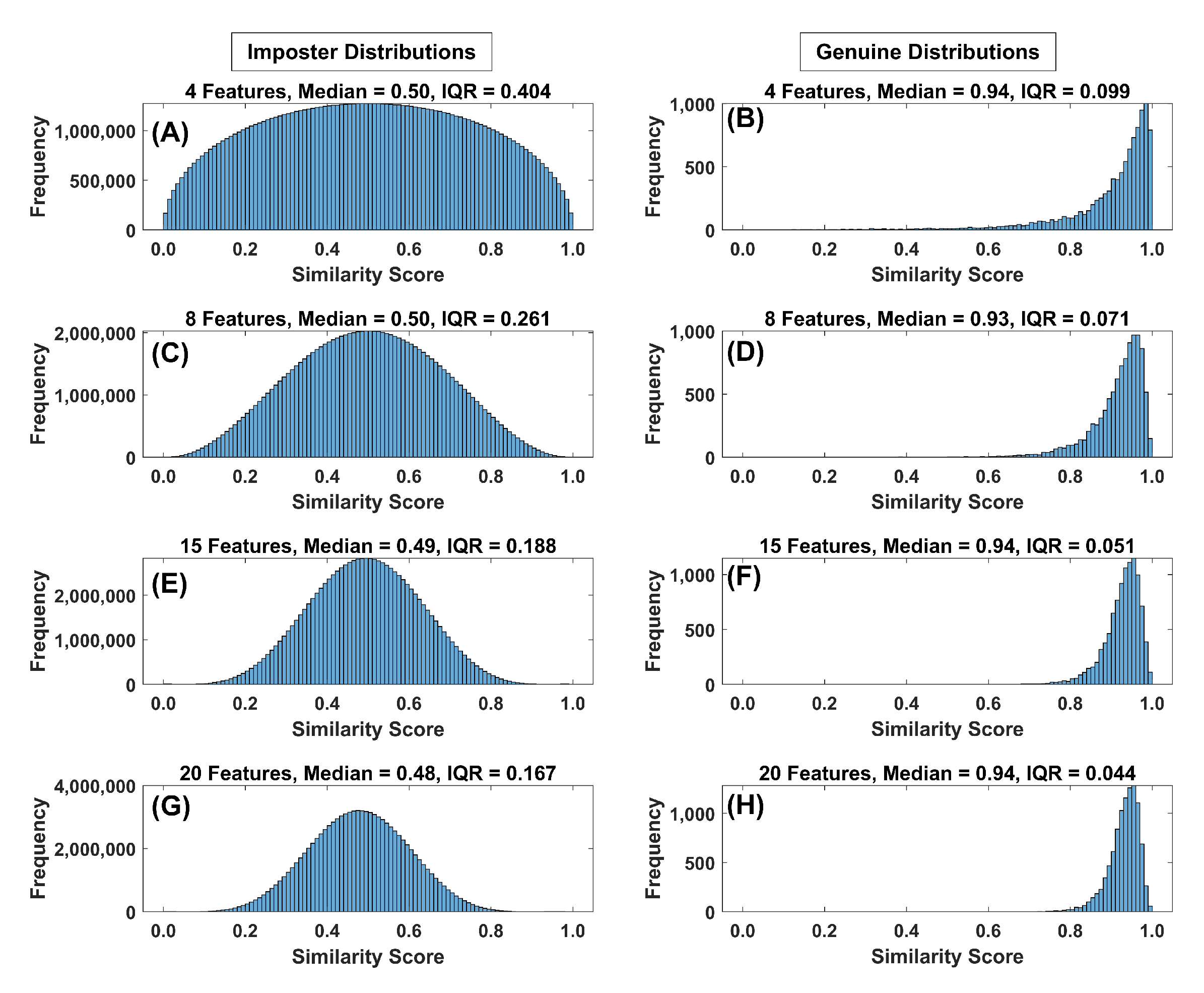
Figure 13.
(A) Histogram of the impostor similarity score distribution for synthetic data (4 features, Band 8 (all histograms), 10,000 subjects (all histograms)). Note the median and IQR value just above the histogram. (B) Histogram of the genuine similarity score distribution for 4 features. (C) Histogram of the impostor similarity score distribution for 8 features. (D) Histogram of the genuine similarity score distribution for 8 features. (E) Histogram of the impostor similarity score distribution for 15 features. (F) Histogram of the genuine similarity score distribution for 15 features. (G) Histogram of the impostor similarity score distribution for 20 features. (H) Histogram of the genuine similarity score distribution for 20 features.
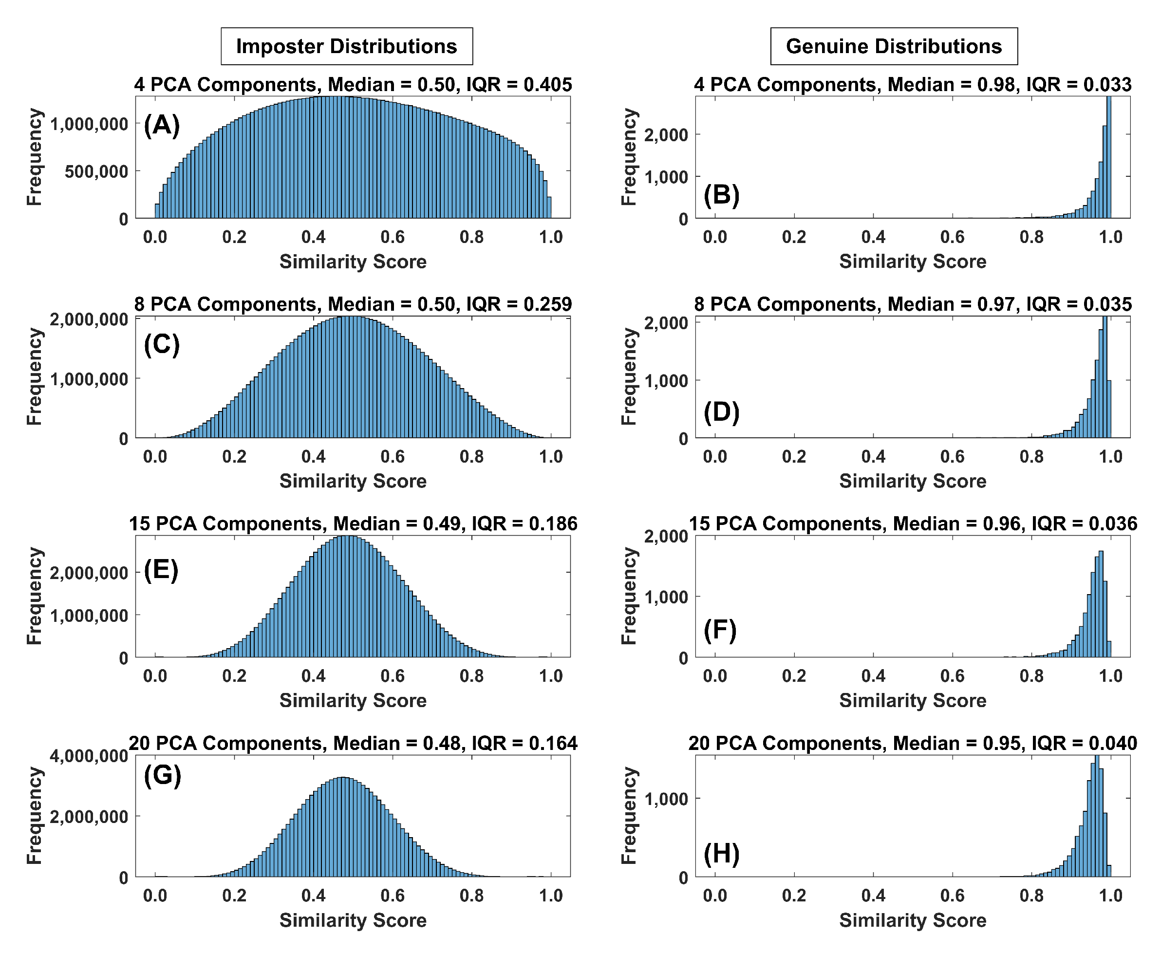
Figure 14.
(A) Histogram of the impostor similarity score distribution for FaceNet PCA components (4 PCA components, 10,000 subjects (all histograms)). Note the median and IQR value just above the histogram. (B) Histogram of the genuine similarity score distribution for 4 PCA components. (C) Histogram of the impostor similarity score distribution for 8 PCA components. (D) Histogram of the genuine similarity score distribution for 8 PCA components. (E) Histogram of the impostor similarity score distribution for 15 PCA components. (F) Histogram of the genuine similarity score distribution for 15 PCA components. (G) Histogram of the impostor similarity score distribution for 20 PCA components. (H) Histogram of the genuine similarity score distribution for 20 PCA components.
Table 1.
Summary of Major Results.
Table 1.
Summary of Major Results.
| Rank-1 IR decreases in a log-linear fashion with increasing gallery sizes |
| EER was stable across gallery sizes. |
| The false rejection rate at several false positive rates was also stable |
| across gallery sizes. |
| The shape of the ROC-curves was not affected by the gallery size. |
| The largest change among the 4 metrics (median genuine, IQR genuine, |
| median impostor and IQR impostor), as biometric performance improves, |
| was for the IQR of the impostor similarity score distribution. |

 ,
, 


