Article

Prediction Method for Mine Earthquake in Time Sequence Based on Clustering Analysis

School of Mines, China University of Mining and Technology, Xuzhou 221116, China
*
Author to whom correspondence should be addressed.
Appl. Sci. 2022, 12(21), 11101; https://doi.org/10.3390/app122111101
Submission received: 21 September 2022 / Revised: 27 October 2022 / Accepted: 31 October 2022 / Published: 2 November 2022
(This article belongs to the Special Issue Mechanical Properties of Rocks under Complex Stress Conditions)

Abstract

:
Under the background of the intelligent construction of a coal mine, how to efficiently extract effective information from the massive monitoring data of mine earthquakes, and improve prediction accuracy, is a research hotspot in the field of coal mine safety production. In view of this problem, more and more machine learning methods are being applied to the prediction on mine earthquakes. Considering that clustering analysis can enhance the correlation between microseism data, we propose a method whose main idea is to cluster microseism data before establishing the prediction model, and then train the model, so as to improve prediction accuracy. Specifically, microseism events on a working face are divided into clusters in advance by the Spatial Temporal-DBSCAN(ST-DBSCAN) algorithm, then a prediction model is established with Support Vector Regression (SVR) to predict the occurrence location and daily frequency of high-energy mine earthquake events. A set of engineering experiments were conducted in H Coal Mine, and the results show that the spatial-temporal clustering analysis of microseism events can indeed improve the prediction accuracy of machine learning methods on mine earthquakes.

1. Introduction

A mining induced earthquake refers to the seismic activity caused by surface or underground mining, which is referred to as a mine earthquake [1]. The mine earthquake is an abnormal state of instability in the stress field of the surrounding rock in the mining process. It is manifested as the vibration of coal and rock mass, caused by the sudden release of local elastic energy, which can be caused by the destruction of local ore bodies, such as spalling rib, rock burst, etc., or the sliding activity of faults. In recent years, with the increase of mining depth and the mining intensity of coal resources in China, the phenomenon of mine earthquake has begun to show up with unprecedented frequency, intensity, and complexity. Strong mine earthquakes have occurred in many mining areas across the country (the maximum magnitude is 3.1). In the Ordos mining area alone, in 2021 there were six 2.0 magnitude or above mine earthquakes [2], leading to mine earthquake becoming a sensitive topic, and even causing social panic. Strong mine earthquake activities are not only easy to cause dynamic disasters such as underground rock bursts [3], but also cause consequences such as ground shaking, collapse, and building damage [4]. Therefore, it is necessary to carry out monitoring and early warning research on the mine earthquake phenomena.
Since the 1990s, microseism monitoring technology has been widely used in the monitoring and early warning of mine earthquakes by coal mining enterprises, due to its advantages of high sensitivity and strong practicability [5]. In mining and production, the dynamic and static loads cause the deformation and instability of the coal and rock mass, or else the geological fault, fold, and other defective structures, are activated to trigger geological activities, which will release vibration waves with different frequencies and energy levels. The principle of the microseism monitoring system is to capture the relevant information of seismic waves, and determine the spatial-temporal location of the source, the strength and frequency of microseism activities, and other high-energy release activity information through calculation and inversion [6]. At present, microseism monitoring technology has made great progress in station network optimization, seismic wave pickup, inversion positioning, and waveform real-time monitoring, and has made a series of important research achievements [7]. The microseism monitoring system can identify the micro vibration wave and its dynamic change process in the whole coal mine, obtain the specific information of the time, space, and intensity of the microseism event, and directly reflect the real-time mechanical characteristics evolution of the coal mine.
With the increasingly mature and extensive application of microseism monitoring technology, it has become an effective means for the early warning of coal mine disasters, such as rock burst. It works by using a large amount of microseism monitoring data to analyze the breaking and migration laws of coal seam mining surrounding rocks, and to summarize the spatial scale, combined structure, the mechanical parameters of key stratum, and the correlation between the breaking process and high-energy microseism events. He et al. [8] used microseism monitoring technology to analyze the temporal and spatial evolution law of microseism events before and after the breaking of key stratum, laying a foundation for the prediction on rock burst using the combination of strata movement theory and microseism monitoring technology. Yuan et al. [9] analyzed the time sequence characteristics of microseism signals during the period of rock burst, and then obtained the spectrum characteristics and distribution change laws of microseism signals. Wang et al. [10] analyzed the waveform signals of microseism events and obtained the power spectrum evolution characteristics before and after the occurrence of rock burst. Xiao et al. [11] revised the maximum effective amplitude based on the attenuation characteristics of microseism waves in deep buried tunnels, taking the relative effective amplitude and the maximum effective frequency as spectrum analysis parameters. Wei et al. [12] analyzed the time-domain waveform and frequency spectrum characteristics of microseism signals when rock burst occurred in the coal mine by using the fast Fourier transform method. Peng [13] classified the microseism signal categories of coal mine working faces and analyzed the distribution law of microseism events in time and space. However, in the face of microseism monitoring signals containing a large amount of information, it is difficult to manually define and extract parameters to reflect all the features of microseism events, which makes it easy to cause a large amount of effective information to be ignored. As a result, current microseism monitoring can only monitor and reflect the microseism events that have occurred, and are occurring, and it is difficult to accurately judge the potential microseism events that may occur.
Traditionally, mine earthquake prediction usually uses geophysical methods to monitor some precursory signals, and the synthetic index method with artificially defined and extracted parameters is used to evaluate the possibility of the occurrence of high-energy mine earthquakes. The determination of the index and corresponding weight involves subjectivity and inconsistency. Machine learning can well overcome the problems caused by the synthetic index method. Its modeling process does not involve too much subjective decision-making, and is a data-driven strategy. Using the machine learning model, researchers do not need to pay attention to the weight of each index and the corresponding classification standard, they just need to know the specific value of each index, which is objective and measurable. At the same time, the use of intelligent devices such as microseism monitoring systems will generate massive real-time data carrying effective information. Empirically driven and mechanistically driven mine earthquake prediction methods are not enough to use these data, resulting in the loss of effective information. Using a data-driven method to solve the problem of mine earthquake prediction will become a breakthrough point for data-driven systems to enter the traditional engineering field, and is also a key step for mining to enter the smart mine and data mine era.
After the great development of computer hardware and the upsurge of machine learning, researchers continue to try to use data-driven methods, such as machine learning, to predict and warn of mine earthquake, achieved good results. Using the machine learning method to analyze microseism monitoring signals can get the most effective information, most of which cannot be obtained by an explicit algorithm. The machine learning method also has unique advantages in establishing the relationship between monitoring parameters and the time, location, and intensity of a mine earthquake. It can analyze the automatic monitoring signal into a high-dimensional matrix, without the need to manually determine the type of extraction parameters, and maximize the retention of signal features. Vallejos and Dong [14,15] established a logistic regression model to identify microseism events and mining blasting activities, respectively, with a higher accuracy than other analogy models. Del [16] established two neural network models to identify microseism events, one of which is used to extract signal features to construct training samples, and the other is used for event classification. In addition, machine learning methods such as random forest [17], Bayesian network [18], and support vector machine [19,20], are widely used for monitoring microseism events. However, these studies do not consider the spatial-temporal aggregation and activity correlation of microseism events, and the prediction accuracy of mine earthquake is not high; there is a lot of room for improvement. Microseisms are not isolated events. Mine earthquakes caused by a stress release usually have a similar spatial location, short time interval, and have the law of time series. If we first cluster the microseism data and then use the machine learning method to establish the prediction model, we will get better results.
Therefore, we propose to combine clustering analysis and machine learning methods to predict the high-energy mine earthquake in time sequence, including the occurrence location prediction and energy frequency prediction. In the selection of clustering algorithm, considering that microseism events include space and time information, the ST-DBSCAN algorithm [21] is selected to cluster the microseism events occurring in the working face. After clustering, there are no large number of microseism events in a single cluster, so SVR [22], which is suitable for a small sample data set, is used to predict mine earthquakes in sequence [23,24]. As a comparison experiment, the number of microseism events included in the working face is large before clustering, so Long Short-Term Memory (LSTM) [25] with a good prediction effect of time series on a large sample data set is selected to predict mine earthquake [26].
The main contributions of this paper are summarized as follows.
(1) A time sequence prediction method for mine earthquake based on ST-DBSCAN using SVR is proposed. Clustering analysis can source microseism clusters and enhance the correlation of microseism data. This data preprocessing method can improve the accuracy of subsequent machine learning prediction models.
(2) Contrast engineering experiments in the H Coal Mine are conducted to evaluate the performance of the proposed method. The results show that, compared with the classical time sequence prediction method (LSTM) on unclustered microseism data, the SVR model has a better prediction effect of mine earthquake on clustered microseism data.
The remainder of this paper is organized as follows. The related machine learning algorithms are introduced in Section 2. The proposed approach is described in Section 3. A real case study is illustrated in Section 4. Conclusions and future work are summarized in Section 5.
2. Methodology Background

2.1. Spatial Temporal-DBSCAN

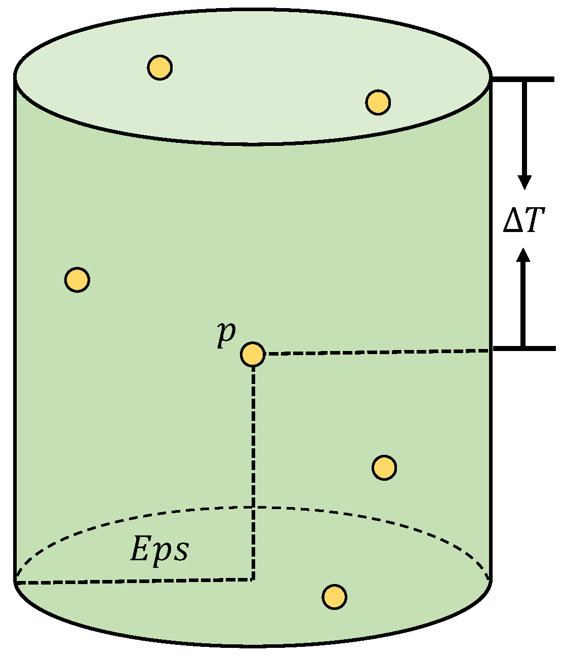
The ST-DBSCAN algorithm adds time dimension on the basis of the DBSCAN algorithm to form a spatial-temporal neighborhood with spatial distance as radius and time interval as height, which is used for the clustering analysis of spatial-temporal data. As shown in Figure 1, the algorithm identifies the density of samples through three parameters, namely space radius E p s , time window Δ T and density threshold M i n p t s . Based on this, the data meeting the conditions are divided to form the final cluster set.
Where E p s is used to measure the distance between two spatial-temporal data in the spatial dimension and Δ T is used to measure the distance in the time dimension. For example, A ( x 1 , y 1 , z 1 , t 1 ) and B ( x 2 , y 2 , z 2 , t 2 ) represent two spatial-temporal data, where ( x 1 , y 1 , z 1 ) and ( x 2 , y 2 , z 2 )   are spatial attributes and t 1 and t 2 are temporal attributes, then the calculation formulas of E p s and Δ T are as follows:
E p s = ( x 1 x 2 ) 2 + ( y 1 y 2 ) 2 + ( z 1 z 2 ) 2
Δ T = | t 1 t 2 |
The ST-DBSCAN algorithm uses the threshold parameter M i n p t s to represent the minimum number of sample points required for clustering in the spatial-temporal neighborhood, which can be obtained from the total number N of microseism events. The calculation formula is as follows:
M i n p t s = l n N
According to the relevant definitions of the ST-DBSCAN algorithm, the algorithm starts loop judgment after inputting the sample data set. If the number of adjacent points within the space radius E p s and time window Δ T of the core point is not less than M i n p t s , a cluster will be formed. Otherwise, the next point will be judged until all points have completed traversal and judgment. The specific construction steps are described as follows:
(1)
Algorithm inputs: sample data set D , spatial radius parameter E p s , time window parameter Δ T , density threshold M i n p t s .
(2)
Establish a tag list L , which is used to mark whether the sample point has completed the traversal state, and initially set the traversal state L = 0 of all points in D .
(3)
Start traversal, randomly select point d in D , and set its traversal state to L = 1 .
(4)
Start loop 1, if the number of points in the E p s and Δ T spatial-temporal neighborhood of d is not less than M i n p t s , create a new cluster C , add d to C , otherwise mark d as a noise point.
(5)
D * represents the set of all points in the E p s and Δ T spatial-temporal neighborhood of d .
(6)
Start loop 2, traversing each point d * in D * .
(7)
If L = 0 of d * , select this point and set L = 1 of d * .
(8)
If the number of points in the E p s and Δ T spatial-temporal neighborhood of d * is not less than M i n p t s , add these points to the set D * .
(9)
If d * does not belong to any cluster, add d * to cluster C .
(10)
End loop 2, and the algorithm outputs the set of cluster C .
(11)
End loop 1, the termination condition of the algorithm is that the traversal states of all data points are L = 1 , that is, all data points have been processed, either classified into a cluster or marked as noise points.

2.2. Support Vector Regression

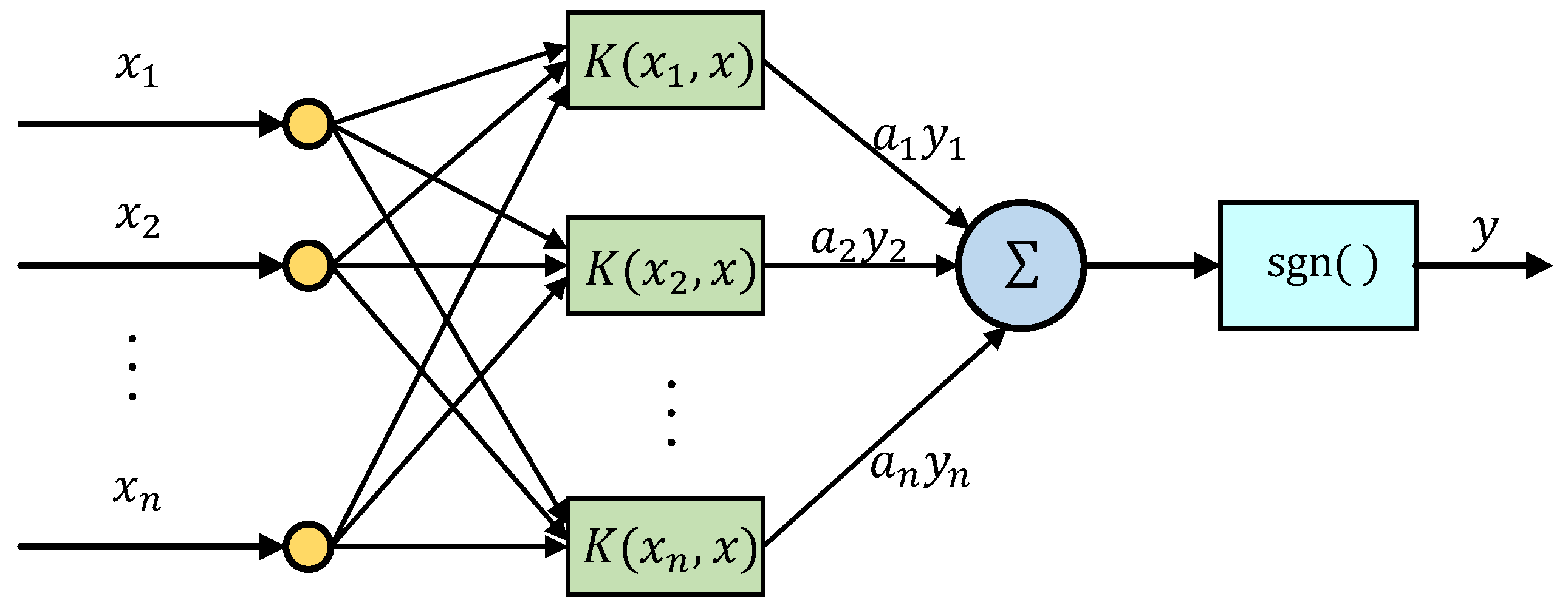
In recent years, the support vector machine (SVM) has been a hot research topic in the field of machine learning applications. It is a machine learning method based on statistical learning theory and the structural risk minimization principle. Because of its good learning ability, the SVM is widely used in many fields of life and production [27,28], mainly to solve the problems of classification and regression analysis. The SVM has a solid mathematical theoretical foundation and excellent performance, so can well solve many key problems of modeling based on neural network, especially the problem of neural network training. The SVM structure is shown in Figure 2:
The traditional SVM is a generalized linear classifier, which is used to solve data classification problem. However, the theory of the SVM can be adjusted so that it can also be applied to regression analysis problem. This improved method is called Support Vector Regression (SVR). It is flexibly applied to the modeling of nonlinear regression problem and can show unique advantage when processing multidimensional or high-dimensional data, because the nonlinear kernel function in the algorithm can map the sample data to a higher dimensional feature space and can quickly find the linear regression function. The SVR algorithm has many advantages, such as low generalization error rate, low computational complexity, not falling into local optimization, and high accuracy in dealing with nonlinear prediction and regression problem. As shown in Figure 3, the objective of the algorithm is to find the function f ( x ) , which wants to maximize the “soft edge ε ” to include as many target values as possible while maintaining a certain flatness.
The regression prediction of data can be realized by finding the decision boundary that maximizes the edge. The function can be expressed as follows:
f ( x ) = ω T x + b
where ω is the weighting coefficient, b is the threshold, also known as the bias term, flatness means that we need to find a ω as small as possible (in the sense of Euclidean norm, that is | | ω | | 2 ). This problem can be transformed into a convex optimization problem:
m i n 1 2 ω 2
s u b j e c t   t o   { y i ω x i b ε ω x i + b y i ε
where ε is the allowable error value of the regression function, and the smaller ε is, the smaller the error of the regression function will be, indicating that the sample points are more concentrated. However, not every sample point in the training set can meet the constraint conditions. Therefore, relaxation variables ξ i + and ξ i can be introduced to alleviate the optimization constraint problem. The above formula can be rewritten as follows:
m i n   L ( ω , ξ i + , ξ i ) = m i n ( 1 2 ω 2 + C i = 1 n ( ξ i + + ξ i ) )
s u b j e c t   t o { y i ω x i b ε + ξ i + ω x i + b y i ε + ξ i ξ i + , ξ i 0
where C is the penalty factor, which is a positive value, indicating the penalty degree of the samples exceeding the allowable error, and is used to adjust the trade-off between the relaxation variable and the boundary. Lagrange multiplier method and duality theory are applied to the above formula, and Lagrange multipliers α + and α are introduced. The objective function can be changed as:
M a x i = 1 l [ y i ( α i + α i ) ε ( α i + + α i ) ] 1 2 i , j = 1 l ( α i + α i ) ( α j + α j ) k ( x i , x j )
s u b j e c t   t o { i = 1 l ( α i + α i ) = 0 0 α i + , α i c
where k ( x i , x j ) is the kernel function, so the final fitting function can be expressed as:
f ( x ) = i , j = 1 l ( α i + α i ) k ( x i , x j ) + b
Common kernel functions include linear kernel, polynomial kernel, sigmoid kernel, and Radial Basis Function (RBF) kernel function. Among them, RBF is the most commonly used kernel function in the SVR algorithm, because it can map sample data to high-dimensional space nonlinearly, and can handle the situation that there is a nonlinear relationship between class labels and sample attributes.

2.3. Long Short-Term Memory

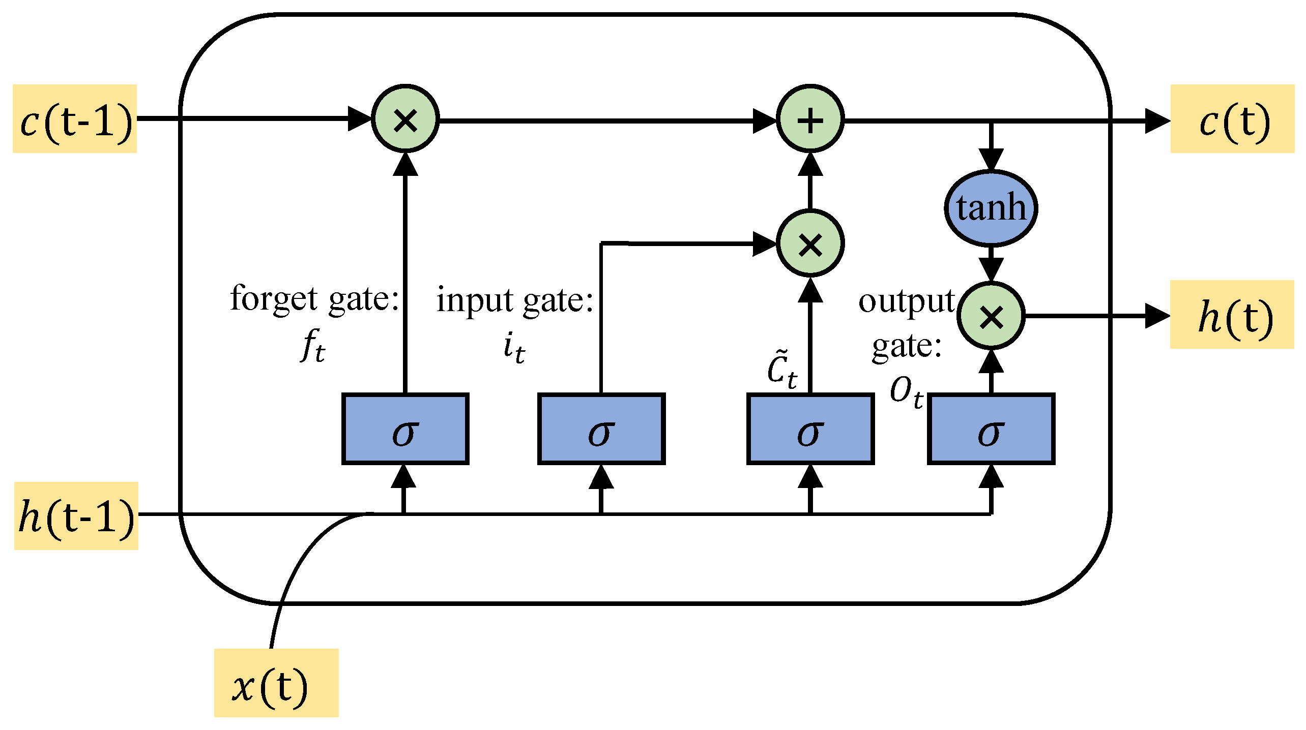
In the Recurrent Neural Network (RNN), information is allowed to be transmitted in different time steps, which is conducive to learning order dependency in input data, making it more suitable for long-time series. Gradient descent is often used in the training of neural networks. However, with the increase of time step, the RNN suffers more and more from gradient disappearance and explosion, which aggravates the difficulty of model training. In order to solve this problem, the LSTM is developed based on the RNN model. The LSTM model structure is shown in Figure 4, including a core unit (memory part) and three gating structures (forget, input and output gates), which guide the information flow inside the LSTM unit.
The calculation steps of LSTM are as follows:
(1)
Determine the information to discard in the cell state. Input the output h t 1 at the last moment and the input x t at the current moment, through the forget gate, add the Sigmoid function, and output a vector whose element values are between 0 and 1, which represents the stored proportion of the cell state C t 1 at the last moment. The calculation formula is:
f t = σ ( W f [ h t 1 , x t ] + b f )
(2)
Determine the new information stored in the cell state. There are two steps: the input gate determines the updated value, and the candidate value vector i t is then added to the cell state. The calculation formula of the input gate value and the new candidate value vector C ˜ t are as follows:
i t = σ ( W i [ h t 1 , x t ] + b i )
C ˜ t = t a n h ( W C [ h t 1 , x t ] + b C )
(3)
Update the states of old cells. C t 1 is updated to C t by discarding some of the information and adding new candidate values. The calculation formula of cell state value at the current moment is:
C t = f t C t 1 + i t C ˜ t
(4)
Determine the value of the output. It includes two steps: determine the value O t of the output gate, and then determine the final output result value h t at the current moment. The calculation formula is as follows:
O t = σ ( W o [ h t 1 , x t ] + b o )
h t = O t tan h ( C t )
where W f , W i , W C and W o are the weight terms to be learned, b f ,   b i , b C and b o are the offset terms to be learned, σ is the Sigmoid activation function,   is the Hadamard product, where the components of vectors are multiplied one by one. The key advantage of using the LSTM unit is that the cell state will be updated dynamically with the passage of time, which increases the processable sequence length of time-series neural network and has better effect on prediction tasks with long-term regularity.

3. Model Design

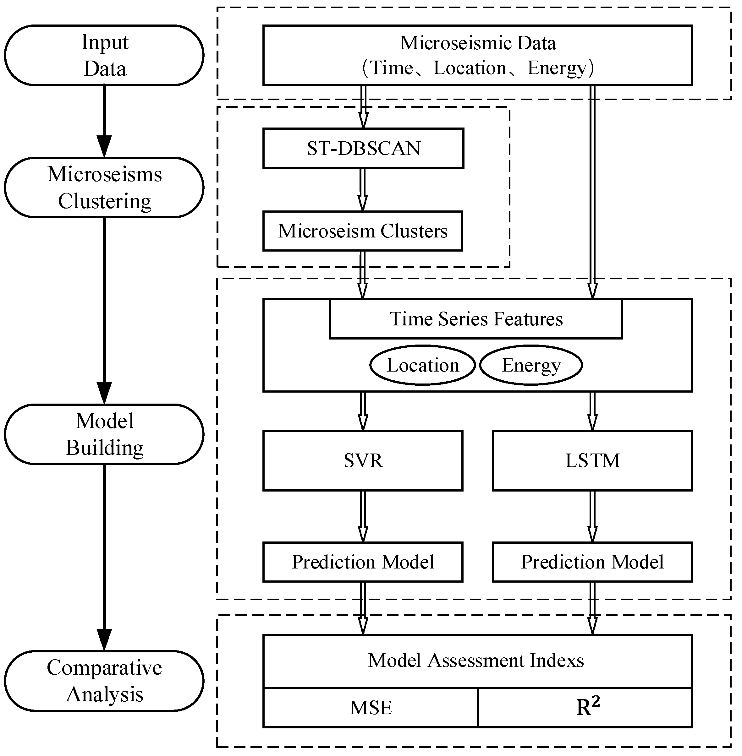
With regard to the prediction and early warning of high-energy mine earthquake, it is difficult for the traditional experience-driven and mechanism-driven strategies to accurately answer the three key questions of when, where, and energy level [29]. This gives machine learning a chance. In fact, the data-driven method has a better solution to those questions. At present, most research follows a fixed model, that is, select a machine learning model and find the best results through parameter optimization. However, if the microseism data are directly input into the training model, the final prediction accuracy is often not high, because the microseisms are not isolated events, but have obvious spatial-temporal aggregation. Therefore, if the spatial-temporal clustering analysis of microseism events is carried out first, the closely related microseism events will be divided into clusters, so the correlation degree between microseism data will be improved. On this basis, the machine learning method is used to fit this rule and establish a prediction model, which can significantly improve the accuracy of mine earthquake prediction. Accordingly, we propose a time sequence prediction method for mine earthquake combined with clustering analysis. The specific process is shown in Figure 5, which mainly includes three parts.
(1)
The clustering of microseism events. Similar to earthquake, coal mine microseisms are in essence a kind of dynamic phenomenon caused by stress release. Generally, they do not appear as isolated events, but many microseism events with different energy levels will occur successively in a certain region and time period, to form swarm sequences. The microseism events included in a swarm sequence are caused by a stress release, so the occurrence time, location, and energy levels of these microseism events have a certain regularity. In the ST-DBSCAN algorithm, the density is obtained by calculating the number of adjacent points in the designated spatial-temporal neighborhood around the sample point. The points whose density are higher than the designated threshold will be constructed as clusters, which are very suitable for processing the spatial-temporal data recorded in the microseism monitoring system. Clustering analysis can identify the active areas of microseism events in the working face and divide the microseism events into closely related clusters. The time, location, and energy information of microseism events contained in each cluster can be regarded as time series data [30] and have a certain regularity.
(2)
The establishment of a prediction model. After the completion of cluster analysis, microseism events on the working face will be divided into clusters. Although the correlation degree between microseism events in the cluster increases, the number of microseism events in a cluster is not large. This is equivalent to dividing a large sample data set containing microseism events of the whole working face into many small sample data sets. Therefore, the SVR algorithm suitable for small samples is selected to predict the time series of microseism events within the cluster. Mine earthquake prediction includes two aspects: one is the location of high-energy events; the second is the daily frequency of high-energy events with different energy levels, that is, the information of microseism events that have occurred in a specific period of time is used to predict the possible occurrence location (X, Y and Z coordinates) and the daily frequency of subsequent high-energy events.
(3)
The comparative analysis of the model. In order to verify the effectiveness of the proposed method which uses SVR to predict mine earthquake on the basis of clustering analysis, the LSTM, a very classical method in time sequence prediction, is selected for comparison experiment. Similarly, the occurrence location (X, Y and Z coordinates) and the daily frequency of high-energy events are predicted. At the same time, the effects of the two prediction models are compared and evaluated by using the Mean Square Error (MSE) and R-square (R2). The data used by the LSTM here is the microseism data of the whole working face, without clustering analysis. On the one hand, it is to compare the effect of clustering analysis on improving the accuracy of machine learning prediction model, and on the other hand, it also meets the requirement of method for large sample size.
The proposed framework consists of the ST-DBSCAN and SVR algorithms, so its time complexity depends on the time complexity of the two algorithms. When the ST-DBSCAN runs, it needs to traverse all the points in the dataset and calculate the number of density-reachable points of each point, so its time complexity is O ( N 2 ) , where N is the number of the training samples. Meanwhile, the time complexity of SVR is O ( N 3 ) [31]. Only the item with the fastest growth rate is considered, so the time complexity of proposed framework is O ( N 3 ) .

4. Engineering Experiments

4.1. Microseism Data Acquisition

The data in this paper comes from the real-time microseism data collected by the SOS microseism monitoring system from Poland, specifically the microseism data of 103# working face of the H Coal Mine, with a total of 8497 records. As shown in Table 1, each record contains the time, location, and energy information of microseism.
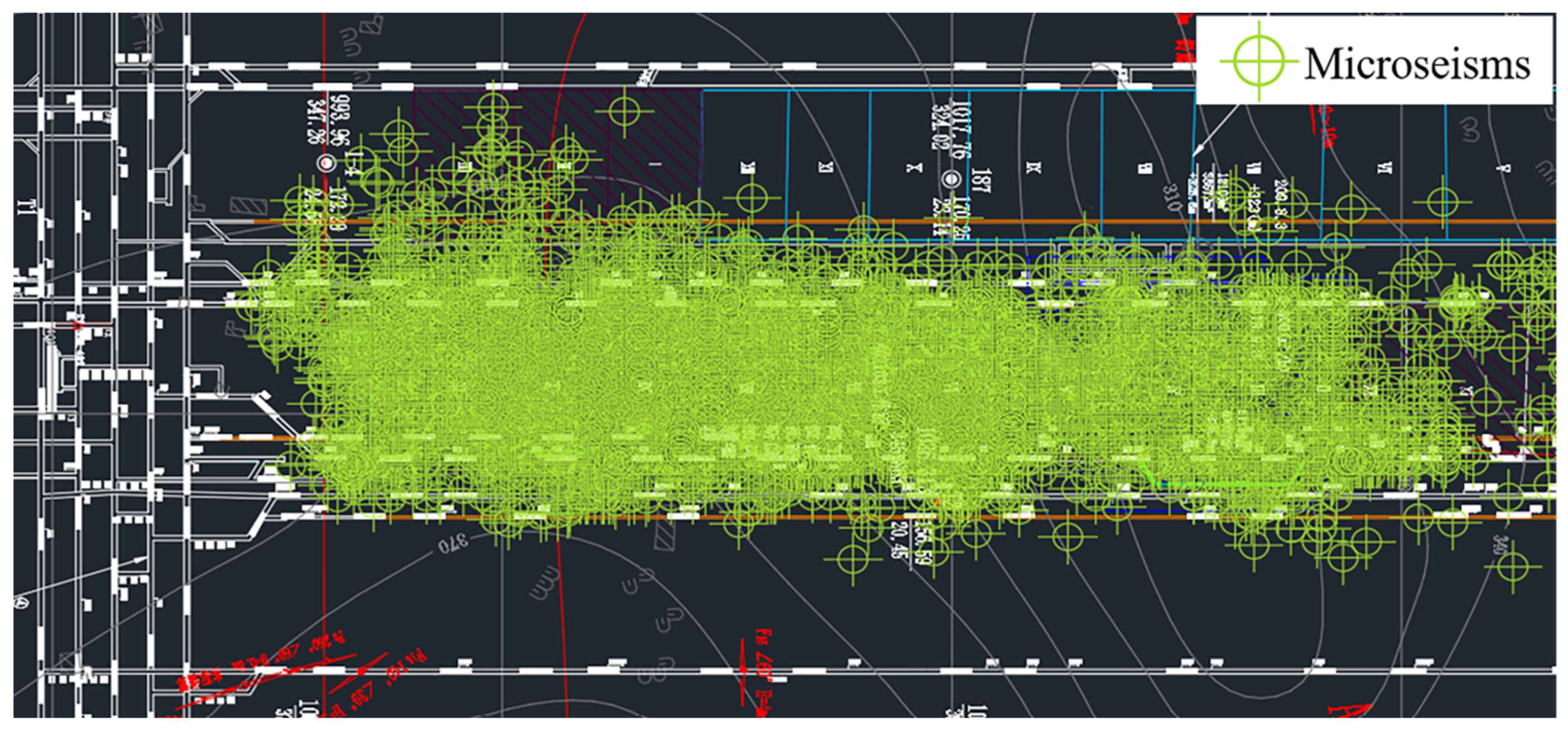
These microseism events are presented in the mining engineering plan, as shown in Figure 6. It can be seen that microseism events cover the whole target working face.
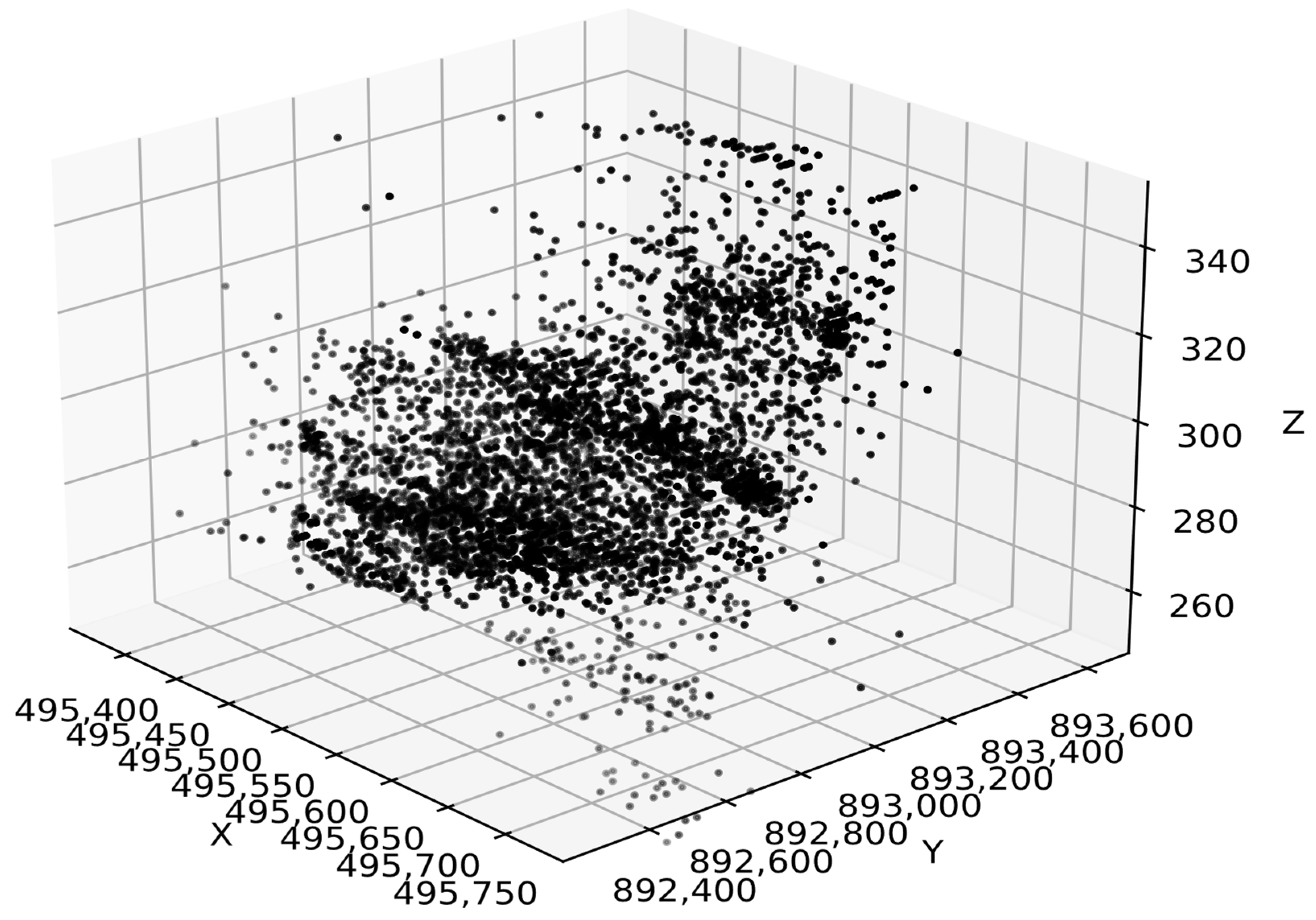
The distribution of microseisms in three-dimensional space is shown in Figure 7.

4.2. Clustering of Microseism Events

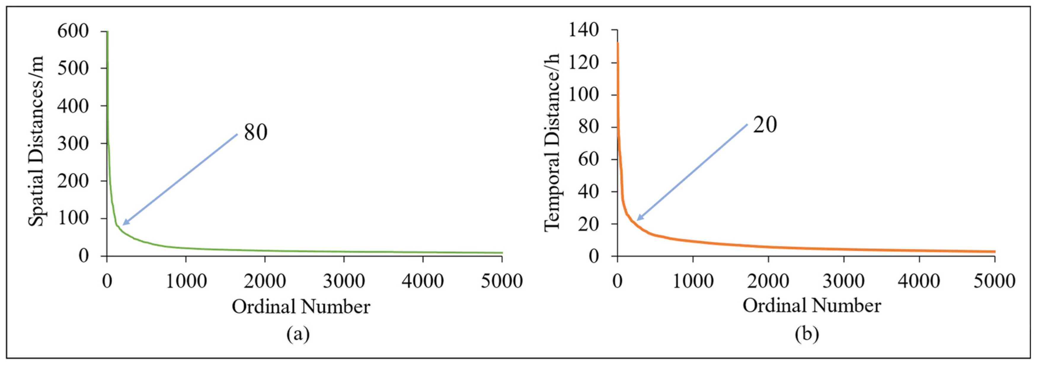
The ST-DBSCAN algorithm is used to cluster microseism events in the target working face. According to the empirical formula (3), M i n p t s = l n N 9   can be calculated. The spatial radius E p s and time window   Δ T   of the cluster are obtained from the K-Dist graph [32], where K takes the value of M i n p t s , which is 9 at this time. The specific steps are to calculate the spatial distance and temporal distance between each sample point and the ninth closest point, and draw the corresponding 9-Dist graph in descending order, the distance value corresponding to the inflection point is the effective radius of dividing the noise point and the non-noise point. The 9-Dist graph is shown in the following Figure 8.
By observing Figure 8, the vertical axis coordinate values corresponding to the two inflection points are 80 and 20, respectively. However, considering the influence of human factors, there may be subjective errors in the vertical axis coordinate values. In order to find the parameters with the best clustering results, different distance values corresponding to inflection points were selected to carry out the parameter combination clustering tests. E p s   was taken as [70 80 90], and   Δ T   was taken as [15 20 25]. In Table 2, nine parameter combinations can be obtained based on the different values of E p s and Δ T , numbered ID1 to ID9. respectively.
In order to measure the effect of clustering, the Silhouette Coefficient (SC) is selected as the clustering effectiveness assessment index [33]. Generally speaking, the higher the average SC of the samples in the clusters, the better the clustering quality. For any point i in the cluster, the SC is calculated as follows:
S C ( i ) = b ( i ) a ( i ) max { a ( i ) , b ( i ) }  
where a ( i ) is the degree of dissimilarity within the cluster, representing the average value of the degree of dissimilarity from point i to other points in the same cluster, reflecting the degree of cohesion; b ( i ) is the degree of dissimilarity between clusters, representing the minimum value of the average degree of dissimilarity from point i to other clusters, reflecting the degree of separation. It can be seen that the value of SC is between [−1, 1], and the closer it is to 1, the better cohesion and separation degree are. The average of the SC of all points is the comprehensive SC of the clustering result.
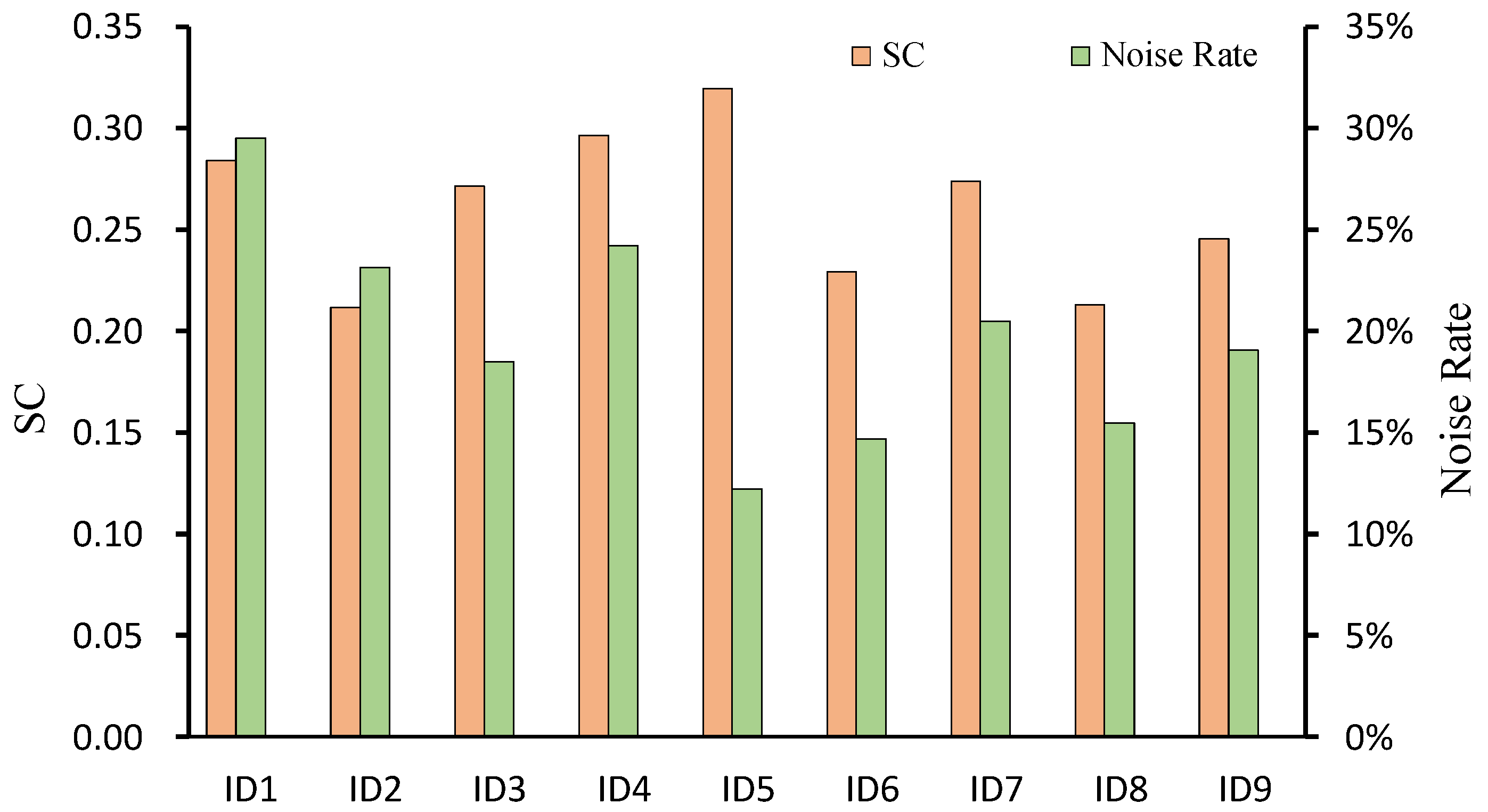
The clustering algorithm program is run on the nine parameter combinations in Table 2, and the output results are the specific cluster sets and noise points that are not classified into any clusters. Different parameter combinations of E p s and Δ T will get different clustering results. Their SC are calculated respectively and the noise rate is counted. The results are shown in Table 3 and Figure 9.
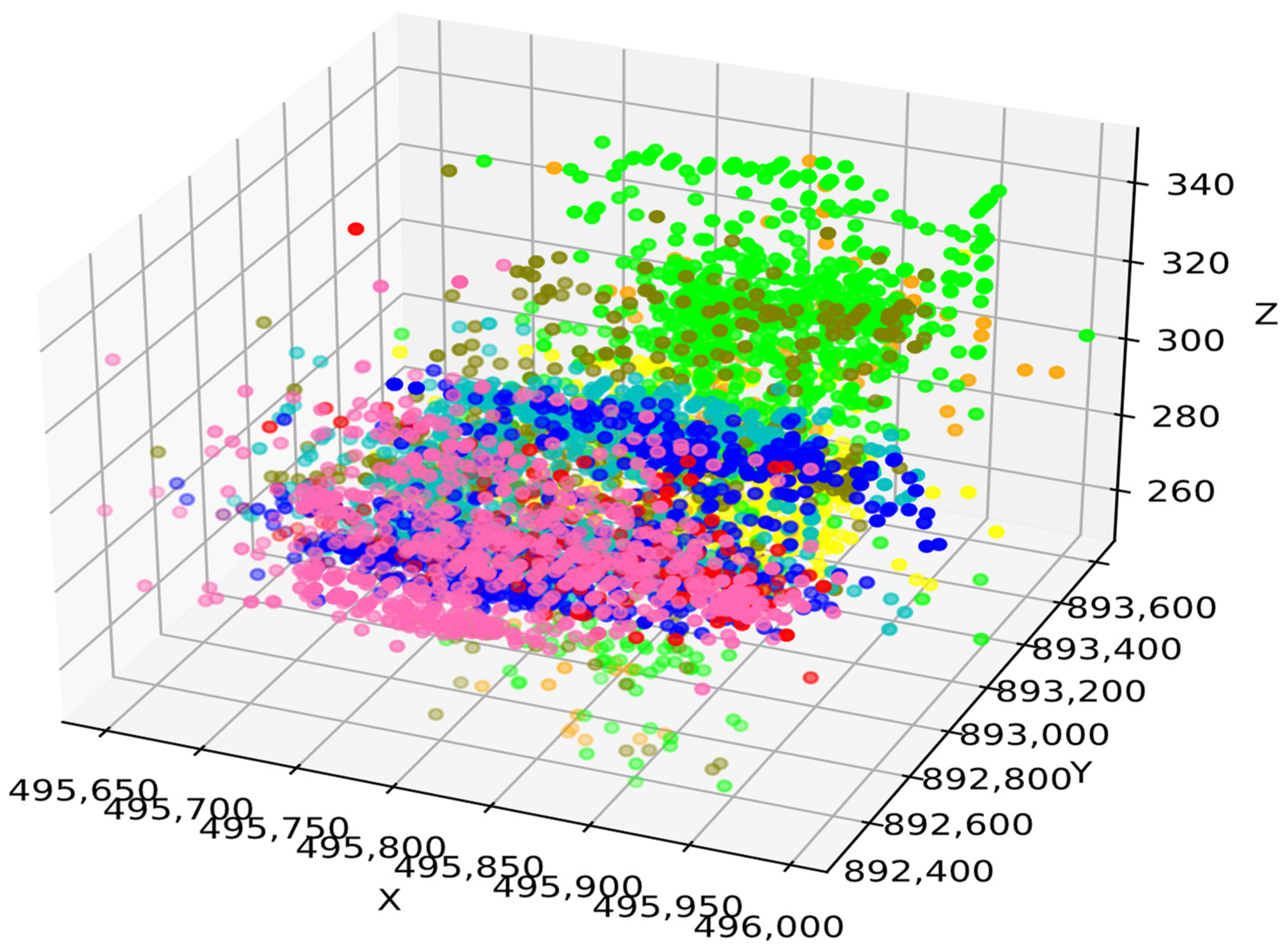
It can be easily seen from Figure 9 that the SC of ID5 is high and the noise rate is low. Therefore, when E p s is set to 80 and Δ T is set to 20, the clustering result is the best. Different colors are used to represent different clusters, and the clustering result of this parameter combination is presented in three-dimensional space, as shown in Figure 10.
At this time, the noise rate is 12.2%, and 47 microseism clusters are obtained, and the largest cluster contains 1077 events. Due to space limitation, some statistical results are shown in Table 4.
Several clusters containing more microseism events are projected into the mining engineering plan. The results are shown in Figure 11. Compared with Figure 6, it can be seen that microseism events have obvious aggregation. Clustering analysis of microseism events can be regarded as a preprocessing process for subsequent prediction data. The purpose is to remove interference factors, enhance the correlation between sample data and improve the accuracy of prediction models.

4.3. Prediction of Mine Earthquake

The microseism clusters can be regarded as mine earthquake sequences. The location and frequency corresponding to different energy levels of events in the cluster have a time-series law, that is, the location and frequency of subsequent microseism events are related to historical microseism information. The largest microseism cluster containing 1077 events was selected, and the SVR was used to establish a model to conduct prediction experiment in sequence for the microseism events in the cluster. The prediction includes two aspects: occurrence location, and daily frequency of high-energy event. Generally, when the energy released by mine earthquake reaches above 10 4   J , the rock burst may be induced, causing serious injury to underground roadway and personnel [34]. Therefore, the high-energy event refers to the mine earthquake event that releases energy greater than 10 4   J . In data preprocessing, considering the strong correlation of microseism events within the cluster and the limited number of events, the sampling step of position prediction is 10 times, the sampling step of frequency prediction is 3 days, and the moving step is 1. In order to evaluate the prediction effect of model, MSE and R2 are selected as assessment indexes [35], and their calculation formulas are as follows:
M S E = 1 n   n i = 1 ( y i y ^ i ) 2
R 2 = 1 i = 1 n ( y i y ^ i ) 2 i = 1 n ( y i y ¯ ) 2  
where n is the total number of samples, y ^ i is the predicted value, y i is the true value of the sample, y ¯ is the mean of the true value. The smaller the value of MSE is, the more accurate the model prediction is. R2 is between (−∞, 1], and the larger the value is, the better the effect of model fitting ability is.

4.3.1. Prediction for Location of High-Energy Events

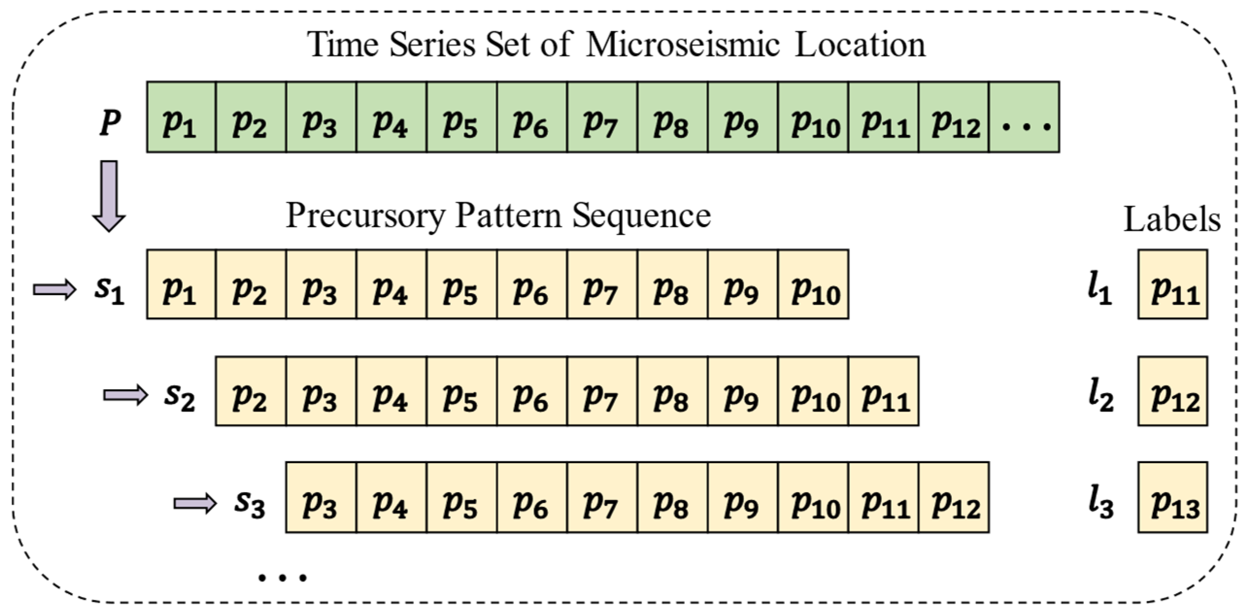
It is of great significance to predict the location of high-energy mine earthquake for the prevention and control of underground dynamic disasters in coal mines. The specific method is extracting the high-energy events with release energy greater than 10 4   J from the cluster, using the related information of the previous 10 mine earthquakes to predict the location of the next event. The precursory pattern sequence features of the model include the X, Y, Z coordinate values and the distance between two events immediately adjacent to each other of the previous 10 events. The corresponding label is the location of the next event, that is, the X, Y, Z coordinate values. As shown in Figure 12 below, P = ( p 1 , p 2 , p 3 , , p n )   is the time series set of microseism location information, where p i is the location information of one event. When the sampling step is 10 and the moving step is 1, the precursory pattern sequence set S = ( s 1 , s 2 , s 3 , , s u ) can be obtained, where s i is a precursory pattern sequence, which contains the location information of the previous ten microseism events. The label set corresponding to S is L = ( l 1 , l 2 , l 3 , , l u ) ,where l i is the label corresponding to s i and contains the location coordinates of the next microseism event.
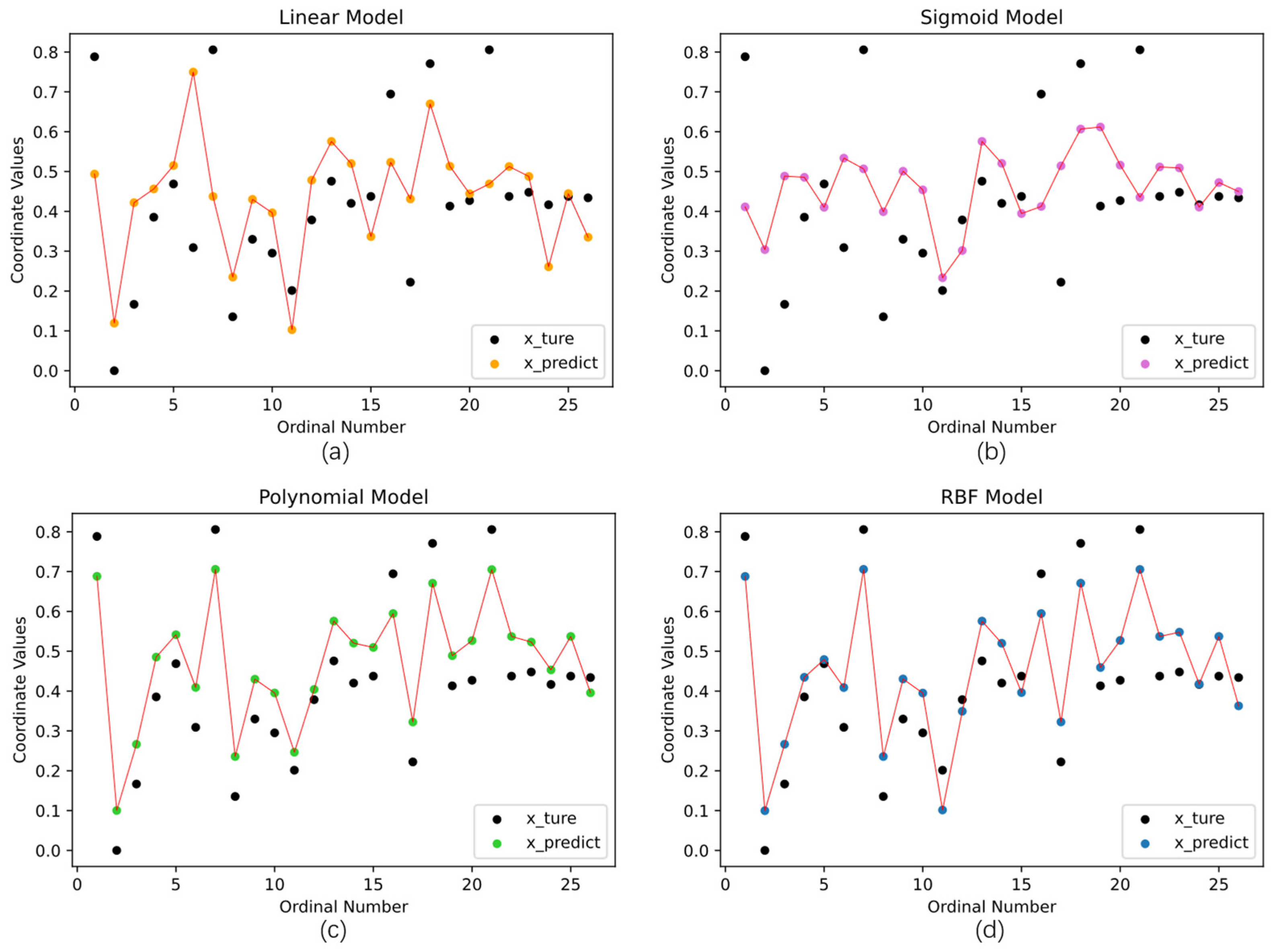
The statistical result was n = 97. After P was processed as shown in the Figure 12, u = 87 was obtained, that is, the prediction model would have 87 samples and corresponding labels. The samples were divided into training set and test set according to the ratio of 7:3. The training set was used for the simulation training of the model, and the test set was used to test the effect of the training. Four kernel functions of SVR, Linear, Sigmoid, Polynomial and RBF, were selected for the experiment, and the grid search method was used to optimize the hyperparameters of model. Overfitting can be suppressed by two parameters. One is the penalty factor C, the higher its value is, the more intolerant the model is to errors and easy to overfit. The other is the parameter gamma in the kernel function. With the increase of gamma, the prediction effect of the training set becomes better, and the prediction effect of the test set becomes worse. At the same time, the complexity of the model increases, and the generalization ability becomes worse, which leads to the overfitting. The overfitting issue is controlled by adjusting the above two parameters combined with the final prediction effect of the model.
The predicted values outputted from model and the true values were compared together to get Figure 13 below. In view of the equal position of X, Y and Z coordinates in location prediction, this case only presents the prediction of X coordinates due to space limitation. The MSE and R2 of the four prediction models with different kernel functions in the figure were calculated respectively, and the statistical results are shown in Table 5.
Combined with Figure 13 and Table 5, it can be seen that the SVR model with RBF kernel function has the best effect on the location prediction of high-energy mine earthquakes.

4.3.2. Prediction for Frequency of High-Energy Events

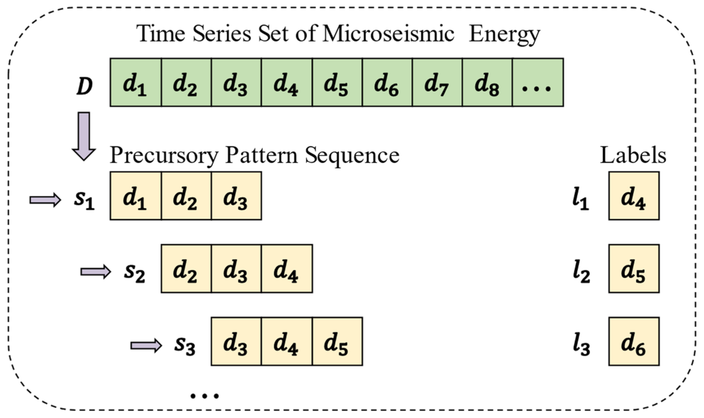
For the microseism events in the cluster, the occurrence frequencies corresponding to different energy levels are counted every day. The energy levels are divided according to 10 2   J , 10 3   J , 10 4   J , 10 5   J ... As with the location prediction, only high-energy events with energy above 10 4   J are selected as the prediction objects. The specific method is using the related frequency information of the previous three days, to predict the occurrence frequency of high-energy events in the next day. Therefore, the precursory pattern sequence features of the model are the daily occurrence frequency of microseism events with different energy levels in the previous three days, and the corresponding label is the occurrence frequency of high-energy mine earthquakes with different energy level in the next day. As shown in Figure 14, D = ( d 1 , d 2 , d 3 , , d m ) is the time series set of microseism energy information, where d i is the energy frequency data within a day. When the sampling step is 3 and the moving step is 1, the precursory pattern sequence set S = ( s 1 , s 2 , s 3 , , s v ) can be obtained, where s i is a precursory pattern sequence, which contains the energy frequency information of the previous three days. The corresponding label set is L = ( l 1 , l 2 , l 3 , , l v ) , where l i is the label corresponding to s i and contains the occurrence frequency of mine earthquakes with energy level above 10 4 J in the following day.
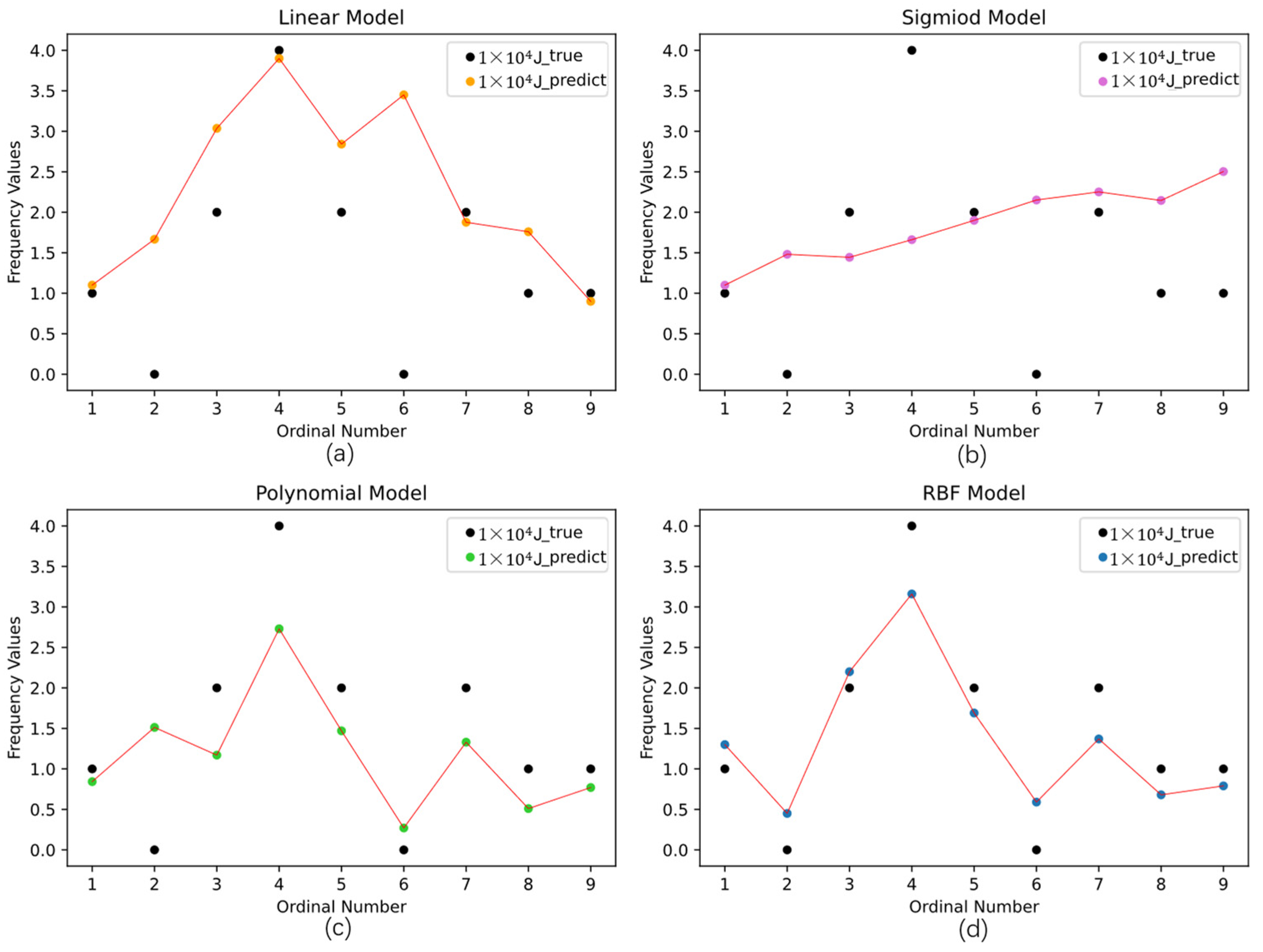
The statistical result was m = 31. After D was processed as shown in the Figure 14, v = 28 was obtained, that is, the prediction model would have 28 samples and corresponding labels. The samples were divided into training set and test set according to the ratio of 7:3. The training set was used for the simulation training of the model, and the test set was used to test the effect of the training. Four kernel functions of SVR, Linear, Sigmoid, Polynomial and RBF, were selected for the experiment, and the grid search method was used to optimize the hyperparameters of model. The predicted values outputted from model and the true values were compared together to get Figure 15. In view of the equal position of different energy levels in energy frequency prediction, this case only presents the prediction of daily frequency of 10 4   J level mine earthquake due to space limitation. The MSE and R2 of the four prediction models with different kernel functions in the figure were calculated respectively, and the statistical results are shown in Table 6.
Combined with Figure 15 and Table 6, it can be seen that the SVR model with RBF kernel function has the best prediction effect on the daily frequency of high-energy mine earthquakes with different energy levels.

4.4. Comparison of Prediction Models

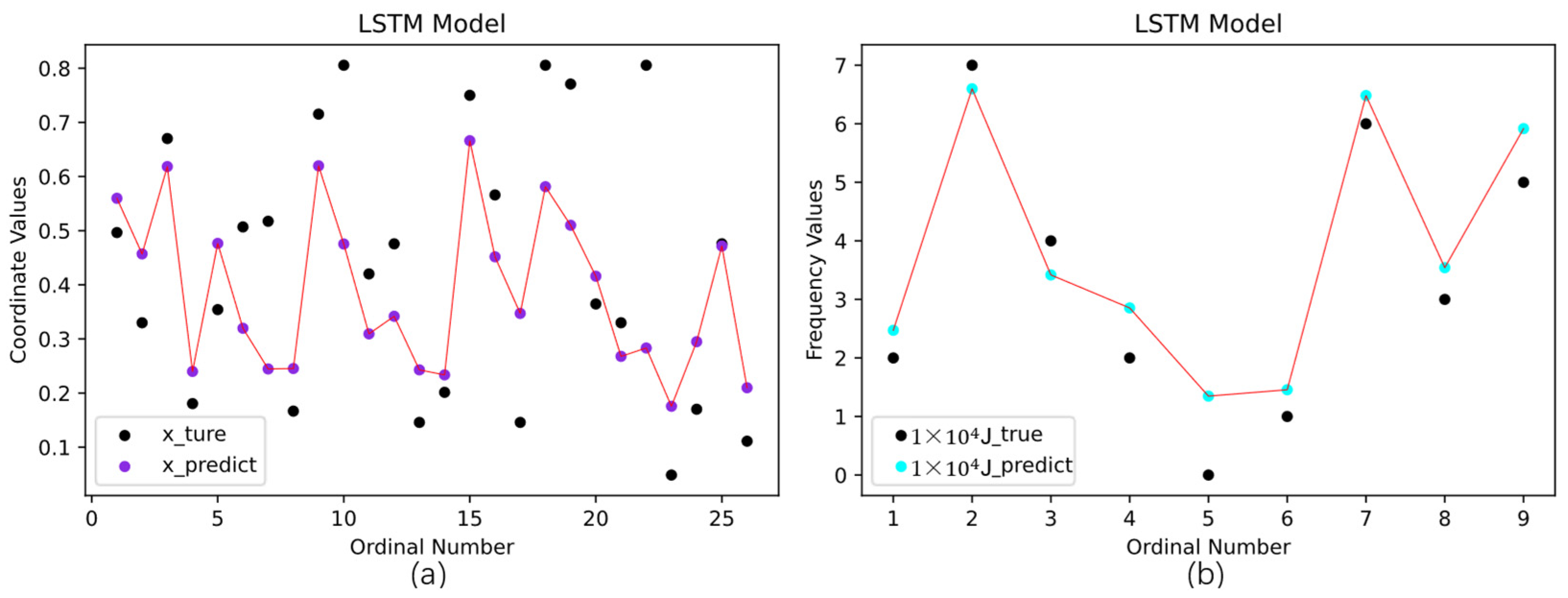
As a comparison experiment, the LSTM was used to build a prediction model, and the model was trained on the microseism dataset (including 8497 event records) of 103# working face without clustering process, and used to predict the location of high-energy mine earthquakes and the daily occurrence frequency corresponding to different energy levels. In the SVR model above, the microseism data used was distributed from April 23 to May 23, so the event samples in the test set of the LSTM prediction model were also set within this time period. The time series sets of microseism location information and energy frequency information were also processed respectively as shown in Figure 12 and Figure 14 to obtain n = 1320, u = 1310, m = 562, v = 559. The Early Stopping method was used to prevent the overfitting issue. The specific method is to calculate the accuracy of validation data at the end of each epoch training. When the accuracy does not improve any more, the model training will be stopped to avoid overfitting. Similarly, the grid search method was used to optimize the hyperparameters of model, and the prediction of X coordinates of high-energy mine earthquakes and daily occurrence frequency corresponding to 10 4   J energy level events are shown in Figure 16:
In the SVR model, the RBF kernel function has the best prediction effect. Therefore, the MSE and R2 of the LSTM model in predicting the X coordinates of high-energy events and the daily frequency corresponding to 10 4   J energy level events are calculated and compared with the former. The results are shown in Table 7.
Through comparative experiments, it can be concluded that the SVR model with RBF kernel function on the basis of clustering analysis is better than the LSTM model without clustering analysis, both for the prediction of the location of high-energy mine earthquakes and the prediction of daily frequency of high-energy mine earthquakes with different energy levels.

4.5. Out-of-Sample Prediction Experiment

Save the trained model and feed it the microseism data of a new cluster, which was not involved in the previous model training process. The final performance is shown in Table 8. It can be seen that the prediction effect of the trained SVR model with RBF kernel on the new cluster is not as good as that of the LSTM model using global data. This indicates that the time series laws of data in different clusters may not be the same, due to the influence of the changing geological conditions and other factors, and the trained SVR model cannot be simply and directly applied to the new cluster. Its parameters need to be adjusted to get a good performance on different clusters.

5. Conclusions

It is easy for mine earthquake activity to cause coal mine dynamic disasters, resulting in serious consequences. The microseism monitoring system can monitor the microseism events in real-time and record the time, space, and intensity information when the mine earthquake occurs. In this paper, the microseism data of 103# working face of the H Coal Mine were selected. Firstly, the ST-DBSCAN algorithm was used to find out the microseism clusters, and then SVR was used to predict the occurrence location and daily frequency of high-energy events on this basis. MSE and R2 were selected as the assessment indexes of the model prediction effect. The results (Table 5 and Table 6) showed that among the four different kernel functions, the SVR prediction model with RBF kernel function has the best performance. Finally, as a comparison experiment, the LSTM model was used to predict high-energy mine earthquakes in the same period using the 103# working face microseism data without clustering process. Through comparative analysis, its performance (Table 7) was inferior to the SVR prediction model with RBF kernel function. This engineering experiment showed that the spatial-temporal clustering analysis of microseism events in advance can improve the prediction accuracy of the machine learning method on high-energy mine earthquakes.
However, results of out-of-sample prediction experiment (Table 8) showed that the trained SVR model does not perform well on the new cluster. The reason could be that the time series laws of data in different clusters are not exactly the same, due to the influence of the changing geological conditions and other factors. In future work, we will conduct research on the model’s generalization ability on different microseism events clusters and mines.

Author Contributions

Conceptualization, X.L. and P.Z.; methodology, P.Z. and J.C. All authors have read and agreed to the published version of the manuscript.

Funding

This research was funded by National Key Research and Development Program of China (Grant no.2020YFB1314200) and China Postdoctoral Science Foundation (Grant no.2018M642367).

Institutional Review Board Statement

Not applicable.

Informed Consent Statement

Not applicable.

Data Availability Statement

Not applicable.

Acknowledgments

The authors would like to thank the anonymous referees for their valuable comments and suggestions.

Conflicts of Interest

The authors declare no conflict of interest.

References

  1. Zhang, S.; Guan, J.; Liu, L.; Teng, X. Progress in research on mine earthquakes. Recent Dev. World Seismol. 1994, 52, 1–6. [Google Scholar]
  2. Cao, A.; Chen, F.; Liu, Y.; Dou, L.; Wang, C. Response characteristics of rupture mechanism and source parameters of mining tremors in frequent coal burst area. J. China Coal Soc. 2022, 47, 722–733. [Google Scholar]
  3. Qi, Q.; Dou, L. Rock Burst Theory and Technology, 1st ed.; China University of Mining and Technology Press: Xuzhou, China, 2008. [Google Scholar]
  4. Dou, L.; Cao, J.; Cao, A.; Cai, Y.; Bai, J.; Kan, J. Research on types of coal mine tremor and propagation law of shock waves. Coal Sci. Technol. 2021, 49, 23–31. [Google Scholar]
  5. Alber, M.; Fritschen, R.; Bischoff, M.; Meier, T. Rock mechanical investigations of seismic events in a deep longwall coal mine-ScienceDirect. Int. J. Rock Mech. Min. Sci. 2009, 46, 408–420. [Google Scholar] [CrossRef]
  6. Zheng, C. Study on Characterization Method of Rock Mass Strength Parameters in Mines Based on Microseism Monitoring Data. Ph.D. Thesis, Northeastern University, Shenyang, China, 2013. [Google Scholar]
  7. Gong, S.; Dou, L.; Cao, A.; He, H.; Du, T.; Jiang, H. Study on optimal configuration of seismological observation network for coal mine. Chin. J. Geophys. 2010, 53, 457–465. [Google Scholar]
  8. He, H.; Dou, L.; Gong, S.; Zhou, P.; Xue, Z. Rock burst rules induced by cracking of overlying key stratum. Chin. J. Geotech. Eng. 2010, 32, 1260–1265. [Google Scholar]
  9. Yuan, R.; Li, H.; Li, H. Distribution of microseism signal and discrimination of portentous information of pillar type rockburst. Chin. J. Rock Mech. Eng. 2012, 31, 80–85. [Google Scholar]
  10. Wang, S. Power spectrum laws of microseism signal before and after rock burst. Saf. Coal Mines 2013, 44, 50–52. [Google Scholar]
  11. Xiao, Y.; Feng, X.; Chen, B.; Feng, G. Evolution of frequency spectrum during instant rockbursts in deep inoculation tunnel. Rock Soil Mech. 2015, 36, 1127–1134. [Google Scholar]
  12. Wei, S.; Yang, Y. Spectrum characteristic analysis of rock burst microseism signal in Yimei Mining Area. Saf. Coal Mines 2015, 46, 181–184+188. [Google Scholar]
  13. Peng, M. Category of microseism signals and time-space analysis of microseism event in Liyazhuang Coal Mine. Min. Saf. Environ. Prot. 2019, 46, 87–91. [Google Scholar]
  14. Vallejos, J.A.; Mckinnon, S.D. Logistic regression and neural network classification of seismic records. Int. J. Rock Mech. Min. Sci. 2013, 62, 86–95. [Google Scholar] [CrossRef]
  15. Dong, L.; Wesseloo, J.; Potvin, Y.; Li, X. Discrimination of mine seismic events and blasts using the Fisher classifier, Naive Bayesian classifier and Logistic Regression. Rock Mech. Rock Eng. 2016, 49, 183–211. [Google Scholar] [CrossRef]
  16. Pezzo, E.D.; Esposito, A.; Giudicepietro, F.; Marinaro, M.; Martin, M.; Scarpetta, S. Discrimination of earthquakes and underwater explosions using neural networks. Bull. Seismol. Soc. Am. 2003, 93, 215–223. [Google Scholar] [CrossRef]
  17. Dong, L.; Li, X.; Peng, K. Prediction of rockburst classification using Random Forest. Trans. Nonferrous Met. Soc. China 2013, 23, 472–477. [Google Scholar] [CrossRef]
  18. Ng, A.Y.; Jordan, M.I. On discriminative vs. generative classifiers: A comparison of logistic regression and naive bayes. In Proceedings of the Advances in Neural Information Processing Systems 14, Vancouver, BC, Canada, 3–6 December 2001; pp. 605–610. [Google Scholar]
  19. Dong, L.; Li, X.; Xie, G. Nonlinear methodologies for identifying seismic event and nuclear explosion using Random Forest, Support Vector Machine, and Naive Bayes Classification. Abstr. Appl. Anal. 2014, 2014, 459137. [Google Scholar] [CrossRef] [Green Version]
  20. Ruano, A.E.; Madureira, G.; Barros, O.; Khosravani, H.; Ruano, M.; Ferreira, P. Seismic detection using support vector machines. Neurocomputing 2014, 135, 273–283. [Google Scholar] [CrossRef]
  21. Birant, D.; Kut, A. ST-DBSCAN: An algorithm for clustering spatial–temporal data. Data Knowl. Eng. 2007, 60, 208–221. [Google Scholar] [CrossRef]
  22. Cortes, C.; Vapnik, V. Support-Vector Networks. Mach. Learn. 1995, 20, 273–297. [Google Scholar] [CrossRef]
  23. Vapnik, V. The Nature of Statistical Learning Theory, 2nd ed.; Springer: New York, NY, USA, 2000. [Google Scholar]
  24. Ding, S.; Qi, B.; Tang, H. An overview on theory and algorithm of support vector machines. J. Univ. Electron. Sci. Technol. China 2011, 40, 2–10. [Google Scholar]
  25. Hochreiter, S.; Schmidhuber, J. Long Short-Term Memory. Neural Comput. 1997, 9, 1735–1780. [Google Scholar] [CrossRef] [PubMed]
  26. Zhang, Z.; Liu, H.; Ding, L.; Wu, P.; Yu, G. Identifying moves of research abstracts with deep learning methods. Data Anal. Knowl. Discov. 2019, 3, 1–9. [Google Scholar]
  27. Chen, B.; Fan, X.; Zhou, Z.; Li, X. The principle and prospect of support vector machine. Manuf. Autom. 2010, 32, 136–138. [Google Scholar]
  28. Huang, S.; Cai, N.; Pacheco, P.P.; Narrandes, S.; Wang, Y.; Xu, W. Applications of support vector machine (SVM) learning in cancer genomics. Cancer Genom. Proteom. 2018, 15, 41–51. [Google Scholar]
  29. Chen, J.; Gao, J.; Pu, Y.; Jiang, D.; Qi, Q.; Wen, Z. Machine learning method for predicting and warning of rockbursts. J. Min. Strat. Control. Eng. 2021, 3, 57–68. [Google Scholar]
  30. Raubitzek, S.; Neubauer, T. A fractal interpolation approach to improve neural network predictions for difficult time series data. Expert Syst. Appl. 2021, 169, 114474. [Google Scholar] [CrossRef]
  31. Yu, H.; Sun, W.; Zhou, X.; Zhu, G.; Hu, W. Heuristic sample reduction based support vector regression method. In Proceedings of the 2016 IEEE International Conference on Mechatronics and Automation, Harbin, China, 7–10 August 2016; pp. 2065–2069. [Google Scholar]
  32. Lai, L.; Nie, R.; Wang, J.; Huang, J. Improved DBSCAN algorithm based on mapreduce. Comput. Sci. 2015, 42, 396–399. [Google Scholar]
  33. Yang, H.; Fu, Y.; Fan, D. Influence of noisy features on internal validation of clustering. Comput. Sci. 2018, 45, 22–30+52. [Google Scholar]
  34. Cao, A.; Liu, Y.; Yang, X.; Li, S.; Liu, Y. FDNet: Knowledge and data fusion-driven deep neural network for coal burst prediction. Sensors 2022, 22, 3088. [Google Scholar] [CrossRef]
  35. Yang, Y. Noninvasive Blood Pressure Measurement Based on Deep Learning. Ph.D. Dissertation, Nanjing University of Information Science and Technology, Nanjing, China, 2022. [Google Scholar]
Figure 1. Schematic representation of the spatial-temporal neighborhood.
Applsci 12 11101 g001
Figure 2. Schematic diagram of SVM structure.
Applsci 12 11101 g002
Figure 3. Basic concept diagram of SVR.
Applsci 12 11101 g003
Figure 4. Schematic diagram of LSTM structure.
Applsci 12 11101 g004
Figure 5. The workflow of mine earthquake prediction in time sequence.
Applsci 12 11101 g005
Figure 6. Distribution of microseisms on working face.
Applsci 12 11101 g006
Figure 7. Distribution of microseisms in three-dimensional space.
Applsci 12 11101 g007
Figure 8. 9-Dist graph. (a) Spatial distance. (b) Temporal distance.
Applsci 12 11101 g008
Figure 9. Histogram of SC and noise rate of clustering results of parameter combinations.
Applsci 12 11101 g009
Figure 10. Three-dimensional scatter plot of clustering results.
Applsci 12 11101 g010
Figure 11. Distribution of microseism clusters on working face.
Applsci 12 11101 g011
Figure 12. The workflow of microseism location data processing.
Applsci 12 11101 g012
Figure 13. Prediction of SVR with different kernel functions on X coordinate. (a) Linear kernel. (b) Sigmoid kernel. (c) Polynomial kernel. (d) RBF kernel.
Applsci 12 11101 g013
Figure 14. The workflow of microseism energy data processing.
Applsci 12 11101 g014
Figure 15. Prediction of SVR with different kernel functions on daily frequency of 10 4   J level. (a) Linear kernel. (b) Sigmoid kernel. (c) Polynomial kernel. (d) RBF kernel.
Applsci 12 11101 g015
Figure 16. Prediction of LSTM model. (a) X coordinates of high-energy events. (b) Daily frequency corresponding to 10 4 J energy level events.
Applsci 12 11101 g016
Table 1. Records in microseism monitoring system.
IndexDateTimeX (m)Y (m)Z (m)Energy (J)
07 November19:22:47495,987891,47635957,397
17 November21:09:05495,918891,3353669585
27 November21:45:21496,058891,41536610,067
37 November22:00:10495,912891,45635457,543
Table 2. Parameter combinations of E p s and Δ T .
E p s ( m )
Δ T ( h )
152025
70ID1ID4ID7
80ID2ID5ID8
90ID3ID6ID9
Table 3. SC and noise rate of parameter combinations.
CombinationsID1ID2ID3ID4ID5ID6ID7ID8ID9
SC0.2840.2120.2710.2960.320.2290.2740.2130.246
Noise Rate29.50%23.10%18.50%24.20%12.20%14.70%20.50%15.50%19.00%
Table 4. Clustering results.
Cluster NumberAmountCluster NumberAmount
160111077
25271295
31281371
474914948
514915151
680716914
77417193
813518286
9981959
101042052
Table 5. Model performance with different kernel functions.
Assessment IndexesKernel Functions
LinearSigmoidPolynomialRBF
MSE0.03550.04030.00810.0076
R20.36420.27720.85170.8636
Table 6. Model performance with different kernel functions.
Assessment IndexesKernel Functions
LinearSigmoidPolynomialRBF
MSE1.89841.80630.63440.2251
R2−0.3962−0.33010.53280.8342
Table 7. Comparison of model performance.
Assessment IndexesX Coordinate Daily   Frequency   of   10 4   J   Level   Events
LSTMSVR_RBFLSTMSVR_RBF
MSE0.03140.00760.53870.2251
R20.46020.86360.80980.8342
Table 8. Model performance for out-of-sample prediction.
Assessment IndexesX Coordinate Daily   Frequency   of   10 4   J   Level   Events
LSTMSVR_RBFLSTMSVR_RBF
MSE0.02980.04710.61271.2062
R20.49540.43830.73510.5281
Publisher’s Note: MDPI stays neutral with regard to jurisdictional claims in published maps and institutional affiliations.