Abstract
The application research of ground change detection based on multi-temporal 3D models is attracting more and more attention. However, the conventional methods of using UAV GPS-supported bundle adjustment or measuring ground control points before each data collection are not only economically costly, but also have insufficient geometric accuracy. In this paper, an automatic geometric-registration method for multi-temporal 3D models is proposed. First, feature points are extracted from the highest resolution texture image of the 3D model, and their corresponding spatial location information is obtained based on the triangular mesh of the 3D model, which is then converted into 3D spatial-feature points. Second, the transformation model parameters of the 3D model to be registered relative to the base 3D model are estimated by the spatial-feature points with the outliers removed, and all the vertex positions of the model to be registered are updated to the coordinate system of the base 3D model. The experimental results show that the position measurement error of the ground object is less than 0.01 m for the multi-temporal 3D models obtained by the method of this paper. Since the method does not require the measurement of a large number of ground control points for each data acquisition, its application to long-period, high-precision ground monitoring projects has great economic and geometric accuracy advantages.
1. Introduction
The combined optical camera system technology of unmanned aerial vehicles (UAVs) provides the potential to acquire high-spatial-resolution images of large areas [1]. Based on images at different viewing angles obtained by UAVs, digital orthophoto models (DOMs), digital surface models (DSMs), dense 3D points, and 3D models are created via photogrammetry. The results are then used to evaluate the monitored ground objects’ displacement rate and topographic surface changes [2,3,4,5,6]. The 3D model is widely used in several fields due to its ability to both directly display the structural details of the scene and to perform high-precision geometric measurements, such as heritage-building documentation [7], landslide monitoring [8,9], glacial geomorphology [10], building modeling [11], and change detection [12]. Due to the small image size of the UAV camera, especially for oblique photogrammetry engineering projects, the number of images may be as many as tens of thousands or even hundreds of thousands, which greatly increases the data-processing time and economic cost [13]. In order to obtain the dynamic displacement process of the ground objects in the monitoring area, it is necessary to obtain the UAV image data at a certain frequency. However, it is a challenging task to ensure that the 3D model generated from the multi-temporal UAV images has a unified spatial reference.
Based on the UAV optical image data, the technique integrating the structure-from-motion (SfM) and multi-view stereo (MVS) is used to generate a detailed 3D model [14,15,16,17]. Normally, UAV imagery is geo-referenced via ground control points (GCPs), which are placed on the study area and measured using global navigation satellite system (GNSS) receivers or total stations [18]. In order to ensure that the 3D model generated from UAV images of different time sequences have a unified spatial reference, the conventional processing method is to survey a certain number of GCPs before each data acquisition. For small- or medium-sized UAV photogrammetry projects, five GCPs can meet the geometric requirements [19]. However, more GCPs are needed for large engineering projects, especially those that collect image data by terrain-following flights [20]. Arranging and measuring a large number of GCPs for construction sites, or dangerous areas that are difficult for people to reach, is costly and lacks the flexibility. As the manufacturing cost of airborne GNSS-RTK (real time kinematic) receivers decreases, it has become possible to integrate them into low-cost UAVs [21]. The camera position with centimeter accuracy can be obtained by GNSS-RTK equipment, which can be introduced into the global-position-system-supported (GPS-supported) bundle-adjustment (BA) optimization to significantly reduce the number of GCPs required, or even eliminate the GCPs completely [22,23]. Other research results show that the accuracy of the UAV GPS-supported BA method cannot obtain centimeter-level accuracy; in particular, there may be systematic errors in the vertical direction [24,25]. It can be seen from this research that high-precision geometric positioning for ground objects based on UAV photogrammetry technology cannot yet completely abandon the use of GCPs. In fact, the absolute position of an object is not the user’s concern in many cases, but rather relative changes. It is more valuable to obtain the spatial position of the ground object on the 3D model obtained from different temporal data. Obviously, it is not economical to measure a large number of GCPs before each flight mission, and it is impossible to obtain a high-precision unified space benchmark for the multi-temporal 3D models. For historical 3D model data especially, it is no longer possible to supplement surveying GCPs.
The goal of this paper was to complete the geometric registration of multi-period 3D models with a uniform spatial reference. The basis of geometric registration between models is to obtain the spatial coordinate information of the ground point of different multi-temporal 3D models. The conventional method can obtain the spatial position of corresponding points by manual measurement, and then estimate the geometric transformation model parameters of the two-period 3D model based on the position difference. Due to the influence of human factors, the efficiency of this method is too low and the reliability of the results is insufficient. So, it is necessary to propose a method that can automatically match the corresponding points of the multi-temporal 3D models and calculate their positions with high precision. There are inevitably incorrect corresponding points after spatial-feature-point extraction, which are considered as outliers. The conventional method of eliminating outliers based on two-view geometry verification is not effective, so the robust and high-precision solution of the relative geometric transformation parameters of the models is another problem.
In this paper, a method for automatic geometric registration of multi-temporal 3D models is presented. In detail, it consists of three parts. Firstly, the spatial-feature points are extracted from the 3D model, and the initial matching between the spatial-feature points of different time models is completed. Secondly, based on the corresponding spatial positions of the initial spatial-feature points, the relative geometric transformation model parameters of the multi-period 3D model are calculated. Finally, all the vertex positions of the registered 3D model are transformed based on the calculated model parameters, so as to keep them unified with the spatial reference of the baseline model. The rest of the paper is organized as follow. Section 2 briefly introduces the study area and the study-data-acquisition process. Section 3 introduces the proposed methodology and key technologies used in this study. Section 4 describes the experimental objectives, experimental process and results, and provides a detailed analysis based on the experimental results. Section 5 offers the conclusions of the study.
2. Study Area and Data
2.1. Study Area
The study area is located within the Xinjiang province (79°43′26″ E and 39°28′57″ N), 81 km east north from Akesu in China, as shown in Figure 1a. The average annual precipitation is 80.4 mm, and the main rainfall period is concentrated in May to September. The annual evaporation is 1643–2202 mm, which is 27 times the average annual precipitation. The dry climate results in low vegetation coverage and a large number of stones on the surface of the study area. As shown in Figure 1a,b the study site is located on the Akesu River and is crossed by a road. There is a steep rock with a height difference of 100 m in the west of the study area, as shown in Figure 1c. The stones often become loose from the steep rock and fall to the road, which causes economic loss, property damage, and loss of life [26]. The goal of our team was to rely on UAV technology to periodically acquire UAV images of the study site and to generate 3D models by photogrammetry. The multi-temporal 3D models identified the rocks that were at risk of falling, or had moved. To achieve this goal, the first problem to be solved was how to make multi-temporal 3D models have a unified spatial reference.
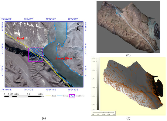
Figure 1.
An illustration of the location and topography of the study site. (a) The location of the study site. (b) The digital ortho model of the study site. (c) The digital elevation model and contour of the study site.
2.2. Data Acquisition
The flight platform was a six-rotor UAV, as shown in Figure 2c, equipped with a full-frame Sony ILCE-7RM4 camera. The detailed parameters of the flight platform and camera system are shown in Table 1. According to the technical requirement that the ground sampling distance (GSD) of the UAV image is 2 cm, the designed flight routes are shown in Figure 2a, where the relative flight altitude was 130 m, and the overlap of heading and side direction were 80% and 60%, respectively. During the experiment period, the same flight routes were used twice to collect UAV data. The first acquisition was on 22 June 2021, and a total of 182 images were acquired. The second collection time was 15 July 2021, and a total of 184 images were obtained.
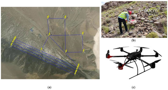
Figure 2.
UAV data acquisition. (a) The flights of the study site. (b) The spray-painted stone. (c) The six-rotor flight platform.

Table 1.
The parameters of the flight platform and camera system.
In order to evaluate the difference between the two cycle models, we selected stones of different sizes within the study site to be painted red, and measured their spatial positions using GNSS-RTK, as shown in Figure 2b.
3. Methodology
The geometric registration of multi-temporal 3D models is to define and solve the transformation model parameters from the vertices of the registered 3D models to the spatial location of the based 3D models. The main process consists of three steps:
- (1)
- The 3D model feature points are extracted from the texture image by the interest point operator, and their position information is computed.
- (2)
- The feature vector of spatial-feature points consists of the image information around the feature points, which are used to match the corresponding points.
- (3)
- According to the corresponding position of the spatial-feature points, the transformation model parameters between models are estimated, than the new transformation model is used to update the spatial location information of the 3D model to be registered.
3.1. Spatial-Feature-Point Extraction
The research object of this paper was a 3D model, which contained data including vertices, triangulated-mesh connecting vertices, and texture-image data corresponding to vertices, as shown in Figure 3a.
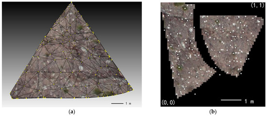
Figure 3.
The composition of the 3D model. (a) The vertices of the 3D model and the triangulation connecting the vertices. (b) The texture image of the 3D model and the texture coordinates corresponding to the vertices.
In Figure 3a, the yellow circles are vertices in the 3D model data, which are connected by black lines to form a triangulation. Each vertex corresponds to a unique normalized 2D texture coordinate, as shown by the white origin in Figure 3b. Then, the corresponding 2D texture coordinates, which are the normalized coordinates of the feature points in the texture image, and 3D vertices are rendered to form a regular 3D model.
The prerequisite of 3D model registration is to obtain high-precision spatial-feature points and their corresponding spatial positions. However, the conventional method of extracting image feature points directly extracts the coordinates of 2D image points, and then recovers their spatial positions based on the SfM pipeline algorithm [27]. Since texture images of 3D model data are irregular images, as shown in Figure 3b, the direct transformation relationship between texture coordinates and their spatial coordinates cannot be directly formed. Therefore, we propose a spatial feature-point-extraction method that can calculate the corresponding spatial positions of feature points on texture images.
Firstly, feature points are extracted from texture images. The scale-invariant feature transform (SIFT) feature has been widely used in the field of feature extraction because of its advantages of invariant to lighting, scale, and rotation changes and can overcome affine image changes [28]. In this paper, SIFT feature points are first extracted from texture images, and their image coordinates are normalized to texture coordinates, as shown in Equation (1).
where and represent the width and height of the texture image (in pixels), respectively. and represent the normalized texture coordinates.
Secondly, the plane coordinates of feature points are interpolated. The normalized texture coordinates of each triangle were searched to obtain the texture vertex coordinates of the triangles. A schematic diagram of a triangle and model triangle is shown in Figure 4.
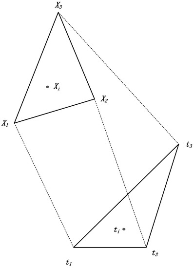
Figure 4.
The mapping relationship between texture triangles and model triangles.
In Figure 4, , , and are the three normalized vertex coordinates of the texture triangle, respectively. , , and are the spatial plane coordinates of the model triangle, respectively. is the normalized texture position corresponding to the extracted feature point. is the spatial position corresponding to . According to the corresponding relationship between the model triangle and the texture triangle, the plane coordinates of texture triangle and model triangle are defined as a 2D affine transformation, which can be expressed as Equation (2).
where are 2D affine-transformation parameters.
The three normalized texture coordinates of the texture triangle and the vertex plane coordinates of the corresponding model triangle are put into Equation (2). After finishing, which can be expressed as:
where , , .
Based on the least-squares adjustment method, the affine-transformation parameters in Equation (3) can be obtained from Equation (4).
All the spatial-feature points obtained by matching are considered as equal-weighted observations, and their corresponding stochastic models are defined as an identify matrix, as shown in Equation (4) for . Affine-transformation parameters can be estimated based on Equation (4). Then, according to affine-transformation parameters and Equation (2), the corresponding space plane coordinates of feature point can be calculated.
Thirdly, the feature-point elevation coordinate is fitted. The vertex coordinates of the model triangle are defined as planes, and the elevation coordinates of the feature point can be obtained by interpolation in the plane after fitting. If the spatial coordinates of the model triangle vertices are , , and , respectively, and the spatial coordinates of the feature points are , then the above four points are in the same plane, which can be expressed as follows:
Equation (5) can be expressed as:
After obtaining the plane coordinates of the feature point, the elevation coordinates of the feature point can be fitted by Equation (6).
3.2. Spatial-Feature-Point Matching
When the feature points of all 3D-model texture images are extracted and their spatial positions are calculated, it is necessary to establish the corresponding relationship between the spatial-feature points of the base 3D model and the spatial-feature points of the 3D model to be registered. Based on the 128-dimension normalized feature vector of SIFT points, the similarity value of the feature vector is obtained after calculating the Euclidean distance, and then it is determined whether the two feature points are corresponding points [28]. In conventional image-matching, the feature points and feature vectors of image A and B are obtained, respectively, and then the similarity between the feature points set of image A and image B are determined successively to complete the two-view image matching. After the feature points and feature vectors of a batch 3D model are completely acquired, the exhaustive search and matching method cannot be realized due to the large amount of data. Therefore, this paper adopts the axis-aligned bounding-box (AABB) search method to match the corresponding points between the feature points of the base 3D model and the feature points of the 3D model to be registered.
After extracting the feature points of the base 3D models, the set of their spatial-feature points is generated, as shown by the blue dots in Figure 5a. In the same way, the spatial-feature-point set of the model to be registered is generated, as shown in Figure 5b. The set of spatial-feature points in Figure 5a is evenly divided into AABB bounding boxes, so that the number of feature points contained in each bounding box is less than a threshold (value 3000), as shown in the bounding box set in Figure 5a. Then, according to the prior knowledge r of the positioning error between the base model and the model to be registered, the bounding box is expanded by r to form the search bounding box for the set of feature points to be registered. After the similarity matching between the bounding box and the searching bounding box is completed, a complete list of corresponding points between the base feature points and the feature points to be registered can be obtained.
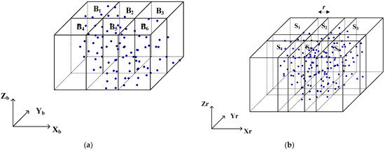
Figure 5.
The AABB bounding box of the search range. (a) The bounding box of the base model space feature points. (b) The searching bounding box of the model space feature points to be registered.
3.3. Registration Model Solution
The geometric transformation model from the vertex of the registered 3D model to the vertex of the base 3D model can be defined as 3D similarity transformation, as shown in Equation (7).
where is the vertex position of the model to be registered and is the corresponding vertex position of the base model. and represents the rotation matrix and the translation from the vertex of the model to be registered to the base model, respectively. represents the scale factor from the vertex of the model to be registered to the base model, and when , Equation (7) becomes a 3D rigid transformation model.
The detailed definition of rotation matrix in Equation (7) is shown in Equation (8).
where are the rotation angle of the rotation matrix .
When a sufficient number of corresponding spatial points are obtained, the Levenberg–Marquardt (LM) algorithm [29] is used for solving non-linear squares problems, and the seven transformation parameters of Equation (7) can be obtained. The open source library “levmar” [30] of the LM algorithm is used to solve the transformation parameters. However, the initial corresponding spatial-feature points obtained by the similarity of feature vectors inevitably contain incorrect correspondences, which are usually referred to as outliers. Therefore, the random sampling consistency algorithm (RANSAC) is adopted to eliminate the outliers and robustly obtain the transformation model parameters [31]. Finally, the estimated model parameters are used to transform all vertices of the registered model to complete the geometric registration.
3.4. Data Processing
After acquiring multi-temporal UAV images and position and orientation system (POS) data, the software of “Context Capture V10.16.0.75” was used for 3D reconstruction to obtain 3D models. Then the feature points of the 3D model were extracted and their corresponding spatial positions were calculated based on the method in Section 3.1. Thirdly, the spatial-feature points were initially matched to obtain the initial correspondence based on the method in Section 3.2. Fourthly, the model transformation parameters from the registration model to the base 3D model were estimated based on the initial correspondence, and all vertices of the registered 3D model were updated based on the method in Section 3.3. The workflow of the data processing is shown in Figure 6.
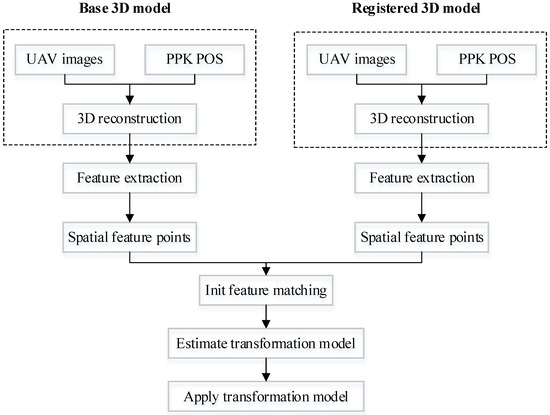
Figure 6.
The workflow of data processing.
4. Experiment Results and Discussions
To verify the effectiveness of the algorithm, we selected seven stones of different sizes in the study area and applied red paint to their surfaces. The distribution of the stones is shown in Figure 7.
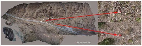
Figure 7.
The 3D model of the study site and the spray-painted stones.
C1–C7 in Figure 7 represent the numbering of the seven stones. The positions of the seven stones were accurately measured by GNSS-RTK equipment. Before the second period of data acquisition, the positions of the seven stones were changed and their spatial positions were measured again, and then the UAV image data were collected. The purpose of the experiment was to evaluate the positioning accuracy of multi-temporal 3D models geometric registration by the moving positions of the seven stones.
4.1. Distribution and Correspondence Analysis of Spatial-Feature Points
The number and distribution of spatial-feature points are the basic conditions for 3D model geometric registration. Firstly, the feature points were extracted from the texture images in the 3D model, and then the spatial positions of the feature points were calculated based on the triangulation of the 3D model to generate the corresponding spatial-feature points. Figure 8 shows the feature-point-extraction results of two texture images.
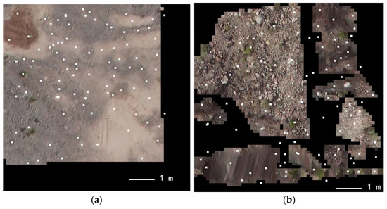
Figure 8.
The distribution of feature points in texture images. (a) A continuous texture image. (b) A fragmented texture image.
The white dots in Figure 8 represent the extracted feature points, of which the feature points extracted in Figure 8a were evenly distributed and not significantly different from those of the conventional image. In Figure 8b, due to the fragmentation of texture images, many feature points were distributed in the non-textured image area. Obviously, these feature points were invalid and needed to be eliminated in the feature-matching process. According to the analysis of feature-point-extraction results in Figure 8, although 3D texture images are irregular and fragmented, a sufficient number of feature points could still be extracted. After extracting all the feature points of the lowest-level model, the spatial positions of the feature points were calculated, and the planar feature points were converted into spatial-feature points. The spatial-feature points were superimposed and displayed with the 3D grid model, as shown in Figure 9.
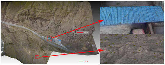
Figure 9.
The distribution of feature points in the mesh model.
The green dots in the left of Figure 9 are the extracted spatial-feature points, which were uniformly distributed on the surface of the mesh model. The right side of Figure 9 shows the enlarged display of the red box. Analysis from the visual performance showed that the extracted spatial-feature points were strictly fitted to the surface of the mesh, and their planar positions and elevation interpolation results were consistent with the actual situation, and were reasonable. After obtaining the spatial-feature points, the initial similarity determination and 3D model geometric registration were performed to obtain the corresponding points in different stages, as shown in Figure 10.
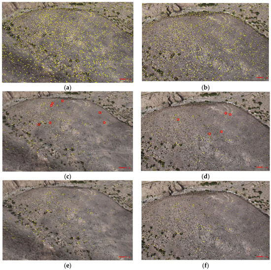
Figure 10.
The corresponding distribution of spatial-feature points, the yellow dots in the figure are the spatial-feature points. (a) The initial spatial-feature points extracted. (c) The initial correspondence of spatial-feature points, with incorrect correspondence in the red box. (e) The fine correspondence of spatial-feature points after registration. (b,d,f) corresponds to (a,c,e) and are the results of the second-cycle data.
The yellow dots in Figure 10a,b represent the distribution of spatial-feature points extracted from the 3D model in two periods, respectively, which were evenly distributed but had no correspondence between spatial-feature points. Figure 10c,d shows the initial matching correspondence of the spatial-feature points for the two periods’ data, from which it can be seen that it still contained a certain number of outlier points, as shown in the red-boxed area. Figure 10e,f shows the final correspondence of the spatial-feature points obtained after model registration. Compared with Figure 10c,d, the outliers existing in the initial corresponding spatial-feature points have been eliminated. After statistics, the number of spatial-feature points extracted from the data in the two periods was 100,834 and 93,751, respectively. After similarity-determination, a total of 4914 initial corresponding points were obtained. A total of 2816 final corresponding spatial points were obtained after the two periods of 3D model registration. Based on the analysis of the above results, it is possible to obtain sufficient and evenly distributed corresponding points by extracting spatial-feature points from the multi-period 3D model.
4.2. Geometric-Registration-Accuracy Analysis of Spatial-Feature Points
A total of three methods are used to generate 3D models for evaluating the relative geometric positioning accuracy of multi-temporal 3D models. The first method is to generate 3D models based on low-precision UAV airborne POS data. The second method uses post-processed kinematic (PPK) technology to obtain high-precision position at the time of image acquisition, and uses a GPS-support method to complete 3D reconstruction to obtain 3D models. The third method uses the 3D-model alignment method proposed in this paper, and performs vertex updates on the 3D model to be aligned based on the model-alignment parameters. The spatial-feature points of the above three types of 3D models were extracted, respectively, and the corresponding points of the final spatial features were obtained. The positions of the spatial-feature points in the base 3D model were subtracted from the positions of those in the 3D model to be aligned to obtain any residual positioning errors, and the results are shown in Figure 11.
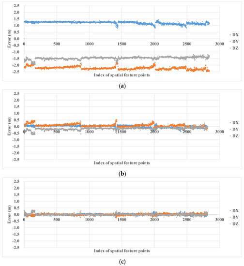
Figure 11.
The corresponding point residual errors of the spatial-feature points. (a) Results obtained based on UAV airborne POS system. (b) Results obtained based on PPK POS data. (c) Results obtained based on 3D-model automatic registration.
DX, DY, and DZ in Figure 11 represent the position residual errors in X, Y, and Z directions, respectively. The residual error distribution in Figure 11a shows that the positioning accuracy of conventional UAV-borne POS was low, and there were obvious systematic errors among the generated multi-temporal 3D models. When high-precision PPK data was used to generate 3D models, the positioning accuracy of its multi-period 3D models was greatly improved. The relative positioning accuracy of the two temporal 3D models was less than 0.2 m, as shown in Figure 11b. However, the average values in the Y and Z directions were not zero, indicating that a small amount of systematic positioning error still existed in these two directions. The residual errors of the corresponding points of the 3D model after using the geometric alignment of this paper were all close to 0 m, showing a random distribution in Figure 11c. The residual-error accuracy of spatial-feature points obtained by the three methods was calculated, and the results are shown in Table 2.
Table 2.
Comparison of the positioning accuracy of corresponding points for different 3D models.
In Table 2, AVG represents the average error of corresponding points of spatial features, which reflects the systematic error of relative positioning accuracy of multi-temporal 3D models. STD represents the standard deviation, which reflects the internal aggregation of corresponding points of spatial features. Based on the results in Table 2, it can be seen that the overall average error of the 3D model generated from conventional UAV airborne POS data was 2.91 m. The accuracy was low and cannot be directly used for change detection in multi-temporal 3D models. The overall average error of the multi-temporal 3D models generated based on PPK data was better than 0.18 m, but there were still a few systematic errors in the Y and Z directions, which were consistent with the results in Figure 11b. The overall average error of the 3D-model alignment method proposed in this paper was almost equal to 0 m. After compensation by the transformation parameters, the overall STD of the corresponding points was reduced from 0.36 m to 0.14 m. In contrast, the geometric registration of multi-temporal 3D models based on spatial-feature points proposed in this paper can effectively eliminate the spatial location differences among 3D models and obtain a unified spatial reference.
4.3. Accuracy Analysis of 3D Model after Registration
In order to further evaluate the positioning error between the registered 3D model and the base 3D model, we accurately measured the displacement of seven spray-painted stones between the two sequential 3D models.
Figure 12 shows the screenshots of the sprayed stones numbered C1 and C5 in the two sequential 3D models. The GNSS-RTK equipment was used to measure the spatial position of the sprayed stones before the two UAV data collections, and their spatial displacement was calculated and used as the true value. Using the same three 3D model data as in Figure 11, the displacement of the sprayed stones in the sequential 3D model was calculated after manually measuring their spatial position in the 3D model. The actual displacement obtained from GNSS-RTK equipment was subtracted from the model displacement measured manually to obtain the difference in displacement of the seven sprayed stones, and the results are shown in Table 3.
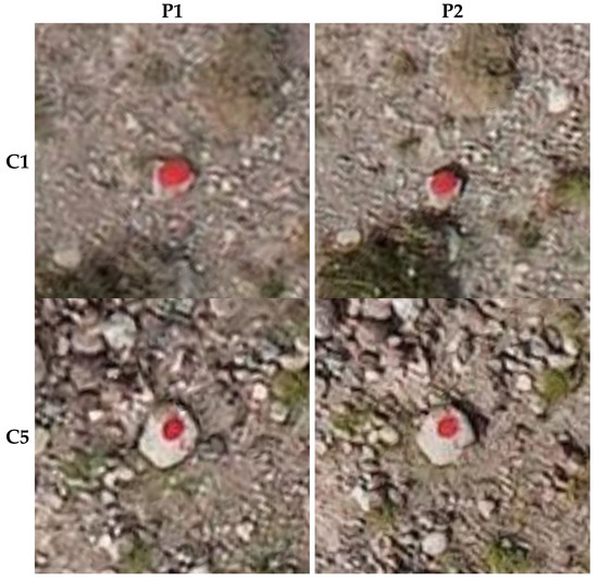
Figure 12.
The sprayed stones in the two sequential 3D model. P1 represents the 3D of the first period, and P2 represents the second period.
Table 3.
The displacement and difference of the sprayed stones in the two sequential 3D models.
The GPS column in Table 3 shows the actual spatial displacement of the sprayed stones. Based on analysis of the results in Table 3, the sequential 3D model generated by conventional POS data shows that the average value of the difference in spatial displacements was −2.47 m, far exceeding the actual spatial displacements of the sprayed stones. So, 3D models generated based on conventional POS data cannot be directly used for ground object change detection. The average value of the spatial-displacement difference was reduced to 0.08 m after using PPK data, which is about three times the GSD. The results show that the multi-period 3D model generated by PPK data can be localized and discovered when the spatial-location-change value of ground objects exceeds three times the GSD. In contrast, the average of the spatial displacement difference was as low as 0.01m for the model-registration method in this paper. The results in Table 3 show that the relative distance measurement error of the aligned 3D model was less than 0.01 m. The results show that the 3D model generated based on the method in this paper has a highly uniform spatial reference for the multi-temporal 3D models and can be directly applied to the change detection of the multi-temporal 3D models.
5. Conclusions
In this paper, we propose a fully automatic 3D model registration method, which converts 2D feature points extracted from the highest resolution texture image of the model into 3D spatial-feature points, and solves the model-transformation parameters of the 3D model to be aligned with respect to the base 3D model, and then establishes a unified spatial reference for multi-temporal 3D models. The experimental results show that the multi-temporal 3D models generated by high-precision PPK data combined with GPS-support method can locate ground object displacement that is more than three times that of the GSD of the UAV image. In comparison, the average value of the difference between the measured ground object displacement and the actual object displacement was 0.01 m for the 3D model generated by the method in this paper. This method does not need to measure GCPs at each data acquisition to make a multi-time series 3D model with a uniform spatial reference. For periodic dynamic inspection tasks, it has the great advantage of saving project cost and economic cost.
Author Contributions
Conceptualization, H.S.; methodology, H.S. and C.R.; software, C.R.; validation, G.L. and Z.L.; formal analysis, G.J.; investigation, G.L.; resources, G.L.; data curation, H.S.; writing—original draft preparation, C.R.; writing—review and editing, C.R.; visualization, H.S.; supervision, Z.L.; project administration, H.S.; funding acquisition, C.R. All authors have read and agreed to the published version of the manuscript.
Funding
This research was funded by the Northwest Engineering Corporation Limited Major Science and Technology Projects, grant number XBY-ZDKJ-2020-08, and the National Natural Science Foundation of China, grant number (41801383). The APC was funded by 41801383.
Institutional Review Board Statement
Not applicable.
Informed Consent Statement
Not applicable.
Data Availability Statement
The data presented in this study are available on request from the corresponding author.
Conflicts of Interest
The authors declare no conflict of interest.
References
- Mathews, A.J. A practical UAV remote sensing methodology to generate multispectral orthophotos for vineyards: Estimation of spectral reflectance using compact digital cameras. Int. J. Appl. Geospat. Res. 2015, 6, 65–87. [Google Scholar] [CrossRef]
- Lu, P.; Catani, F.; Tofani, V.; Casagli, N. Quantitative hazard and risk assessment for slow-moving landslides from Persistent Scatterer Interferometry. Landslides 2014, 11, 685–696. [Google Scholar] [CrossRef]
- Abdulla, A.R.; He, F.; Adel, M.; Naser, E.S.; Ayman, H. Using an unmanned aerial vehicle-based digital imaging system to derive a 3D point cloud for landslide scarp recognition. Remote Sens. 2016, 8, 95. [Google Scholar] [CrossRef]
- Conforti, M.; Mercuri, M.; Borrelli, L. Morphological changes detection of a large earthflow using archived images, LiDAR-derived DTM, and UAV-based remote sensing. Remote Sens. 2020, 13, 120. [Google Scholar] [CrossRef]
- Komarek, J.; Klouček, T.; Prošek, J. The potential of Unmanned Aerial Systems: A tool towards precision classification of hard-to-distinguish vegetation types? Int. J. Appl. Earth Obs. Geoinf. 2018, 71, 9–19. [Google Scholar] [CrossRef]
- Klouek, T.; Komárek, J.; Surov, P.; Hrach, K.; Vaíek, B. The use of UAV mounted sensors for precise detection of bark beetle infestation. Remote Sens. 2019, 11, 1561. [Google Scholar] [CrossRef]
- Castilla, F.J.; Ramón, A.; Adán, A.; Trenado, A.; Fuentes, D. 3D sensor-fusion for the documentation of rural heritage buildings. Remote Sens. 2021, 13, 1337. [Google Scholar] [CrossRef]
- Lucieer, A.; Jong, S.; Turner, D. Mapping landslide displacements using structure from motion (SfM) and image correlation of multi-temporal UAV photography. Prog. Phys. Geogr. 2014, 38, 97–116. [Google Scholar] [CrossRef]
- Guzzetti, F.; Mondini, A.C.; Cardinali, M.; Fiorucci, F.; Santangelo, M.; Chang, K.T. Landslide inventory maps: New tools for an old problem. Earth-Sci. Rev. 2012, 112, 42–66. [Google Scholar] [CrossRef]
- Ewertowski, M.; Tomczyk, A.; Evans, D.; Roberts, D.; Ewertowski, W. Operational framework for rapid, very-high resolution mapping of glacial geomorphology using low-cost unmanned aerial vehicles and structure-from-motion approach. Remote Sens. 2019, 11, 65. [Google Scholar] [CrossRef]
- Rakha, T.; Gorodetsky, A. Review of unmanned aerial system (UAS) applications in the built environment: Towards automated building inspection procedures using drones. Autom. Constr. 2018, 93, 252–264. [Google Scholar] [CrossRef]
- Kohv, M.; Sepp, E.; Vammus, L. Assessing multitemporal water-level changes with uav-based photogrammetry. Photogramm. Rec. 2017, 32, 424–442. [Google Scholar] [CrossRef]
- Huang, F.; Yang, H.; Tan, X.; Peng, S.; Tao, J.; Peng, S. Fast reconstruction of 3D point cloud model using visual SLAM on embedded UAV development platform. Remote Sens. 2020, 12, 3308. [Google Scholar] [CrossRef]
- Smith, M.; Carrivick, J.; Quincey, D. Structure from motion photogrammetry in physical geography. Prog. Phys. Geogr. 2015, 40, 247–275. [Google Scholar] [CrossRef]
- Westoby, M.J.; Brasington, J.; Glasser, N.F.; Hambrey, M.J.; Reynolds, J.M. ‘Structure-from-Motion’ photogrammetry: A low-cost, effective tool for geoscience applications. Geomorphology 2012, 179, 300–314. [Google Scholar] [CrossRef]
- Stathopoulou, E.K.; Welponer, M.; Remondino, F. Open-source image-based 3D reconstruction pipelines: Review, comparision and evaluation. ISPRS-Int. Arch. Photogramm. Remote Sens. Spat. Inf. Sci. 2019, XLII-2/W, 331–338. [Google Scholar] [CrossRef]
- Ren, C.; Zhi, X.; Pu, Y.; Zhang, F. A multi-scale UAV image matching method applied to large-scale landslide reconstruction. Math. Biosci. Eng. 2021, 18, 2274–2287. [Google Scholar] [CrossRef]
- Le, V.C.; Cao, X.C.; Long, N.Q.; Le, T.; Anh, T.T.; Bui, X.N. Experimental investigation on the performance of DJI Phantom 4 RTK in the PPK Mode for 3D mapping open-pit mines. Inz. Miner. 2020, 1, 65–74. [Google Scholar]
- Long, N.; Goyal, R.; Bui, L.; Cao, C.; Canh, L.; Quang Minh, N.; Bui, X.-N. Optimal choice of the number of ground control points for developing precise DSM using light-weight UAV in small and medium-sized open-pit mine. Arch. Min. Sci. 2021, 66, 369–384. [Google Scholar]
- Ren, C.; Shang, H.; Zha, Z.; Zhang, F.; Pu, Y. Color balance method of dense point cloud in landslides area based on UAV images. IEEE Sens. J. 2022, 22, 3516–3528. [Google Scholar] [CrossRef]
- Troner, M.; Urban, R.; Seidl, J.; Reindl, T.; Brouek, J. Photogrammetry using UAV-mounted GNSS RTK: Georeferencing strategies without GCPs. Remote Sens. 2021, 13, 1336. [Google Scholar] [CrossRef]
- Gong, Y.; Meng, D.; Seibel, E.J. Bound constrained bundle adjustment for reliable 3D reconstruction. Opt. Express 2015, 23, 10771–10785. [Google Scholar] [CrossRef] [PubMed]
- Triggs, B. Bundle Adjustment—A modern synthesis. In Proceedings of International Workshop on Vision Algorithms: Theory & Practice; Springer: Berlin/Heidelberg, Germany, 1999; pp. 298–372. [Google Scholar]
- Troner, M.; Urban, R.; Reindl, T.; Seidl, J.; Brouek, J. Evaluation of the georeferencing accuracy of a photogrammetric model using a quadrocopter with onboard GNSS RTK. Sensors 2020, 20, 2318. [Google Scholar] [CrossRef]
- Taddia, Y.; Stecchi, F.; Pellegrinelli, A. Coastal mapping using DJI Phantom 4 RTK in post-processing kinematic mode. Drones 2020, 4, 9. [Google Scholar] [CrossRef]
- Corominas, J.; Westen, C.V.; Frattini, P.; Cascini, L.; Smith, J.T. Recommendations for the quantitative analysis of landslide risk. Bull. Eng. Geol. Environ. 2014, 73, 209–263. [Google Scholar] [CrossRef]
- James, M.R.; Robson, S.; D"Oleire-Oltmanns, S.; Niethammer, U. Optimising UAV topographic surveys processed with structure-from-motion: Ground control quality, quantity and bundle adjustment. Geomorphology 2017, 280, 51–66. [Google Scholar] [CrossRef]
- Lowe, D. Distinctive image features from scale-invariant key points. Int. J. Comput. Vis. 2003, 60, 91–110. [Google Scholar] [CrossRef]
- Nocedal, J.; Wright, S.J.; Mikosch, T.V.; Resnick, S.I.; Robinson, S.M. Numerical Optimization; Springer: Berlin/Heidelberg, Germany, 1999. [Google Scholar]
- Levmar: Levenberg-Marquardt Nonlinear Least Squares Algorithms in C/C++. Available online: http://users.ics.forth.gr/~lourakis/levmar/ (accessed on 22 October 2020).
- Fischler, M.A.; Bolles, R.C. Random sample consensus: A paradigm for model fitting with applications to image analysis and automated cartography. Read. Comput. Vis. 1981, 24, 381–395. [Google Scholar] [CrossRef]


Publisher’s Note: MDPI stays neutral with regard to jurisdictional claims in published maps and institutional affiliations. |
© 2022 by the authors. Licensee MDPI, Basel, Switzerland. This article is an open access article distributed under the terms and conditions of the Creative Commons Attribution (CC BY) license (https://creativecommons.org/licenses/by/4.0/).