Article

Design and Control of a Pneumatic Muscle Servo Drive Containing Its Own Pneumatic Muscles

by
Dawid Sebastian Pietrala
* and
Pawel Andrzej Laski
Department of Automation and Robotics, Faculty of Mechatronics and Mechanical Engineering, Kielce University of Technology, 25-314 Kielce, Poland
*
Author to whom correspondence should be addressed.
Appl. Sci. 2022, 12(21), 11024; https://doi.org/10.3390/app122111024
Submission received: 5 October 2022 / Revised: 21 October 2022 / Accepted: 26 October 2022 / Published: 31 October 2022
(This article belongs to the Section Mechanical Engineering)

Abstract

:
This article presents static and dynamic characteristics of artificial pneumatic muscles. The research stance and the methodology for their determination are described. A mathematical model of a pneumatic muscle has been proposed, having two inputs—the force generated by the muscle and the displacement of the muscle tip, and one output—the valve control voltage. The quality of object mapping was verified by a mathematical model for various trajectories. Then, the control system for the moment servo drive force was composed of two pneumatic muscles working in opposite directions connected by a toothed belt gear. The servo drive was verified and evaluated.

1. Introduction

A pneumatic muscle is a type of single-acting cylinder which, under the influence of an increase in internal pressure, increases its volume by increasing its diameter while reducing its length. Changing the length of the cylinder is used as a working movement [1]. The basic physical quantities describing the behavior of a muscle in a steady state are internal hypertension p muscle length l and the force generated by the F muscle. In 1957, Dr. Joseph L. McKibben used the pneumatic muscle he had developed to propel his limbs. This muscle consisted of an elastic bladder placed freely inside a braid of inextensible fibers. At the ends, the braid and the bladder were connected which allowed for the transfer of the forces generated by the muscle and the working medium, which was carbon dioxide. This muscle is often referred to as “McKibben’s muscle”. In 1980, the Bridgestone Rubber Company commercialized the pneumatic muscle on a massive scale by introducing a muscle that was an improvement on Dr. McKibben’s design. Currently, pneumatic muscles are mainly offered by two companies: since 1987, Shadow Robot Company has been producing and selling muscles modeled on the McKibben project, while in 1999, Festo, a well-known manufacturer of pneumatic devices, introduced pneumatic muscles that could be tailored to individual applications. It is fundamentally different in structure from McKibben’s muscle. In the Festo project, the braid and the rubber bladder are fused along the entire length of the muscle. The view of the muscle in this version is shown in Figure 1. This solution significantly increases the resistance of the muscle to mechanical damage and increases its durability. However, it has the disadvantage of a lower relative shortening of the muscle and, hence, less effective working movement is generated by the muscle.
Work is underway in many research centers around the world to analyze artificial pneumatic muscles and to determine mathematical models describing their behavior. These models can be broadly divided into static and dynamic, as well as into positional models, where the key is to determine the length of the muscle, and force models, where it is crucial to determine the force generated by the muscle. The first stage of the analysis of pneumatic muscles is often the determination of their static characteristics in the form of isobaric, isotonic and isometric characteristics and their dynamic characteristics in the form of the dependence of the force generated by the muscle on time as the object’s response to a step change in internal pressure. The methodology of their determination and the characteristics of the muscles modeled on the McKibben design, Festo muscles and many original designs are presented, among others, have been previously described [2,3,4,5,6,7,8,9,10,11,12]. In the article [5], Takosoglu and his team presented the research methodology and determined the static characteristics: isobaric, isotonic and isometric of Festo pneumatic muscles and Shadow Robot Company muscles.
In publications describing the static models of muscles, the research mainly concerns the determination of the relationship between internal overpressure, the length of the muscle and the force generated by the muscle in relation to the geometric parameters of the muscle. Research was also carried out on the determination of dynamic models of both McKibben’s and Festo’s muscles, as well as on other structures developed in various research centers, and on the development of positional and force control methods using the presented mathematical models. These issues were extensively discussed, inter alia, in the research of [13,14,15,16,17,18]. Due to the significant friction between the fibers of the braid and between the braid and the rubber bladder, there is a hysteresis phenomenon in the muscles modeled on the McKibben design. It concerns both the shortening of the muscle and the force generated by it. In the case of shortening, the hysteresis manifests itself as the difference between the contraction value ∆l1 at a given internal overpressure and the constant loading force in the case where overpressure was increased, and the contraction value ∆l2 at the same internal overpressure and constant loading force in the case where overpressure was decreased. In the case of the analysis of the force generated by the muscle, the hysteresis refers to the difference between the force F1 generated at a given internal overpressure and constant contraction ∆l in the case where overpressure was increased, and the value of force F2 generated at the same internal overpressure and constant contraction ∆l in the case of overpressure. reduced. This issue is the subject of many studies, e.g., [19,20,21,22,23,24,25].
The analysis presented above shows that Festo is the leading manufacturer of pneumatic muscles. The company produces two types of pneumatic muscles marked MAS and DMSP, each of which is offered in a version with a nominal diameter of dn = 10 mm, dn = 20 mm and dn = 40 mm. This parameter is crucial due to the use of the pneumatic muscle, because its value defines the maximum force F that the muscle is able to generate at a given internal overpressure p. The muscles offered by Festo differ significantly in their structure from the structure developed by Dr. McKibben. In the original design, the rubber bladder was placed freely inside an elastic braid and was connected to it only in two places at the ends of the muscle. On the other hand, the design of Festo has two layers of braid and two layers of a rubber bladder placed alternately and vulcanized together. This design of the drive makes it durable and much more resistant to mechanical damage than a classic muscle. However, the main disadvantage of such a solution is the lower relative contraction of ε, determined according to the relationship (1),
ε = l n l l n 100 %
where ln—nominal length of the muscle at zero overpressure, l—actual length of the muscle. The mentioned negative feature is important from the point of view of the use of pneumatic muscles for the construction of the servo drive. Smaller maximum shortening forces the use of muscles with a greater nominal length in order to develop the same range of servo drive movements, which results in an increase in the geometrical dimensions of both the servo drive and the entire designed manipulator. For this reason, a decision was made to develop and manufacture their own pneumatic muscles with the possibility of initial negative shortening. It was assumed that the designed muscles would have a structural system modeled on McKibben’s muscles, i.e. have a rubber bladder placed freely inside the flexible braid, nominal diameter dn = 20 mm and nominal length ln = 350 mm. Such parameters should ensure the maximum possible muscle contraction of at least x = 100 mmand the maximum working force of at least F = 900 N. Figure 1 shows the view of the developed pneumatic muscle at zero internal overpressure and at internal overpressure equal to p = 0.6 MPa.
In this article, the authors analyze the possibility of building their own artificial pneumatic muscles and their use to build a servo drive that maintains a given moment of force. For this purpose, the article presents the analysis and synthesis of a pneumatic muscle torque servo, built of two pneumatic muscles working in opposite directions and connected by a gear with a toothed belt. This servo drive was used to build a parallel delta manipulator with six degrees of freedom.

2. Materials and Methods
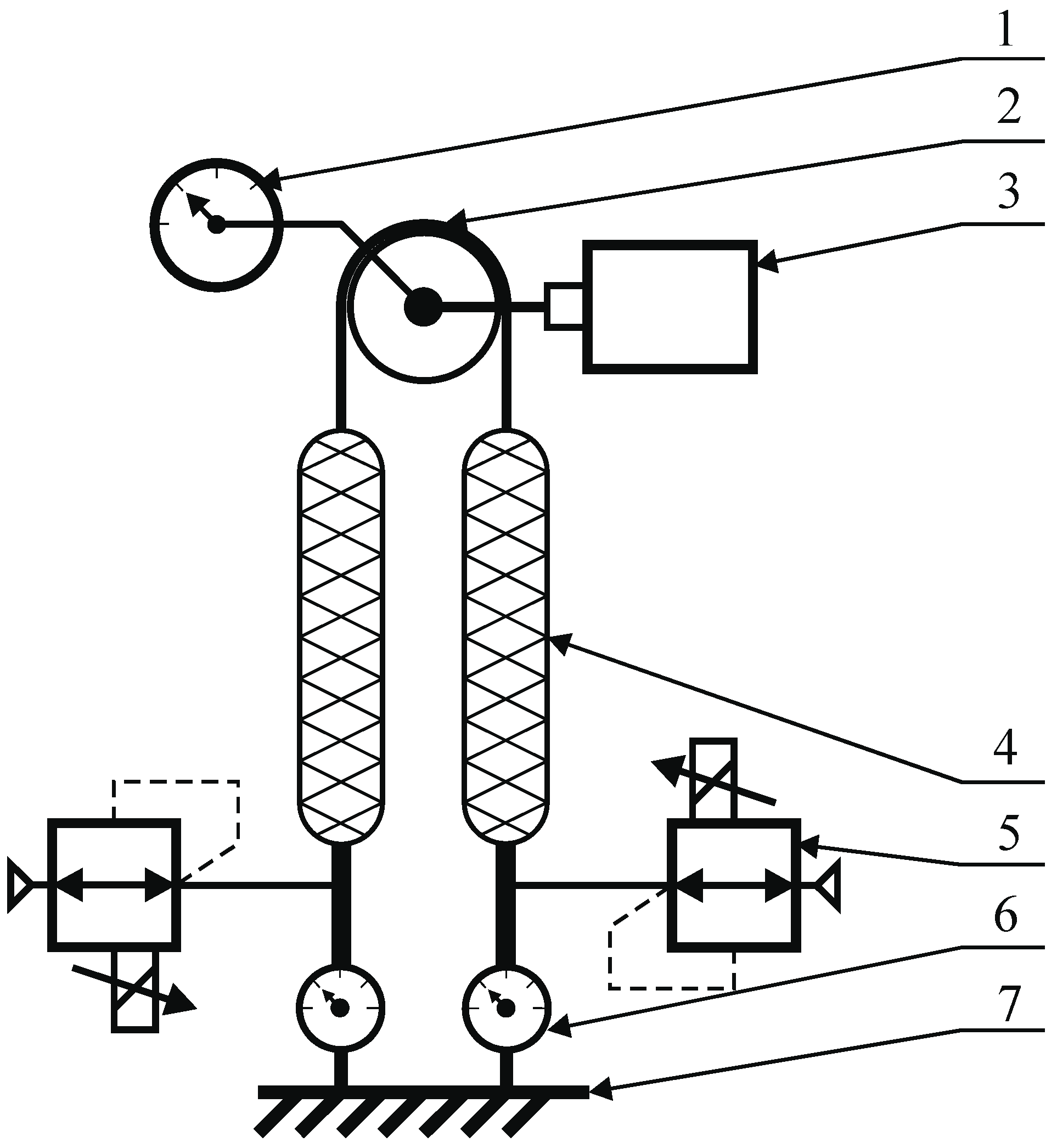
2.1. Test Stand

In order to verify the assumed thesis, first the static and dynamic characteristics of a single muscle were determined. In this servo drive proportional piezoelectric pressure servo valves Hoerbiger Tecno Plus with output pressure were used to supply the muscle with the working medium p = 0−1 MPa and control signal u = 0−10 V. A single muscle, along with its associated valve and connecting line, is the object being analyzed. In steady state, this object is characterized by three quantities: valve servicing voltage u being the input signal for the object and the force generated by the muscle F and muscle tip position x, which are the output signals of the object. When determining all the characteristics, it was assumed that the position of the muscle tip is the difference between the nominal length of the muscle ln and its current length l expressed in millimeters. For the examined muscle, the nominal length was ln = 350 mm. In steady state hypertension prevailing inside the muscle p linearly corresponds to the control signal u by dependence p(MPa) = 0.1 u(V). The relationship between the three quantities characterizing the muscle can be represented as three types of static characteristics: isobaric—the dependence of the position on the loading force, with a constant value of the control voltage for several voltage values x = g(F); u = const, isotonic—dependence of the position on the control voltage at constant loading force, for several strength values x = g(u); F = const and isometric—force dependence on the control voltage, with a constant muscle position, for several position values F = g(u); x = const. The scheme for determining these characteristics is presented in Figure 2. However, the behavior of the object over time can be determined by determining two families of dynamic characteristics, one for each of the object’s output quantities. The first family of dynamic characteristics presents the relationship of muscle position x since t as a response to a step change in the valve control signal u, with constant muscular force F. The second family of characteristics shows the dependence of the force generated by the muscle F since t as a response to a step change in the control signal u with a fixed position of the muscle tip x [13].
In order to determine the characteristics discussed above, a test stand was designed and constructed, the diagram and real view of which are shown in Figure 3. The stand allows testing of a single muscle (4) and a pair of muscles working in opposite directions connected by a toothed belt gear (3) with a pitch diameter dp = 63.66 mm.
The station has an absolute optical encoder (2) with a resolution of 16 bits per revolution enabling determination of muscle displacement with accuracy ∆x = 0.005 mm. The stand has also been equipped with Hoerbiger Tecno Plus pressure servo valves (5) for supplying the muscles with a working medium. In addition, the station is equipped with two strain-gauges (6) with a range ±2 kN with an analog voltage output ±10 V. In order to load muscles with the set force value, the station is equipped with an electric servo drive with a rated power of 400 W and a rated torque of 1.27 Nm with a precise planetary gear ratio i = 70 and maximum arc clearance of 9 arcmin (1) driving the toothed belt transmission. This drive allows for the loading of a single muscle with strength Fmax = 2792 N. In addition, due to the non-linearity of the generated torque in relation to the set electrical current value resulting primarily from the use of planetary gears, an additional control system with a PID type regulator has been implemented to control the muscle loading force. A strain-gauge force sensor was used as the feedback.

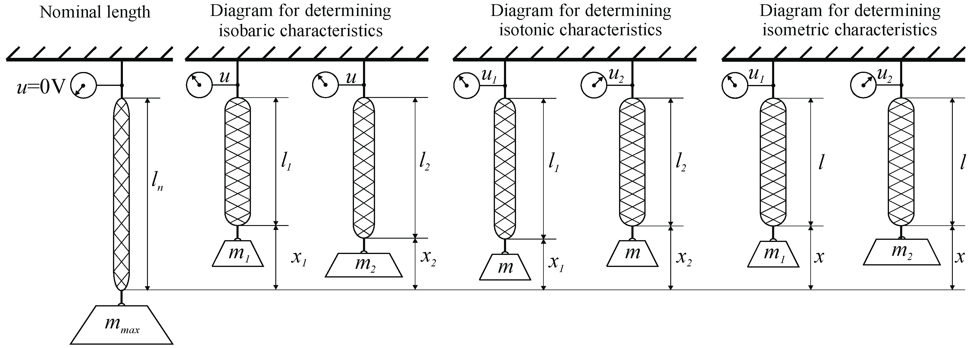
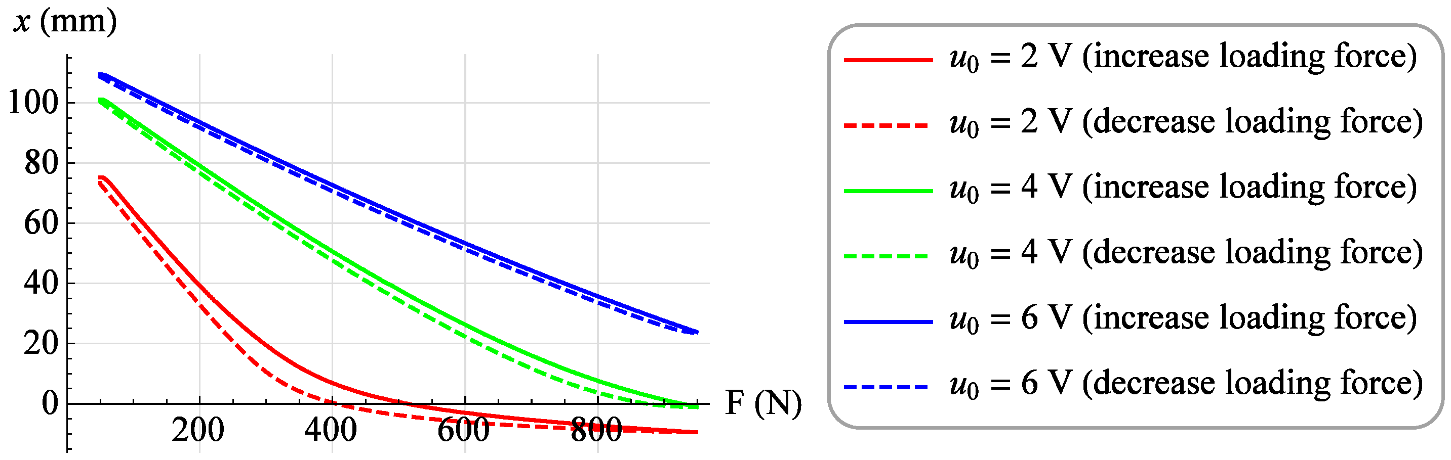
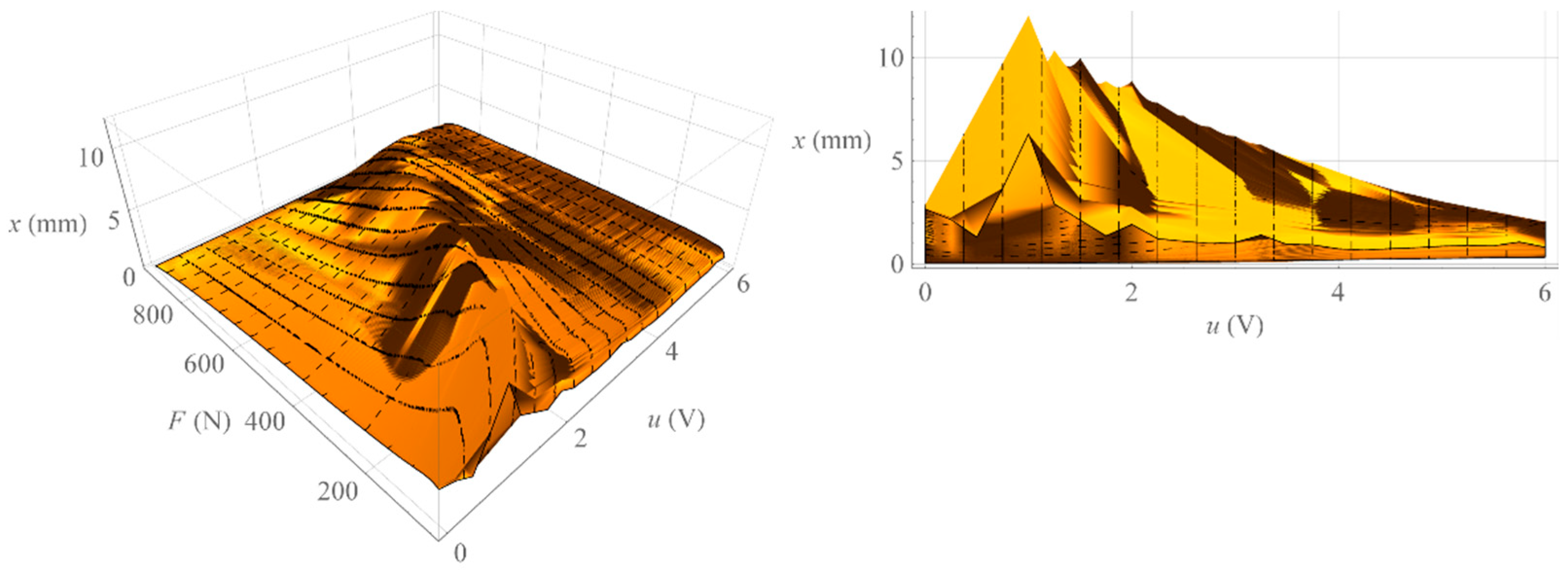
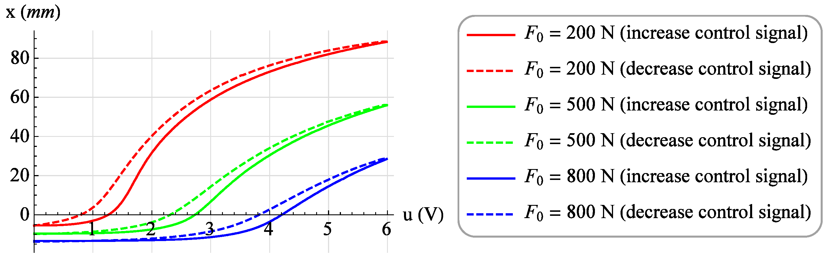
2.2. Static Characteristics

A set of isobaric characteristics was determined for the value of the control signal u from 0 V to 6 V. For each value of the control signal, the value of the loading force F was increased from 50 N to 950 N with a step of 10 N, and after waiting for a period of time equal to 3 seconds, the value of the muscle position x was read. Then, measurements were made at the same control voltage u by reducing the value of the loading force F from 950 N to 50 N with the same step and also, after waiting for a period of time equal to 3 s, the value of the muscle position x was read. As a result, a family of isobaric characteristics was obtained. Figure 4 shows exemplary isobaric characteristics for the values of control voltages u = 2 V, u = 4 V and u = 6 V, when increasing (solid line) and decreasing (dashed line) the loading force F.
Figure 5 shows the surface formed by all isobaric characteristics determined by increasing the loading force (left) and the area formed by all isobaric characteristics determined by decreasing the loading force (right). On the other hand, Figure 6 shows the area representing the amount of mechanical hysteresis for the entire family of isobaric characteristics.
Then, a family of 19 isotonic characteristics were determined for the constant values of the loading forces F from 50 N to 950 N. For each value of the loading force, the value of the control signal u was increased from 0 V to 6 V in steps of 0.1 V, and after waiting for a period of time equal to 3 seconds, the value of the muscle position x was read. Then, with the same loading force F, measurements were made while reducing the value of the control signal u from 6 V to 0 V with the same step. Also, after waiting for a period of 3 seconds, the value of muscle position x was read. Figure 7 shows exemplary isotonic characteristics for the values of the loading forces F = 200 N, F = 500 N and F = 800 N, with increasing (solid line) and decreasing (dashed line) the value of the control signal.
Figure 8 shows the surface formed by all isotonic characteristics determined when increasing the value of the control signal (left) and the surface formed by all isotonic characteristics determined by decreasing the value of the control signal (right). On the other hand, Figure 9 shows the surface representing the amount of mechanical hysteresis for the entire family of isotonic characteristics.
Moreover, a family of 23 isometric characteristics were determined for constant values of the muscle position x from 0 mm to 110 mm with a step of 5 mm. For each position value, the value of the control signal u was increased from 0 V to 6 V with a step of 0.1 V, and after waiting for a period of 3 s, the value of the force generated by muscle F was read. Then, for the same value of muscle position x, measurements were made at decreasing the value of the control signal u from 6 V to 0 V with the same step. Figure 10 shows selected isometric characteristics for the position of the muscle x = 20 mm, x = 50 mm and x = 80 mm for increasing (solid line) and decreasing (dashed line) the value of the control signal.
On the other hand, Figure 11 shows the surface formed by all isometric characteristics determined when increasing the value of the control signal (left) and the surface formed by all isometric characteristics determined when decreasing the value of the control signal (right). On the other hand, Figure 12 shows the surface representing the amount of mechanical hysteresis for the entire family of isometric characteristics.
Analyzing Figure 3, one can notice the difference between the isobaric characteristic when increasing the loading force F and the characteristic when decreasing the loading force F. It is a mechanical hysteresis resulting mainly from the frictional forces between the fibers of the muscle braid and between the braid fibers and the elastic bladder. This phenomenon is also noticeable in the case of other static characteristics. Analyzing the isotonic characteristics presented in Figure 6, it can be seen that for significant values of the loading forces F, the initial increase in the control signal u, and thus the increase in the internal overpressure of the muscle p, does not change the position of the muscle x. On the other hand, when analyzing the isometric characteristics presented in Figure 9, it was noticed that for the constant values of the muscle position x, the value of the force generated by the muscle F changes proportionally to the value of the control signal u. From the above characteristics one can also read the value of the static amplification of the object k. In the case of isometric characteristics, the static gain of the object k(x) expressed as the ratio of the force generated by the muscle F to the control voltage u varies in the range from k min ( 95     mm ) =   17.4     N V to k max ( 0     mm ) =   284.3     N V . However, in the case of isotonic characteristics, the static gain of the object k ( u , F ) expressed as the ratio of the muscle position x to the control voltage u depends on the operating point of the object defined by two parameters. Its minimum value is k min ( 0   V ,     100   N ) =   0.13       mm V and its maximum value k max ( 0.86   V ,     50   N ) =   97.16       mm V .

2.3. Dynamic Characteristics
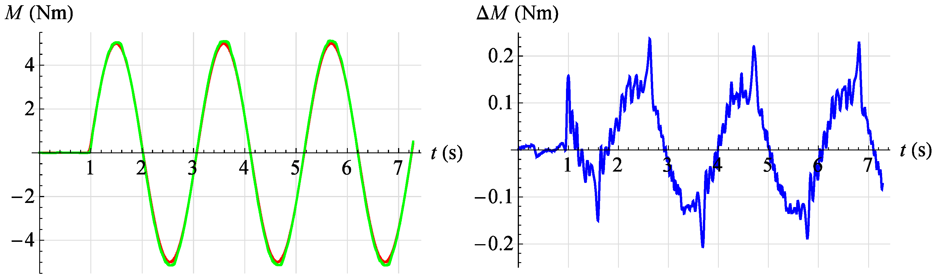
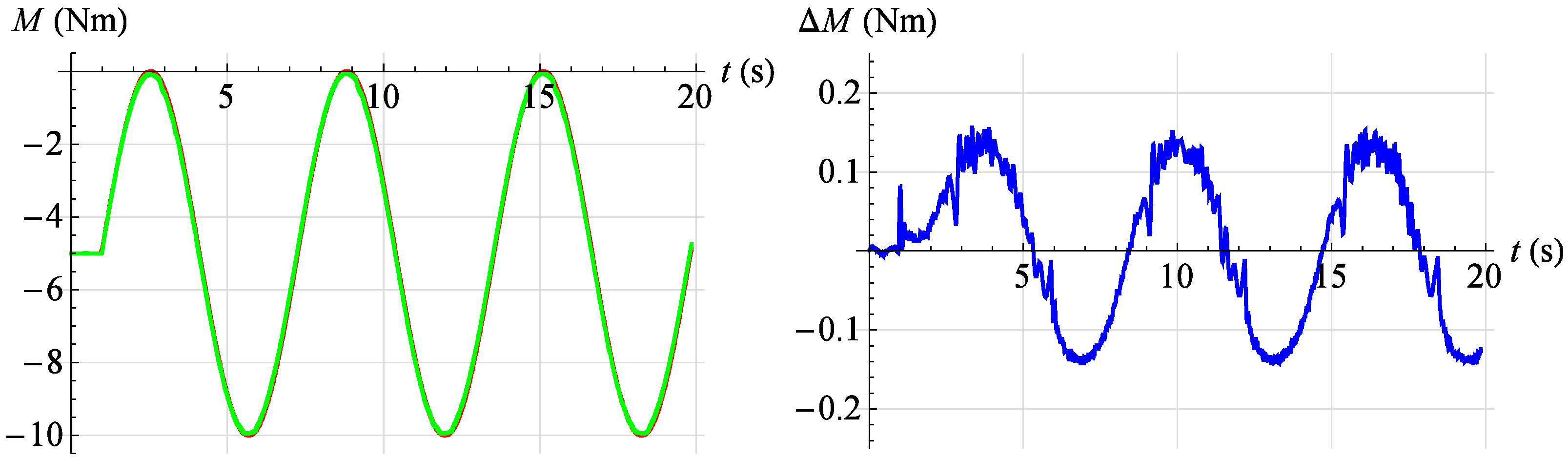
A family of dynamic characteristics was determined in the form of changes in force F as the object’s response to a step change in the valve control signal u, with a constant value of the muscle position x 0 . A series of measurements was performed for 17 different values of the muscle position in the range from 0 mm to 80 mm. The test for a given position value was performed by a step change of the control signal from value u 0   =   1     V to value u n = u 0 + n   0 . 2   V ;     ( n   =   1 ,   2 ,   ,   20 ) . In contrast, the measurement of the force generated by the muscle was carried out for a period of 1 second with a sampling frequency of 1 kHz. Figure 12 (left) shows selected dynamic characteristics for the constant value u n > u 0 of the muscle displacement equal to x 0   =   20     mm . On the other hand, Figure 12 (right) shows selected dynamic characteristics for u n   =   5     V and at different values of muscle displacement.
As before, a family of dynamic characteristics was determined representing the change in force generated by the muscle as a response to a step change of the control signal from value u 0   =   5     V to value u n = u 0   n   0 . 2     V ;     ( n   =   1 ,   2 ,   ,   20 ) . These tests were performed for 17 different values of the muscle position x 0 ranging from 0 mm to 80 mm. The force measurement period and sampling frequency did not change. Figure 13 and Figure 14 (left) shows selected dynamic characteristics with a constant value of the muscle position x 0   =   40     mm . On the other hand, Figure 13 and Figure 14 (right) shows selected dynamic characteristics for u n   =   1     V and at different values of the muscle position.
Analyzing the dynamic characteristics in the form of changes in the force generated by the muscle as a response to a step change in the control signal at a constant position of the muscle, presented in Figure 13 and Figure 14, it was observed that the behavior of the tested object in the vicinity of a given operating point corresponds to the behavior of a second-order object of an oscillating nature.

3. Results

3.1. Mathematical Model of a Pneumatic Muscle

A mathematical model describing the dynamic relationship between the force generated by the muscle was started F a and the control signal u a and current muscle position x a . Analyzing the dynamic characteristics presented in Section 1, it was noticed that the behavior of the object in the vicinity of a given work point can be described by a second order differential equation with constant coefficients. In the general case, the work point of the object can be fully defined using two parameters: the force generated by the muscle F a and the position of the muscle tip x a . Analyzing static characteristics presented in Section 2 it was noticed that the dependence of the force generated by the muscle on the control signal is close to linear over the full range of the muscle F a ( u a , x a ) a ( x a ) u a + F a , 0 for x a 0   mm ;   80   mm . Therefore, in order to base the model, it is enough to linearize only the static characteristics describing the relationship between the muscle position and the control signal. Therefore, in this case, the muscle work point can be defined with one parameter—the current muscle position x a expressed in absolute coordinates. During the tests, the muscle was kept in initial tension, giving the initial value of the control signal u a , 0 constant for each work point. This resulted in the muscle generating an initial value of strength F a , 0 . The model describing the behavior of the object in the surroundings of a given point is shown by the formula (2),
F ¨   +   b F ˙   +   c F   =   d u ; u ( 0 ) = u a , 0 = 1   V ; F ( 0 ) = F a , 0 ( x a , u a , 0 ) ;     F ˙ ( 0 ) = 0 ;    
where: F—the force generated by the muscle in the coordinates of the deviations in the vicinity of the working point, u—control signal in the coordinates of the deviations around the working point, F a , 0 —initial value of the force in absolute coordinates, x a —constant muscle position, u a , 0 —initial value of the control signal in absolute coordinates, b ,   c ,   d —model coefficients. Out of all those designated in Section 2 dynamic characteristics depicting the dependence of force F on time t as a response to a step change in the control signal from a value u a , 0 = 1   V to a value u a , n = 5   V with a stable muscle position x a , a set of 17 characteristics was selected, one for each work point of the object. Then, using the Wolfram Mathematica software, the equation solution was matched to each characteristic (2) represented by the formula (3),
F ( t ) = e 1 2 ( b + b 2 4 c ) t ( b ( 1 + e b 2 4 c t ) ( c F a , 0 ( x a , 0 ) d u u a , 0 ) + b 2 4 c ( c ( 1 + e b 2 4 c t ) F a , 0 ( x a , 0 ) + ( 1 + 2 e 1 2 ( b + b 2 4 c ) t e b 2 4 c t ) ( d u + u a , 0 ) ) ) 2 b 2 4 c c
The results of this match for several selected step responses are shown in Figure 15 and Figure 16. On the left, a solid line indicates the actual response of the object and a dashed line indicates the response of the fitted model. However, the right side shows the absolute match error.
As a result of matching the model to the object characteristics, a set of 17 values b ,   c ,   d was obtained for each model coefficient F a , 0 and for the initial condition. Then, individual values for a given coefficient were approximated by the fifth-degree polynomial of one variable. After substituting the obtained polynomials for Equations (2) and (3), a final model was obtained describing the behavior of the object (4) and its inverse model described by the dependence (5) in the form of a second-order differential equation with variable coefficients that can be used to build a force moment servo drive.
F ( t ) = e 1 2 ( b ( x a , 0 ) + b ( x a , 0 ) 2 4 c ( x a , 0 ) ) t ( b ( x a , 0 ) ( 1 + e b ( x a , 0 ) 2 4 c ( x a , 0 ) t ) ( c ( x a , 0 ) F a , 0 ( x a , 0 ) d ( x a , 0 ) u u a , 0 ) + b ( x a , 0 ) 2 4 c ( x a , 0 ) ( c ( x a , 0 ) ( 1 + e b ( x a , 0 ) 2 4 c ( x a , 0 ) t ) F a , 0 ( x a , 0 ) + ( 1 + 2 e 1 2 ( b ( x a , 0 ) + b ( x a , 0 ) 2 4 c ( x a , 0 ) ) t e b ( x a , 0 ) 2 4 c ( x a , 0 ) t ) ( d ( x a , 0 ) u + u a , 0 ) ) ) 2 b ( x a , 0 ) 2 4 c ( x a , 0 ) c ( x a , 0 )
F ¨   +   b ( x a ) F ˙   +   c ( x a ) F   =   d ( x a ) u + u a , 0
It was considered reasonable to make a quantitative comparison between the developed dynamic model and the static model presented by the relationship F a = g ( x a , u a ) being the de facto static characteristics of the object. The two models were verified and compared. For this purpose, inverse models were used to control the object according to the diagram on Figure 17.
A set force value was introduced into the dynamic inverse model F a , z a d in the absolute coordinates the muscle is to work out, the current value of the force generated by the muscle F a , in absolute coordinates, and the current position of the muscle x a , in absolute coordinates, specifying the working point of the object. The value of force in the coordinates of deviations was determined as the difference between the set value and the actual value F = F a , z a d F a . The model, however, generated a control signal u a = u + u a , 0 fed to the control valve. Similarly to the static inverse model, a set force value was introduced F a , z a d and current muscle position value x a , and the model generated a control signal u a . In Figure 18 and Figure 19, results of the verification of both developed models are presented. The charts on the left show in red the set value of the force which the muscle was to develop, in green the measured value of the force generated by the muscle while controlling the static model and the blue color is the measured value of the force generated by the muscle when controlling the dynamic model. However, on the right side there are control deviations using both models. In Figure 18, the verification results for the set signal described by the dependence are presented F a , z a d   =   50 sin t + 400 with a stable muscle position x a   =   20   mm .
On Figure 19 the verification results for the set signal described by the dependence are presented F a , z a d   =   50 sin t + 200 with a stable muscle position x a   =   50   mm .
Analyzing the results of the work of both mathematical models, it was found that they reflect the behavior of the object in a highly satisfactory manner, and it should be assumed that each of them can be successfully used to build a torque servo drive. However, a direct comparison of the two models indicates that the dynamic model provides a much better representation of the object. Therefore, the dynamic model, although its development requires much more work than developing a static model, was chosen as the basis for the servo drive moment force discussed in Section 3.

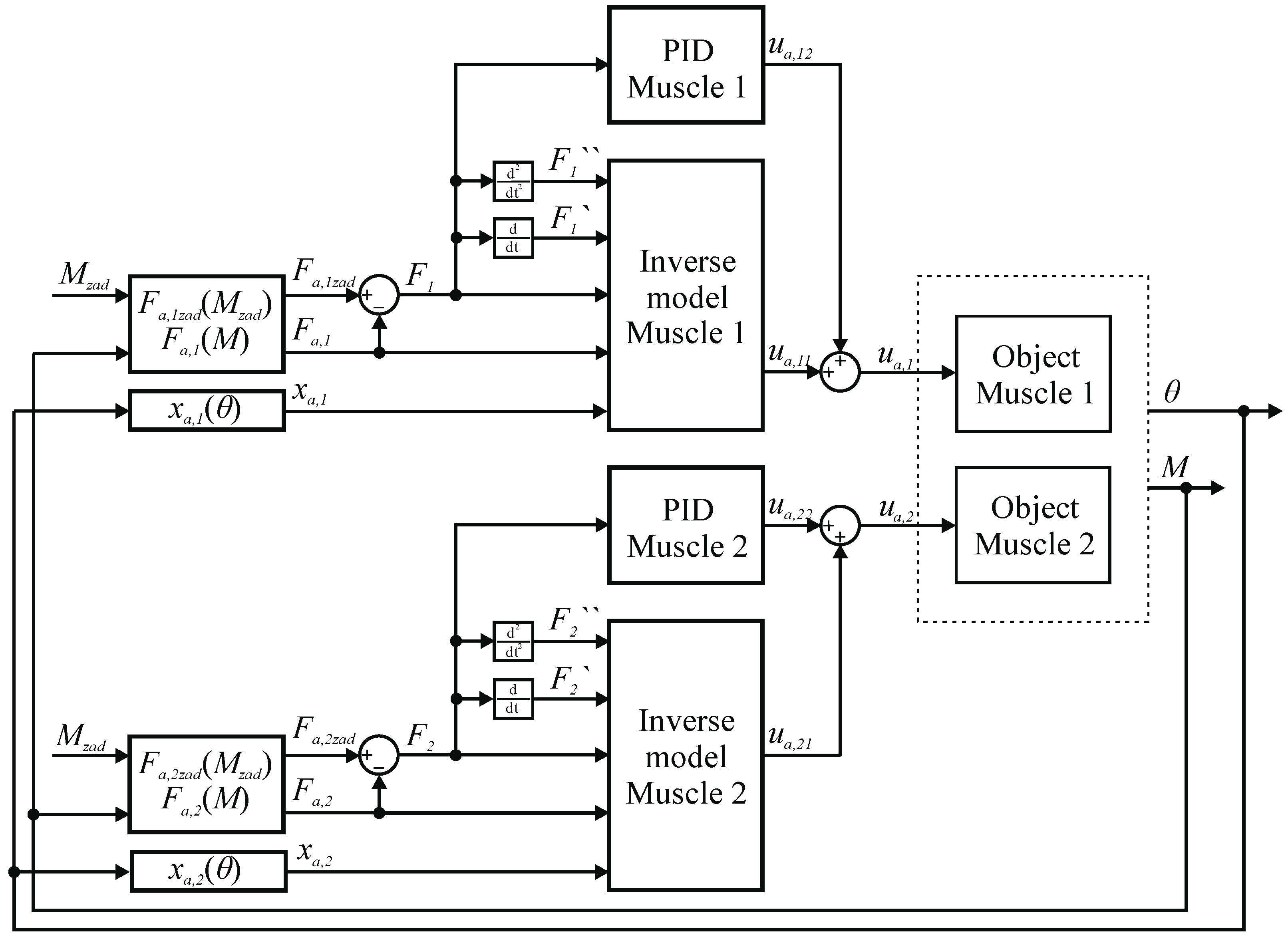
3.2. Synthesis of Regulation System

The servo drive presented in this section is used to work out a given moment of force for a single arm of a parallel manipulator. The locations of all its components are shown in Figure 20.
The servo drive consists of two pneumatic muscles (4). In each of them, one end was immobilized by connecting it to the fixed base (7) through a strain gauge force sensor (6) with a range of ± 2   kN . The free ends of the muscles are connected together by the toothed belt (2) driving the toothed wheel with a pitch diameter of d p = 63.66     mm , thus creating a toothed belt transmission, by means of which the push-pull movement of the muscles is converted into a rotational movement of the arm. The pitch diameter of the pulley and the length of the muscles allow the servo drive to move in the range π 3   rad to π 3   rad , and the maximum force generated by a single muscle allows you to work out a torque of M = 25.46     Nm . The servo drive is also equipped with two pneumatic pressure servo valves (5) controlling the work of the muscles and an absolute angular position sensor (1) with a resolution of 16 bits per revolution, allowing for measuring the angular position with θ   =   9.58 · 10 5   rad accuracy. The diagram also shows an electric servo drive (3), which was used on the test stand to load the muscle servo drive with a given moment of force.
The control system for the torque servo drive has been synthesized. In Figure 21 a diagram of the control system for the entire servo drive is shown, where: θ —current value of the angular position of the servo drive, x a , 1 —current value of the linear position of the first muscle, x a , 2 —current value of the linear position of the second muscle, M —current value of the moment of force generated by the servo drive, F a , 1 —current value of the force generated by the first muscle, F a , 2 —current value of the force generated by the second muscle, M z a d —set value of the moment of force that the servo drive is to generate, F a , 1 z a d —set value of the first muscle strength, F a , 2 z a d —set value of the second muscle strength, F 1 —adjustment error for the first muscle regulator, F 2 —adjustment error for the second muscle regulator, u a , 11 —component of the signal controlling the first muscle valve generated by the inverse model, u a , 12 —signal component controlling the first muscle valve generated by the PIDn controller, u a , 1 —signal controlling the first muscle valve, u a , 21 —signal component controlling the second muscle valve generated by the inverse model, u a , 22 —the component of the signal controlling the second muscle valve generated by the PIDn controller, u a , 2 —signal controlling the second muscle valve.
The servo drive control system consists of two independently operating regulating systems, one for each muscle, in which the controlled quantities are the forces generated by the muscles. The signal about the set point value of the servo drive force is converted into the set value of the first muscle force and is entered into the inverse model of the first muscle. In addition, the signal about the current value of the servo drive torque is converted to the current value of the force generated by the first muscle and is introduced into its inverse model. Furthermore, the signal with the current value of the angular position of the servo drive is converted to the current value of the linear position of the first muscle and is entered into its inverse model. Then, the inverse model of the first muscle generates a control signal. Differences between the set point and the actual value of the force generated by the first muscle, resulting from the inaccuracy of the model, are compensated by the PIDn controller. The control signal generated by the controller is added to the signal generated by the inverse model, and the sum of the signals using the D/A converter is fed to the control valve of the first muscle. The PIDn controller settings were manually selected during tests of the servo drive on the test bench. An analogous method of operation was used for the second muscle regulation system.
In Figure 22, Figure 23, Figure 24, Figure 25 and Figure 26, the results of tests of the developed servo drive maintaining the set moment of force are presented. On the left, the set point waveform is shown in red and the actual value waveform is shown in green. On the right, the error of the servo drive is shown in blue. In Figure 22, the servo drive response to a given sinusoidal signal described by the relationship is shown M   =   5   sin t at an angular position θ   =   0   rad . However, in Figure 23, the servo drive response to a given sinusoidal signal described by the relationship is shown M   =   5   sin ( 3 t ) at an angular position θ   =   0   rad .
In Figure 24 the servo drive response to a given sinusoidal signal described by the relationship is shown M   =   5   sin t 5 at an angular position θ   = π / 9   rad . However, in Figure 25 the servo drive response to a given sinusoidal signal described by the relationship is shown M   =   5   sin ( 3 t ) 5 at an angular position θ   = π / 9   rad .
In Figure 26, the servo drive response to a given rectangular signal with amplitude is shown A   =   5   Nm , period T   =   3   sek and angular position θ   =   0   rad .

4. Conclusions

This article presents the process of designing and building a servo drive consisting of two artificial pneumatic muscles working in opposite directions. The above servo drive is used to generate a given torque of force and is applicable to a parallel manipulator with six degrees of freedom. The mentioned manipulator will be described in more detail in the future. Firstly, we present the construction of the test stand used to determine the characteristics of pneumatic muscles and to test the said servo drive. The methodology of determining families of static characteristics (isobaric, isotonic and isometric) and dynamic characteristics in the form of an object’s response to a step change in the value of the control signal is presented. Then, the method of modeling the behavior of the pneumatic muscle through parametric identification is presented. For each step response, the solution of a second-order differential equation with constant coefficients was fitted, and then the individual coefficients were approximated by a polynomial. In this way, a mathematical model was obtained in the form of a solution of a second-order differential equation with coefficients being polynomials of two variables, and an inverse model in the form of a second-order differential equation with coefficients being polynomials of two variables. Then, the synthesis of the control system for the said servo drive is presented. The system consists of two smaller systems, one for each muscle. Each muscle is controlled by its own inverse model. However, due to the imperfections of the model, an additional PID controller was used. The value of the current strength of each muscle, and thus the current moment of force generated by the servo drive, is read from two strain-gauge force sensors.
The presented mathematical model allows for broad analysis of the behavior of the pneumatic muscle. Due to the use of approximation methods in creating the model, it correctly maps muscle behavior only in terms of displacement and force changes determined in the presented static and dynamic characteristics. The presented comparison of results shows that the model reflects the behavior of the muscle at sinusoidal trajectories very well. However, in the case of abrupt changes in the control signal, a significant deterioration in mapping is noticeable. Analyzing the presented test results of the developed servomotor of the moment of force, it can be seen that the maximum error occurs when the derivative of the set signal is changed. This is probably the result of friction between the braiding fibers of the muscle and between the braiding fibers and the rubber bladder. The influence of friction forces on positioning accuracy is greatest at the rate of change of the set signal close to zero. It was also noted that for low-frequency signals, apart from the moment of changing the derivative sign of the set signal, the error value changes slightly and is not dependent on the current position of the drive. There was also no strong relationship between the accuracy of the servo drive and its angular position. This is evidenced by the fact that the average error values for signals with the same pulsations are similar. Furthermore, the average values of the error module for signals with the same pulsations do not differ from each other. Despite the above negative features of the pneumatic muscle, the developed servo drive is characterized by a relatively good accuracy of work, which allows it to be analyzed as a drive for parallel manipulators. In addition, its unique features, such as high overload capacity, may be highly beneficial in some applications.

Author Contributions

Conceptualization, D.S.P. and P.A.L.; methodology, D.S.P.; software, D.S.P.; validation, D.S.P. and P.A.L.; formal analysis, D.S.P. and P.A.L.; writing—original draft preparation, D.S.P.; writing—review and editing, P.A.L.; supervision, P.A.L. All authors have read and agreed to the published version of the manuscript.

Funding

This research received no external funding.

Institutional Review Board Statement

Not applicable.

Informed Consent Statement

Not applicable.

Data Availability Statement

Not applicable.

Acknowledgments

The authors would like to thank Parker for donating 10 Hoerbiger Tecno Plus valves.

Conflicts of Interest

The authors declare no conflict of interest.

References

  1. Nazarczuk, K. Niektóre Zagadnienia Analizy i Syntezy Sztucznego Mięśnia Pneumatycznego; Archiwum Budowy Maszyn: Warszawa, Poland, 1967. [Google Scholar]
  2. Chou, C.P.; Hannaford, B. Static and Dynamic Characteristics of Mckibben Pneumatic Artificial Muscles. In Proceedings of the 1994 IEEE International Conference on Robotics and Automation, San Diego, CA, USA, 8–13 May 1994; Volume 1–4, pp. 281–286. [Google Scholar] [CrossRef]
  3. Chou, C.P.; Hannaford, B. Measurement and modeling of McKibben pneumatic artificial muscles. IEEE Trans. Robot. Autom. 1996, 12, 90–102. [Google Scholar] [CrossRef] [Green Version]
  4. Doumit, M.; Fahim, A.; Munro, M. Analytical Modeling and Experimental Validation of the Braided Pneumatic Muscle. IEEE Trans. Robot. 2009, 25, 1282–1291. [Google Scholar] [CrossRef]
  5. Takosoglu, J.E.; Laski, P.A.; Blasiak, S.; Bracha, G.; Pietrala, D. Determining the Static Characteristics of Pneumatic Muscles. Meas. Control 2016, 49, 62–71. [Google Scholar] [CrossRef]
  6. Lopez, B.T.i.P. Modeling and control of McKibben artificial muscle robot actuators. IEEE Control. Syst. Mag. 2000, 20, 15–38. [Google Scholar] [CrossRef]
  7. Pietrala, D. The characteristics of a pneumatic muscle. In Proceedings of the EPJ Web of Conferences, online, 4 August 2017; Volume 143, p. 02093. [Google Scholar] [CrossRef] [Green Version]
  8. Pietrala, D.S. Analiza I Synteza Pneumatycznego Serwonapędu Mięśniowego w Zastosowaniu do Manipulatora Równoległego o Sześciu Stopniach Swobody; Rozprawa Doktorska, Politechnika Świętokrzyska: Kielce, Poland, 2020. [Google Scholar]
  9. Carvalho, A.D.D.R.; Karanth, P.N.; Desai, V. Characterization of pneumatic muscle actuators and their implementation on an elbow exoskeleton with a novel hinge design. Sens. Actuators Rep. 2022, 4, 100109. [Google Scholar] [CrossRef]
  10. Dyrr, F.; Dvorak, L.; Fojtasek, K.; Brzezina, P.; Hruzik, L.; Burecek, A. Experimental analysis of fluidic muscles. MM Sci. J. 2022, 2022, 5759–5763. [Google Scholar] [CrossRef]
  11. Xavier, M.S.; Tawk, C.D.; Zolfagharian, A.; Pinskier, J.; Howard, D.; Young, T.; Lai, J.; Harrison, S.M.; Yong, Y.K.; Bodaghi, M.; et al. Soft Pneumatic Actuators: A Review of Design, Fabrication, Modeling, Sensing, Control and Applications. IEEE Access 2022, 10, 59442–59485. [Google Scholar] [CrossRef]
  12. Kalita, B.; Leonessa, A.; Dwivedy, S.K. A Review on the Development of Pneumatic Artificial Muscle Actuators: Force Model and Application. Actuators 2022, 11, 10. [Google Scholar] [CrossRef]
  13. Ganguly, S.; Garg, A.; Pasricha, A.; Dwivedy, S.K. Control of pneumatic artificial muscle system through experimental modelling. Mechatronics 2012, 22, 1135–1147. [Google Scholar] [CrossRef]
  14. Godage, I.S.; Branson, D.T.; Guglielmino, E.; Caldwell, D.G. Pneumatic Muscle Actuated Continuum Arms: Modelling and Experimental Assessment. In Proceedings of the 2012 IEEE International Conference on Robotics and Automation (ICRA), Saint Paul, MN, USA, 14–18 May 2012; pp. 4980–4985. [Google Scholar]
  15. Kang, B.-S.; Kothera, C.S.; Woods, B.K.S.; Wereley, N.M. Dynamic Modeling of Mckibben Pneumatic Artificial Muscles for Antagonistic Actuation. In Proceedings of the ICRA: 2009 IEEE International Conference on Robotics and Automation, Kobe, Japan, 17 May 2009; Volume 1–7, p. 643+. [Google Scholar]
  16. Shen, X. Nonlinear model-based control of pneumatic artificial muscle servo systems. Control Eng. Pract. 2010, 18, 311–317. [Google Scholar] [CrossRef]
  17. Zhang, D.; Zhao, X.; Han, J. Active Model-Based Control for Pneumatic Artificial Muscle. IEEE Trans. Ind. Electron. 2017, 64, 1686–1695. [Google Scholar] [CrossRef]
  18. Dai, Z.; Rao, J.; Xu, Z.; Lei, J. Design and Joint Position Control of Bionic Jumping Leg Driven by Pneumatic Artificial Muscles. Micromachines 2022, 13, 6. [Google Scholar] [CrossRef] [PubMed]
  19. Andrikopoulos, G.; Nikolakopoulos, G.; Manesis, S. Advanced Nonlinear PID-Based Antagonistic Control for Pneumatic Muscle Actuators. IEEE Trans. Ind. Electron. 2014, 61, 6926–6937. [Google Scholar] [CrossRef]
  20. Minh, T.V.; Tjahjowidodo, T.; Ramon, H.; Brussel, H.V. Control of a Pneumatic Artificial Muscle (PAM) with Model-Based Hysteresis Compensation. In Proceedings of the 2009 IEEE/ASME International Conference on Advanced Intelligent Mechatronics, Suntec Convention and Exhibition Center, Singapore, 14–17 July 2009; Volume 1–3, p. 1086+. [Google Scholar] [CrossRef]
  21. Minh, T.V.; Tjahjowidodo, T.; Ramon, H.; Brussel, H.V. Cascade position control of a single pneumatic artificial muscle-mass system with hysteresis compensation. Mechatronics 2010, 20, 402–414. [Google Scholar] [CrossRef]
  22. Minh, T.V.; Kamers, B.; Tjahjowidodo, T.; Ramon, H.; Brussel, H.V. Modeling Torque-Angle Hysteresis in a Pneumatic Muscle Manipulator. In Proceedings of the 2010 IEEE/ASME International Conference on Advanced Intelligent Mechatronics (AIM), Montreal, QC, Canada, 6–9 July 2010. [Google Scholar] [CrossRef]
  23. Minh, T.V.; Kamers, B.; Ramon, H.; Brussel, H.V. Modeling and control of a pneumatic artificial muscle manipulator joint—Part I: Modeling of a pneumatic artificial muscle manipulator joint with accounting for creep effect. Mechatronics 2012, 22, 923–933. [Google Scholar] [CrossRef]
  24. Yeh, T.-J.; Wu, M.-J.; Lu, T.-J.; Wu, F.-K.; Huang, C.-R. Control of McKibben pneumatic muscles for a power-assist, lower-limb orthosis. Mechatronics 2010, 20, 686–697. [Google Scholar] [CrossRef]
  25. Qin, Y.; Zhang, H.; Wang, X.; Han, J. Active Model-Based Hysteresis Compensation and Tracking Control of Pneumatic Artificial Muscle. Sensors 2022, 22, 1. [Google Scholar] [CrossRef] [PubMed]
Figure 1. View of the developed pneumatic artificial muscle.
Applsci 12 11024 g001
Figure 2. Methodology for determining static characteristics.
Applsci 12 11024 g002
Figure 3. Model and real view of the test stand. 1—planetary gear, 2—absolute optical encoder, 3—toothed belt, 4—pneumatic muscle, 5—pressure servo valves, 6—force sensor.
Applsci 12 11024 g003
Figure 4. Exemplary isobaric characteristics.
Applsci 12 11024 g004
Figure 5. Surface of isobaric characteristics.
Applsci 12 11024 g005
Figure 6. Hysteresis surface of isobaric characteristics.
Applsci 12 11024 g006
Figure 7. Exemplary isotonic characteristics.
Applsci 12 11024 g007
Figure 8. Surface of isotonic characteristics.
Applsci 12 11024 g008
Figure 9. Hysteresis surface of isotonic characteristics.
Applsci 12 11024 g009
Figure 10. Exemplary isometric characteristics.
Applsci 12 11024 g010
Figure 11. Surface of isometric characteristics.
Applsci 12 11024 g011
Figure 12. Hysteresis surface of isometric characteristics.
Applsci 12 11024 g012
Figure 13. Exemplary dynamic characteristics (step increase in the control signal).
Applsci 12 11024 g013
Figure 14. Exemplary dynamic characteristics (step decrease in the control signal).
Applsci 12 11024 g014
Figure 15. Model matching results at selected work points ( x a = 5   mm ,   x a = 20   mm ,   x a = 35   mm ).
Applsci 12 11024 g015
Figure 16. Model matching results at selected work points ( x a = 50   mm ,   x a = 65   mm ,   x a = 80   mm ).
Applsci 12 11024 g016
Figure 17. Schematic diagram of the control system used to verify the models.
Applsci 12 11024 g017
Figure 18. The results of verification of the model fit for strength (for x a   =   20   mm ).
Applsci 12 11024 g018
Figure 19. The results of verification of the model fit for strength (for x a   =   50   mm ).
Applsci 12 11024 g019
Figure 20. Diagram of a servo drive structure. 1—absolute angular position sensor, 2—toothed belt, 3—electric servo drive, 4—pneumatic muscle, 5—pneumatic pressure servo valves, 6—force sensor, 7—base.
Applsci 12 11024 g020
Figure 21. Diagram of the control system for torque servo drive.
Applsci 12 11024 g021
Figure 22. Torque servo test results for reference signal M   =   5   sin t . Red—command signal, green—measured signal, blue—error.
Applsci 12 11024 g022
Figure 23. Torque servo test results for reference signal M   =   5   sin ( 3 t ) . Red—command signal, green—measured signal, blue—error.
Applsci 12 11024 g023
Figure 24. Torque servo test results for reference signal M   =   5   sin t 5 . Red—command signal, green—measured signal, blue—error.
Applsci 12 11024 g024
Figure 25. Torque servo test results for reference signal M   =   5   sin ( 3 t ) 5 . Red—command signal, green—measured signal, blue—error.
Applsci 12 11024 g025
Figure 26. Torque servo test results for reference signal A   =   5   Nm , T   =   3   sek . Red—command signal, green—measured signal, blue—error.
Applsci 12 11024 g026
Publisher’s Note: MDPI stays neutral with regard to jurisdictional claims in published maps and institutional affiliations.

