Featured Application
Quantitative and calibration free determination of the absolute optical properties of turbid samples in a standard cuvette with milliliter scale volume.
Abstract
Many applications seek to measure a sample’s absorption coefficient spectrum to retrieve the chemical makeup. Many real-world samples are optically turbid, causing scattering confounds which many commercial spectrometers cannot address. Using diffusion theory and considering absorption and reduced scattering coefficients on the order of and 1, respectively, we develop a method which utilizes frequency-domain to measure absolute optical properties of turbid samples in a standard cuvette (). Inspired by the self-calibrating method, which removes instrumental confounds, the method uses measurements of the diffuse complex transmittance at two sets of two different source-detector distances. We find: this works best for highly scattering samples (reduced scattering coefficient above 1 ); higher relative error in the absorption coefficient compared to the reduced scattering coefficient; accuracy is tied to knowledge of the sample’s index of refraction. Noise simulations with % amplitude and phase uncertainty find errors in absorption and reduced scattering coefficients of 4% and 1%, respectively. We expect that higher error in the absorption coefficient can be alleviated with highly scattering samples and that boundary condition confounds may be suppressed by designing a cuvette with high index of refraction. Further work will investigate implementation and reproducibility.
1. Introduction
Samples in which the propagation of light is dominated by random scattering are considered optically diffuse. Such samples can be characterized by two absolute optical properties, the absorption coefficient () and the reduced scattering coefficient () [1]. The represents chemical information, and its spectral measurement allows for determination of the sample’s chemical constituents and concentrations. Meanwhile, the describes the scale structure of diffuse samples. However, in many applications is considered a confounding parameter, since measurement of and chemical makeup is often the end goal. For this reason, even when diffuse sample measurement of only is sought, must also be determined since it significantly impacts the behavior of light and thus the recovered .
Applications that seek to measure these diffuse optical properties are numerous and span many fields. For example, applications include those within biomedical research and clinical applications [1,2,3], of food science and quality [4,5,6], concerning pharmaceutical metrology [7,8], pertaining to art and archaeology [9,10], and within dendrology [11] to name a few. In all cases, one has two options:
- To make a measurement which retrieves the total attenuation coefficient () or the effective attenuation coefficient ().
- To make a measurement that can separate both and .
However, only option 2 allows for careful quantitative analysis of the sample properties; since in option 1 one can only measure a coefficient, namely or , that couples both the and of the sample. There are few methods capable of achieving option 2. One such technique is Near-InfraRed Spectroscopy (NIRS) implemented in Frequency-Domain (FD) [12] (or Time-Domain (TD) [13]) which can recover and by using temporally modulated light. In the case of FD, photon density waves are generated by using a sinusoidally modulated source on the order of 100 , and the amplitude and phase of these photon density waves are measured from the detected modulated light signal. An example of a commercially available FD instrument capable of this measurement is the ISS Imagent V2 [Champaign, IL USA] (Imagent). A second technique capable of option 2 is the integrating sphere [14,15]. This technique measures total diffuse reflectance and total diffuse transmittance to separate and . Both techniques have their strengths and weaknesses. Common implementations of FD NIRS require large sample volumes to create geometries that are effectively infinite in at least one dimensional extent making simple diffusion theory expressions valid [16]. Other methods, besides diffusion theory, exist to tackle non-simple geometries such as Monte Carlo [17] and the radiative transport equation implemented with higher order spherical harmonics [18,19,20]. However these methods are computationally costly compared to diffusion theory and would likely be impractical to implement on a broad range of optical wavelengths (s). Another weakness of FD regarding the number of s, is the typical implementation at only discrete s such as with the Imagent. Meanwhile, the integrating sphere requires careful calibration or a reference sample and is easily susceptible to errors induced by the measurement technique (for example, light loss causing an incorrect measurement of total reflectance and transmittance).
Due to these difficulties with option 2 (and relative ease implementing option 1), most commercial spectrometers make a measurement that is based on the retrieving non-diffuse transmittance. Therefore, for quantitative determination of a sample’s chemical concentrations (through the spectrum), samples must be non-scattering or transparent; either innately or through some chemical washing. Whenever this is not possible the measurement will be confounded by scattered light. This implies that the will be overestimated and its spectral dependence distorted leading to errors in the estimation of a sample’s chemical constituents.
One such instrument that shines when samples are transparent and non-scattering is the Perkin Elmer LAMBDA 365+ (Waltham, MA, USA), this and instruments like it are the workhorses of many chemical and biological laboratories. However, when diffuse sample measurement is necessary (and quantitative measurement of properties sought), one of the aforementioned techniques capable of option 2 is required. One example is the Gigahertz
Optik SphereSpectro 150H (Tüerkenfeld, Germany) (SphereSpectro), an instrument directly designed for spectroscopic measurement of both and via integrating sphere. Furthermore, integrating spheres may be purchased as attachments to traditional spectrometers, thus adding diffuse functionality. One such example of a spectrometer that has this option is the Perkin Elmer LAMBDA 1050+ (Waltham, MA, USA). However, we are not aware of any commercially available instrument that utilizes the FD in such applications.
Because of the apparent gap in the market for instruments which complete diffuse measurement of and , namely implementation with instruments that utilize FD NIRS like techniques, we will focus closer on FD. Measurements of and with temporally modulated light, such as FD NIRS, is actually rather common but typically only in the research setting (using the Imagent for example). However, we know of no FD instruments designed for the sample sizes and form factors of traditional spectrometers which accept a cuvette. In-fact FD NIRS methods typically require large sample volumes on the scale of to implement simple diffusion theory solutions. Two examples of work that considered FD measurements in confined regions were that in the slab [21] or block [22] (which utilized the same diffusion theory model implemented here [23]), however the geometries considered in these works were rather large compared to a cuvette. There are advantages of FD NIRS which would lead one to seek or design and manufacture such an instrument. For example, FD NIRS can leverage existing techniques which eliminate the need for instrumental calibration such as the Self-Calibrating (SC) method [24]. Additionally, despite FD typically being implemented at discrete , methods exist to achieve broadband measurement. This may be done by combining measurements at discrete s in FD (or TD) with measurements at broadband s with Continuous-Wave (CW) [25,26,27], implemented with SC and a method dubbed Dual-Slope (DS), respectively, [28,29,30]. This leverages the fact that SC and DS both rely on a difference type measurement which is capable of subtracting away instrumental confounds.
We see an opportunity to develop a method which leverages the tools available in FD NIRS to measure absolute and in a standard cuvette with scale volume in an attempt to compete with the existing integrating sphere type devices. Therefore, in this work we present a method that utilizes FD NIRS in a small geometry the size of a standard cuvette ( ). Our proposal relies on the SC/DS method to remove a majority of the instrumental confounds. To our knowledge no work has yet leveraged SC/DS directly on the cuvette geometry as we propose here. First, we utilize a seldom implemented but still computationally inexpensive diffusion theory derived expression for the box geometry [23] to model our proposed measurement and determine the method’s feasibility in theory. Then we further develop ways to retrieve and from the proposed measurement. Lastly, we determine the strengths and weaknesses of the proposed method. Our end goal is to implement the method for broadband measurement of [28], thus computation cost and model simplicity are of importance leading to the choice of a diffusion theory model. In this article we focus only on the FD part since the extension to broadband CW will utilize all the same theory.
2. Methods
2.1. Geometry
In this work, we consider a box geometry with the dimensions of a standard cuvette ( ; Figure 1). A DS/SC arrangement (the word slope in Dual-Slope (DS) is historical [29,30] as no slopes are actually considered in this work) is achieved by placing 2 sources (1 & 2; Figure 1a,b) and 2 detectors (A & B; Figure 1b,c) symmetrically on opposing sides of the cuvette. Using the coordinate system shown in Figure 1, the optodes were considered at the following position vectors (s): , , , and . This forms two possible source-detector distances (s) of 14.9 mm and 25.1 (2 each), for 1A & 2B and 2A & 1B, respectively.
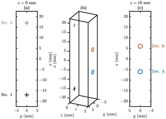
Figure 1.
Schematic diagram of cuvette geometry measuring . Sources and detectors are considered at the following s: , , , and . (a) plane for . (b) Transparent projected view. (c) plane for . Acronyms and Symbols: Position vector ().
2.2. Types of Measurement
The signal obtained between a single temporally modulated source and a single detector recovers the Green’s function for the complex Transmittance with FD NIRS. is a complex number to represent the amplitude and phase of the transmitted photon density waves modulated on the order of 100 . These signals are named: , , , and ; where the first subscript indicates the source and the second the detector. The short measurements () are and while the long measurements () are and .
From these measurements, ratios between the short and long measurements may be obtained. Therefore we introduce the Single-Ratio of the s for the geometry in Figure 1 as follows:
and the Dual-Ratio of the as the geometric mean of the two symmetric s.
This forms a similar type of measurement to DS/SC but replacing the concept of slope with that of ratio (The word slope in Dual-Slope (DS) is historical [29,30] as no slopes are actually considered in this work). We acknowledge that the notation used here is verbose since, that even for we utilize subscripts to show all optodes used. However, for this work we have opted to use this notation to distinguish explicitly, the origin of the measurements. This is helpful in observing the differences in s, particularly in Section 3.1.2. In other work we opt to utilize a simpler notation with numbered subscripts [30].
We can further expand the expression for to consider amplitude () and phase (). For example, with 1AB we have:
and we introduce the final ratio type, the natural logarithm of :
The motivation for utilizing the natural logarithm in this way is that it partly linearizes typical expressions for diffuse optical measurements ( in this case) as a function of [31]. Additionally it shows a symmetry between and as they are both differences. This work focuses on utilizing these and ratio types in the development of the proposed method.
Note that similar expressions can also be written for , amplitude phase (), and natural logarithm of ():
From this it can be seen that is a geometric mean of s and both as well as are arithmetic means of s and s, respectively.
For theoretical calculations, not considering optode coupling differences and medium heterogeneity, the different s and s have the same value. This is due to the symmetry shown in Figure 1 considering a homogeneous medium. For this reason, only the set 1AB, and , is considered for most of the results. Coupling is considered in Section 3.1.2, therefore, discrepancies between the difference measurements are investigated in that section and the distinction between and becomes important there.
2.3. Analytical Box Model
To generate data for the cuvette geometry (Figure 1) we utilized the following diffusion theory derived analytical expression for the [23] (The expression used for the Green’s function for the complex Transmittance () represents the measured transmittance normalized by the source power giving it units of mm−2):
where the optical properties, the and the , are contained within the complex effective attenuation coefficient ():
and the remaining non-spatial variables are the angular modulation frequency (), the index of refraction (n) inside the medium (), and the speed of light in vacuum (c).
For spatial variables we first have the cuvette dimensions: , , and (Figure 1). Next, we have the source coordinates: and (given that a pencil beam impinges on the face so that an isotropic source is placed at ); as well as the detector coordinates: and (given that the detector is placed on the face, thus ). Using these variables and remembering the sum indexes from Equation (10) we can now write the various point source positions (infinite of both positive and negative as per the indexing variables l, m, and n) [23]:
where h is the distance between the extrapolated boundary and the actual box boundary:
a is the n mismatch parameter [16,32] which is a function of the relative n mismatch (, where is the n outside). Finally, using these positions, we can define the distances to the point sources:
This diffusion theory derived expression (Equation (10)) was previously presented and validated against Monte Carlo in [23]. The validity of such an expression is dependent on the distance from the source, the value of , and the ratio between and . Only locations far enough from the source for scattering to be considered isotropic may be considered, must be large enough for isotropic scattering to dominate within the medium, and must be much less than . Given that we consider measurements on the opposite side of a 10 thick cuvette the first and second conditions are met for values on the order of 1 (cuvette thickness of 10 isotropic scattering mean free paths). Finally, the last condition may be met by considering values of on the order of 100 times smaller than . For this work, we choose values which encompass the edge of validity of diffusion theory with from 0 –0.05 and from 0.5 –5 for demonstration purposes. Most focus is on the values of for and 1 for , for which our independent (aside from what is presented in [23]) validation against Monte Carlo [17] found % discrepancy for and for over the face of the cuvette opposing the source. For the purposes of this work, a feasibility study of the proposed method, we believe this diffusion theory model is appropriate.
To provide some physical intuition regarding the FD portion of this model, we can discuss the wavelength of the photon density waves (), which can be approximated as [1]:
This leads to a of about 160 using values of for , 1 for , for , 1 for n, and for c. This is larger then the cuvette, but not so large that it dwarfs the cuvette scale completely. This indicates that phase measurements are reasonable for this volume, given that the phase will not wrap ( not too short) but will still change considerably throughout the size of the cuvette ( not too long).
To demonstrate the implementation of this expression for (Equation (10)) we show a map of the amplitude () and phase () on the face (opposing the source; Figure 1) for and in Figure 2 (considering source 1). This shows the spatial continuum of which can be simulated with diffusion theory. The positions of the source (1) and detectors (A & B) are also indicated in Figure 2 to show the positions which will be considered throughout this work. For computation based on Equation (10), l, m, and n were each summed from -3 to 3, and inclusion of more terms was found to not significantly impact the results.
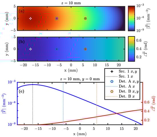
Figure 2.
Example of the implementation of the diffusion theory derived expression for in Equation (10) showing (The expression used for the Green’s function for the complex Transmittance () represents the measured transmittance normalized by the source power giving it units of ) on the cuvette face opposing the source () considering the geometry in Figure 1 and source 1. For this simulation the was , the 1 , n inside 1.3, n outside 1, , and the cuvette measured . The source ( position is shown as cross; x position as black dotted line) was placed at . Detector positions which are considered in the following work are shown as circles (for position) or dotted lines (for x position) (a) amplitude () on the plane at . (b) phase () on the plane at . (c) and along the x direction for and . Acronyms and Symbols: Green’s function for the complex Transmittance (), absorption coefficient (), reduced scattering coefficient (), index of refraction (n), angular modulation frequency (), and position vector ().
2.4. Optical Properties Fit
The end goal of this work is to develop a method capable of measuring the absolute and in the geometry of Figure 1 using FD. With this in mind, we define a cost () function which can be minimized by varying and , thus creating a fit for and (We acknowledge that the cost () function is dependent on parameters beyond absorption coefficient () and reduced scattering coefficient () such as index of refraction (n), and investigate this in further sections of this work):
where the subscript represents the measured difference (In this work, the measurement is simulated using Equation (10), and noise may be added depending on the purpose) and the subscript represents the value retrieved from Equation (10) considering a particular and (Again we note that the Dual-Ratio of the () and a Single-Ratio of the () are the same when not considering optode coupling (shown in Section 3.1.2)).
Three further variables are introduced in Equation (28), which we define below. First is the scaling coefficient () which is discussed further in Section 3.2.1. Second and third are the uncertainties of () and () which are expressed based on 1st order error propagation as:
and
where, is the uncertainty in and is the uncertainty in , and assuming that the uncertainties in the two s () and the two s () are each the same. For this work we set and which would be typical for a FD NIRS instrument such as the Imagent.
3. Results
3.1. Investigation of Difference Measurements
3.1.1. Variation over Optical Properties
The chief measurements which we consider are and (or and considering coupling; (Again we note that the Dual-Ratio of the () and a Single-Ratio of the ) () are the same when not considering optode coupling (shown in Section 3.1.2))). Figure 3 shows these measurements (Equations (5) and (6)) over a large range of optical properties, specifically and (Figure 3a,c) or and (Figure 3b,d).
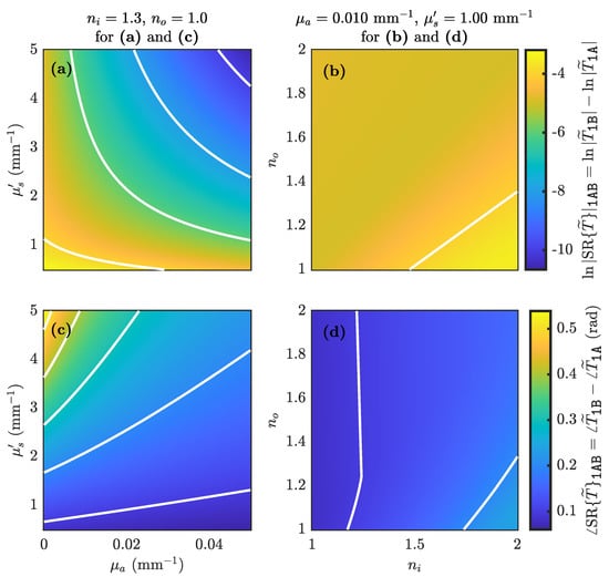
Figure 3.
How the measurements of the and (Equations (6) and (5)) are effected by optical parameters, namely the , the , the n inside () and the n outside (). Simulation geometry and parameters not explicitly shown here are stated in detail in Figure 1 and Figure 2. (a) versus and . (b) versus and . (c) versus and . (d) versus and . Note: (a,b) have the same iso-line and color-map values/scales; as do (c,d). Acronyms and Symbols: Green’s function for the complex Transmittance (), Single-Ratio of the Green’s function for the complex Transmittance () (), amplitude (), natural logarithm of (), phase (), absorption coefficient (), reduced scattering coefficient (), and index of refraction (n).
Since the intention is to convert these measurements of and to and , the desire is for the measurements to vary significantly more as and are varied as compared to varying and . The iso-lines (white lines) in Figure 3a,b consider the same values (the same is true for Figure 3c,d). From this we see that varying and varies across 4 more iso-lines than varying and (and about 2 times more for ). This suggests promise in the goal of retrieving and .
To recover and from and we must also have significantly different information in and so that the recovered variables ( and ) have a unique solution and little cross-talk. There is also promise along these lines as the iso-lines in Figure 3a versus Figure 3c are qualitatively orthogonal. This suggests a fit to and from and should be possible. This is further investigated in Section 3.2.
One final insight that can be drawn from Figure 3 is the effect of which is constant along diagonal lines with positive slopes in Figure 3b,d. From this we see that is little effected by . Further, in the upper left portion of the plots where is only significantly effected by . Therefore we may be able to optimize the design of the cuvette boundary to reduce cross-talk with the ns which is discussed further in Section 4.
3.1.2. Optode Coupling and Auto-Calibration
As has been stated above including in (Again we note that the Dual-Ratio of the () and a Single-Ratio of the () are the same when not considering optode coupling (shown in Section 3.1.2)), & (as well as & , & , and & ) are equivalent when optode coupling is not considered. For this reason, other sections of this manuscript are not careful to distinguish between them as theoretical calculations are being carried out and coupling is not a consideration. However, in this section we show the effect of optode coupling and the auto-calibration of the which is inherited/inspired by the SC method [24].
To do this, first we define a complex optical Coupling, power, and/or efficiency factor () for each optode: , , , and . Physically, represents a multiplicative factor (attenuation or amplification) on the amplitude of and represents a phase shift on the phase of . s applied to sources (number subscripts) have units of since their amplitude also includes source power; while s for detectors (letter subscripts) are unit-less. Therefore, adding subscripts to our measurements when they are confounded by coupling (opposed to the theoretical value without the subscript) we have the following signals considering coupling:
Now, let us revisit Equations (1)–(3) but with optode coupling considered:
showing that the measured is the same as the theoretical values regardless of the various optode couplings . Notice that the same follows for , , and .
This property of auto-calibration (coming from the SC method [24]) is demonstrated in Figure 4. However, in this case, unlike SC, the symmetry requirements are not as strict since ratios instead of slopes are used as the measurement. In this case a random was applied for each optode and the difference measurements both averaged and not were simulated. From Figure 4 one can see that the and measurements are the same as the theoretical values. This is significant since it shows that the proposed measurement method would be insensitive to optode coupling, and further, optode coupling would not effect the recovered and . Therefore, the instrument would not need to be calibrated in terms of coupling, reducing possible systematic errors and making the method simpler to implement.
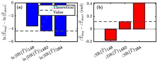
Figure 4.
Demonstration of the cancellation of coupling factors when considering the and measurements. For this simulation, random s were generated for each optode and Equations (33)–(36) implemented. All other simulation parameters are the same as Figure 1 and Figure 2. The expected theoretical value for the measured differences is shown as a dashed line. (a) The two symmetric measurements and the measurement. (b) The two symmetric measurements and the measurement. Acronyms and Symbols: Green’s function for the complex Transmittance (), Single-Ratio of the (), amplitude (), natural logarithm of (), phase (), Dual-Ratio of the (), amplitude (), natural logarithm of (), phase (), and complex optical Coupling, power, and/or efficiency factor ().
3.2. Development of Fit for Absolute Optical Properties
3.2.1. Optimization of Cost Space Shape
In order to fit for the absolute optical properties and we consider the function in Equation (28). This function contains the scaling parameter which balances the scale of versus . The intention of such a parameter is to modify the space to be as circular as possible. This circularity can be quantitatively defined by considering iso-lines in cost space and their perimeter (P) as well as area (A). A circle has the minimum ratio of P to A of all 2-Dimensional (2D) shapes. Therefore, the dimensionless metric was minimized by varying (note that has a minimum theoretical value of , for a circle) [33].
The effect of the value on space shape is shown in Figure 5 using the same parameters as Figure 1 and Figure 2 (where the optical properties are the values). Figure 5b shows the optimal of 1.2 × 10⁻³, which is the case where was minimized. The resulting , for this optimal was 36 about 3 times worse than the value of for a ideal circular cost space. This can be seen by how oblique the iso-lines are in the direction suggesting a higher relative uncertainty in . We investigate this further in Section 3.3. Figure 5a,c show the effect of favoring either the or term in the expression (Equation (28)). In either case and are correlated and the space is spread more in . However, when is favored (Figure 5c) and have a negative correlation while the correlation is positive when is favored (Figure 5a).
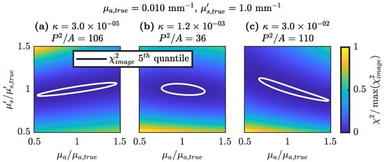
Figure 5.
Three examples of the (Equation (28)) space shape for different s. The shape of cost space is determined by the shape of an iso-line and its ratio of P squared divided by A () which has a minimum possible value of (in the case of a circle). Iso-lines are the 5th quantile of all values in each image and are meant to represent the overall shape of space. For all axes, , the , and the are normalized. (a) and . (b) Optimal value of for the optical properties used here found by minimizing , resulting in and . (c) and . Acronyms and Symbols: Cost (), scaling factor (), Perimeter (P), Area (A), absorption coefficient (), and reduced scattering coefficient ().
Note that the optimal was found for the of and of 1 and a different optimal s may be found elsewhere for different and . Despite this we have opted to utilize this one value for the rest of this work to reduce computation time, in the future a map of optimal could be found as a function of and .
3.2.2. Cost Space Shape for Various Optical Properties
Now that the entire cost (; Equation (28)) function including has been determined, we can plot some example cost spaces for various s and s. This is shown for 9 cases in Figure 6. For the 9 cases all combinations of the following optical properties were used: 0.005 , 0.010 and 0.020 combined with 0.5 , 1.0 and 2.0 .
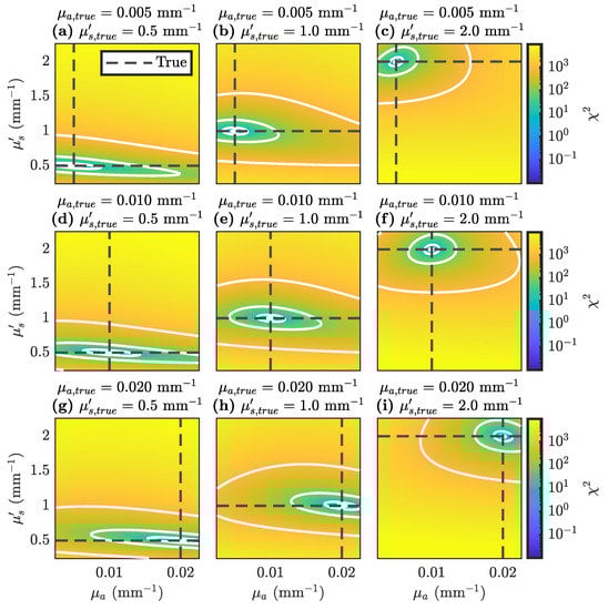
Figure 6.
9 examples of (Equation (28); ) space for different sets of the and . (a) and . (b) and . (c) and . (d) and . (e) and . (f) and . (g) and . (h) and . (i) and . Acronyms and Symbols: Cost (), scaling factor (), absorption coefficient (), and reduced scattering coefficient ().
Examining Figure 6 we notice that in general will likely have more error or has a less unique solution compared to . This is evident by the spreading of the low values of along the direction near the local minimum and value. This result is an extension of what was seen for one set of optical properties in Figure 5b. We also notice that this oblique space shape is worse for small ( ), which is somewhat expected since diffusion theory is not meant to be used in the low scattering regime. For this reason, finding optimal as a function of and may help alleviate this problem. Regardless, from this result we should expect the fit to work less well when attempting to retrieve when is low.
3.2.3. Fit Initial Guess
We finish our development of the fit for and with a demonstration of exact retrieval when the same inverse and forward models are used for without noise (Equation (10)). In doing so we also investigate the effect of different initial guesses on and to show that convergence is not dependent on this initial guess (The result is not dependent of initial guess given that the initial guess is of reasonable optical properties). For this, the fit was implemented by using the MathWorks MATrix LABoratory [Natick, MA USA] (MATLAB) function fmincon to minimize (Equation (28); ) function. For fmincon, the algorithm interior-point was used and the minimum constraints on and set to [0,0], respectively, with all other bound types unconstrained.
Using this optimization setup, the fit was run with the and the using 4 different initial es:
- & .
- & .
- & .
- & .
The results from these fits and the fit trajectory (shown as dotted lines with circles) are shown in Figure 7. In all cases the fit converged to the optical properties regardless of start point. A second observation that can be made from Figure 7 is what trajectory the fit follows during convergence. Acknowledging that this is highly dependent on algorithm choice, we still note that the fit spent most of its time traversing in the direction, converging close to the correct comparatively fast. This is a consequence of the shape of cost space, having a longer trough in the direction than the .
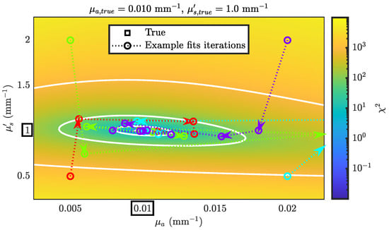
Figure 7.
Example trajectories of fmincon minimization of (Equation (28); ) to fit for the and the . Results from 4 different initial es shown: (Red) & . (Green) & . (Cyan) & . (Purple) & . Acronyms and Symbols: Cost (), scaling factor (), absorption coefficient (), and reduced scattering coefficient ().
3.3. Confounds to Fit Retrieved Absolute Optical Properties
3.3.1. Propagation of Noise to Optical Property Uncertainty
To test how noise propagates through the recovery of and , when using the fit developed in Section 3.2, we simulated and as mentioned in Section 2.4. This was done by simulating measured and 101 times and each time adding Gaussian noise with the s stated above. For each of the 101, the fit was run to recover some and . This was done for all 9 of the sets of and shown in Figure 6.
The results from this exercise are shown in Figure 8 and Table 1, from these three main observations can be drawn:
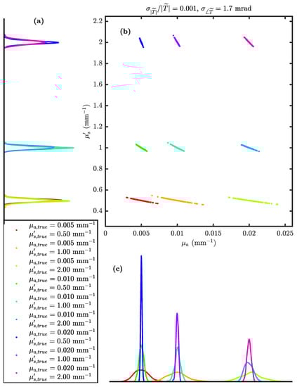
Figure 8.
Result from 101 simulations of noise ( and ) for the 9 different sets of the and the shown in Figure 6. (a) Marginal histograms for recovered values of the 9 sets of optical properties and 101 noise simulations. (b) Scatter plot of recovered and for the 9 × 101 noise simulations. (c) Marginal histograms for recovered values of the 9 sets of optical properties and 101 noise simulations. Acronyms and Symbols: Green’s function for the complex Transmittance (), uncertainty (), absorption coefficient (), and reduced scattering coefficient ().

Table 1.
Errors for 9 sets of optical properties and 101 noise simulations using and .
- The fractional error in is always larger compared to suggesting the system can more precisely recover .
- Errors in are much larger for small and slightly larger for small (with small and together being the worst case).
- That and are highly negatively correlated (as suggested by Figure 5b,c).
Observation A again expounds upon what has been expected from the shape of space presented in previous sections. Furthermore, observations B and C are typical for such diffusion theory based problems.
To draw some quantitative values for this exercise, we can closely examine Table 1. It is helpful to extract the worst case (for the type of simulations we have done), and typical (considering typical being the case when and ) fractional errors in and . These are as follows:
- For :
- –
- Typical error of 4%.
- –
- Worst case error of 20% (for low and ).
- For :
- –
- Typical error of 1%.
- –
- Worst case error of 3% (for high and low ).
Of course these values are dependent on the simulated measurement errors of and which may be different for different instruments.
3.3.2. Assumption of Index of Refraction
Finally, we examine how the assumption of n (and by extension the model boundary conditions) affects the recovered and . We have done this by running the fit ing sets of and , but generating forward data with different ns in the range 1 to 2 (we do not co-vary and for simplicity). 2 sets of ns in the fit were invested:
- & (Figure 9 solid lines).
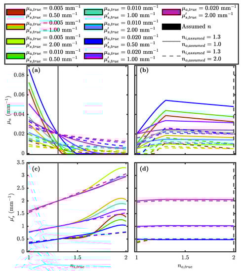 Figure 9. Effect of recovered and on the n inside () and outside () when fixed values of ns are . Shown for the 9 sets of optical properties used in Figure 6. (Solid Lines) and in fit. (Dashed Lines) and in fit. (a) Recovered while varying and fixing to the value. (b) Recovered while varying and fixing to the value. (c) Recovered while varying and fixing to the value. (d) Recovered while varying and fixing to the value. Acronyms and Symbols: absorption coefficient (), reduced scattering coefficient (), and index of refraction (n).
 - & (Figure 9 dashed lines).
This exercise was done for all 9 sets of and shown in Figure 6.
Figure 9 shows these recovered and for the 2 cases while varying and . First, we note that has a larger effect on the recovered and compared to , with having a negative, and a positive, correlation with (Figure 9a,c). Furthermore, is much more strongly affected by than , with recovered values being up to about 7 times greater than the value when there is a low value. For high the recovered often approaches 0 (hitting the fmincon constraint). All of this suggests that the method’s ability to accurately recover and particularly is dependent on knowledge of .
Now, focusing on Figure 9b,d, we see the effect of . In this case is almost not affected at all by and is much more significantly affected when or . In this case the correlation between and is positive (opposite to that for ), suggesting a connection to the dependence on . These results further re-enforce the idea that recovered would be highly effected by the true ns, thus control or knowledge of the ns for this method is critical.
Lastly, by comparing the two and sets (solid versus dashed lines) we notice that the recovered and vary less for the dashed lines (Figure 9). The dashed line is the case where and (In Figure 9 the index of refraction (n), is equal to the when the other n is varied, for example in Figure 9a the true n outside () is 1 for the solid line and 2 for the dashed line). This tells us that the incorrect recovery of and can be partially alleviated when is large, even if in unknown. Since when this method is implemented it would be more practical to control than , it would be advantageous to design a cuvette with high n to take advantage of this reduction of the effect of the assumption of seen by comparing dashed to solid lines in Figure 9a.
4. Discussion
The method presented appears to be feasible in measuring absolute and in a standard cuvette ( ). This is significant given that typical/traditional measurements of and with diffuse optical methods require large sample volumes (on the order of ) and careful instrumental calibration. In this case, small samples volumes may be used (on the order of 1 to 10 ) without the need for calibration of optode coupling (as described in Section 3.1.2).
To summarize, we started the development of this measurement method by choosing which data we intended to collect from the cuvette, namely and , and determining how these data vary in respect to the desired recovered properties, namely and (Figure 3). This leads to the development of a fit for and and a careful examination of space (Section 3.2). From this examination, one major result was discovered, this being that is less determined (has a broad local minimum area in space) compared to . This is the first potential limitation of this method since often is in-fact the targeted property of interest while may be considered a confound. Despite this it appears that this weakness mainly occurs when is small ( ; Figure 6) telling us that the method has its main strength when the sample is highly scattering. Given that most commercial spectrometers designed for cuvette measurement require a non-scattering sample.
We also simulated two types of confounds that may lead to incorrect recovered and . First, we investigated how instrumental noise would propagate through the measurement to the recovered and (Section 3.3.1). Here we confirmed what was expected when the space was examined, specifically that has a higher relative error compared to (Figure 8 and Table 1). However, this error becomes comparable when is high. For example, with and :
- If & then has an error of 20% and of 2%.
- If & then has an error of 1% and of %.
Therefore, we see that this method really shines when the sample is very diffuse, which is another way of saying highly scattering.
Investigation of the effect of incorrectly assumed boundary conditions on the fit results was also done (Section 3.3.2). Many different boundary conditions have been extensively studied and modeled in the past [34,35,36,37,38], however just because conditions can be modeled does not mean that there is knowledge of them in practice which can be corrected for. Given that a diffusion theory model was used, we varied boundary conditions in terms of and . Again, we found that is more likely to be incorrectly recovered compared to . However, further we found that had the largest effect on the recovered and (Figure 9). This in principle is a short-coming of the method since one could argue that if the method were implemented, could be controlled through instrument design but would be unknown. However, Figure 9 shows that the effect of is suppressed when is large, suggesting a relationship to . Therefore, we expect that an instrumental design for this method would include a cuvette designed for high . Additionally, the current model considers a cuvette closed on all sides so that is the same on all six faces. This is unrealistic for a typical cuvette which would have one side open to the air. When this method is implemented in practice, either a lid with the same material as the cuvette would need to be incorporated or the air boundary on one side considered. If a top air boundary is considered the s would not be the same in theory, but the SC/DS coupling cancellation would still apply. The model would need to be more complex since would no longer equal the theoretical but instead the average of the two since theoretical s would not be equal, but given the correct model an inversion is still expected to work. Further, we also note that examining the expression for (Equation (11)) ones sees that and are coupled to . This means that any diffuse measurement using such theory would actually measure and . Therefore, cross-talk with is a necessary consequence of the theory and can only really be suppressed, not removed. This is seen by examining the data-sheet for the SphereSpectro which utilizes the integrating sphere measurement method [14,15]. The SphereSpectro states that with a n uncertainty of 0.06 one should expect a uncertainty of 12% and a of 7% [39]. Therefore, the method presented here is, at least in theory, comparable to existing instruments.
Finally, we revisit the idea of calibration. In Section 3.1.2, we showed that this method takes the advantages of SC [24]/DS [29,30] meaning that the measurements of and are insensitive to instrumental coupling. However, due to the fact that this method utilizes a small geometry and is highly affected by boundary conditions, other instrumental calibration may be required. First, since this diffusion theory solution (Equation (10)) is for such a small geometry, calibration of the inverse model maybe necessary if factors exist which are not modeled by (Section 3.1.2). Three options are available for creating an inverse model:
- Diffusion theory based cost minimization (shown here).
- Look-up table with Monte-Carlo generated data.
- Look-up table with instrumental measurements of known samples.
Option I is the most elegant which is why it was chosen here, but option III (being the most brute-force and likely infeasible in practice due to the extensive calibration phantom preparation and measurement needed for each unique instrument) would almost definitely work, and allows for correction of systematic confounds, provided that the measurements are repeatable. The auto-calibration in Section 3.1.2 is expected to significantly help with this repeatability, but the biggest secondary factor is repeatable boundary conditions. The investigation here showed promise to alleviate the boundary conditions issue by using high , but future work will investigate the repeatability of measurements of cuvettes with various boundary conditions experimentally. Of course, this future work would involve experimental implementation of the measurement. For this we plan to utilize the Imagent which utilizes fiber bundles that will be coupled to the sides of a standard cuvette. Regardless of the coupling method, we expect the SC/DS method to compensate for optode and coupling losses. However, these optodes will not act as true pencil beams or point detectors as is modeled here. This is another condition which could cause errors in the measurement and would need to be modeled or calibrated for. Area detectors may be modeled with diffusion theory by integrating over the area of the detector while various types of sources could be modeled using Monte-Carlo. If such realistic forward models are still not enough to account for the practicals of the optodes themselves then option III may be needed. However, we emphasize that we expect that these considerations will be partially alleviated by the SC/DS method and its measurement symmetry.
5. Conclusions
The purpose of this article is to present and determine the feasibility as well as strengths and weaknesses of a method to measure diffuse absolute optical properties in a standard cuvette. The strengths of this method lie in the way it is posited, a way to measure absolute diffuse optical properties in small samples for which no commercial instruments which utilize frequency-domain type measurements exist to our knowledge. Our intention is to expand this method to spectral measurements of absorption to recover chemical concentrations of a diffuse sample [28]. Two main limitations were found in this method: first, higher error in absorption properties compared to scattering; second, high dependence on the knowledge of the index of refraction of the sample. However, the investigation lead to possible methods to address or alleviate these limitations. That being, the measurement of strongly scattering samples to address the first limitation, and the use of a cuvette with high index of refraction to address the second. Future work will move beyond theoretical development of the method to experimental implementation, and an investigation of boundary conditions and repeatability which can really only be done in experimental practice.
Author Contributions
Conceptualization, G.B., A.S. and S.F.; methodology, G.B. and A.S.; software, G.B. and A.S.; validation, G.B. and A.S.; formal analysis, G.B.; investigation, G.B.; resources, A.S. and S.F.; data curation, G.B.; writing—original draft preparation, G.B.; writing—review and editing, G.B., A.S. and S.F.; visualization, G.B.; supervision, A.S. and S.F.; project administration, S.F.; funding acquisition, S.F. All authors have read and agreed to the published version of the manuscript.
Funding
This research was funded by National Institutes of Health (NIH) grant numbers R01-NS095334 and R01-EB029414.
Institutional Review Board Statement
Not applicable.
Informed Consent Statement
Not applicable.
Data Availability Statement
https://github.com/DOIT-Lab/DOIT-Public/tree/master/OpticalPropertiesInCuvette (accessed on 24 October 2022).
Conflicts of Interest
The authors declare a current patent application regarding the method presented in this article.
Symbols
The following symbols are used in this manuscript:
| Dual-Ratio of the Green’s function for the complex Transmittance () () phase | |
| Single-Ratio of the () phase | |
| λ | optical wavelength |
| natural logarithm of amplitude () | |
| natural logarithm of amplitude () | |
| μeff | effective attenuation coefficient |
| ω | angular modulation frequency |
| ρ | source-detector distance |
| Dual-Ratio of the | |
| Single-Ratio of the | |
| position vector | |
| complex optical Coupling, power, and/or efficiency factor | |
| Green’s function for the complex Transmittance | |
| complex effective attenuation coefficient | |
| c | speed of light in vacuum |
| fmod | modulation frequency |
| n | index of refraction |
| μa | absorption coefficient |
| reduced scattering coefficient | |
| μt | total attenuation coefficient |
| amplitude | |
| amplitude |
References
- Bigio, I.J.; Fantini, S. Quantitative Biomedical Optics: Theory, Methods, and Applications; Cambridge University Press: Cambridge, UK, 2016. [Google Scholar]
- Quaresima, V.; Ferrari, M. Functional Near-Infrared Spectroscopy (fNIRS) for Assessing Cerebral Cortex Function During Human Behavior in Natural/Social Situations: A Concise Review. Organ. Res. Methods 2019, 22, 46–68. [Google Scholar] [CrossRef]
- Rahman, M.A.; Siddik, A.B.; Ghosh, T.K.; Khanam, F.; Ahmad, M. A Narrative Review on Clinical Applications of fNIRS. J. Digit. Imaging 2020, 33, 1167–1184. [Google Scholar] [CrossRef] [PubMed]
- Ozaki, Y.; McClure, W.F.; Christy, A.A. (Eds.) Near-Infrared Spectroscopy in Food Science and Technology; John Wiley & Sons: Hoboken, NJ, USA, 2006. [Google Scholar]
- Johnson, J.B. An Overview of Near-Infrared Spectroscopy (NIRS) for the Detection of Insect Pests in Stored Grains. J. Stored Prod. Res. 2020, 86, 101558. [Google Scholar] [CrossRef]
- Kademi, H.I.; Ulusoy, B.H.; Hecer, C. Applications of Miniaturized and Portable near Infrared Spectroscopy (NIRS) for Inspection and Control of Meat and Meat Products. Food Rev. Int. 2019, 35, 201–220. [Google Scholar] [CrossRef]
- Razuc, M.; Grafia, A.; Gallo, L.; Ramírez-Rigo, M.V.; Romañach, R.J. Near-Infrared Spectroscopic Applications in Pharmaceutical Particle Technology. Drug Dev. Ind. Pharm. 2019, 45, 1565–1589. [Google Scholar] [CrossRef]
- Stranzinger, S.; Markl, D.; Khinast, J.G.; Paudel, A. Review of Sensing Technologies for Measuring Powder Density Variations during Pharmaceutical Solid Dosage Form Manufacturing. TrAC Trends Anal. Chem. 2021, 135, 116147. [Google Scholar] [CrossRef]
- Chen, Z.; Gu, A.; Zhang, X.; Zhang, Z. Authentication and Inference of Seal Stamps on Chinese Traditional Painting by Using Multivariate Classification and Near-Infrared Spectroscopy. Chemom. Intell. Lab. Syst. 2017, 171, 226–233. [Google Scholar] [CrossRef]
- Trant, P.L.K.; Kristiansen, S.M.; Sindbæk, S.M. Visible Near-Infrared Spectroscopy as an Aid for Archaeological Interpretation. Archaeol. Anthropol. Sci. 2020, 12, 280. [Google Scholar] [CrossRef]
- Tsuchikawa, S.; Kobori, H. A Review of Recent Application of near Infrared Spectroscopy to Wood Science and Technology. J. Wood Sci. 2015, 61, 213–220. [Google Scholar] [CrossRef]
- Fantini, S.; Sassaroli, A. Frequency-Domain Techniques for Cerebral and Functional Near-Infrared Spectroscopy. Front. Neurosci. 2020, 14, 300. [Google Scholar] [CrossRef]
- Torricelli, A.; Contini, D.; Pifferi, A.; Caffini, M.; Re, R.; Zucchelli, L.; Spinelli, L. Time Domain Functional NIRS Imaging for Human Brain Mapping. NeuroImage 2014, 85, 28–50. [Google Scholar] [CrossRef] [PubMed]
- Foschum, F.; Bergmann, F.; Kienle, A. Precise Determination of the Optical Properties of Turbid Media Using an Optimized Integrating Sphere and Advanced Monte Carlo Simulations. Part 1: Theory. Appl. Opt. 2020, 59, 3203–3215. [Google Scholar] [CrossRef] [PubMed]
- Bergmann, F.; Foschum, F.; Zuber, R.; Kienle, A. Precise Determination of the Optical Properties of Turbid Media Using an Optimized Integrating Sphere and Advanced Monte Carlo Simulations. Part 2: Experiments. Appl. Opt. 2020, 59, 3216–3226. [Google Scholar] [CrossRef] [PubMed]
- Contini, D.; Martelli, F.; Zaccanti, G. Photon Migration through a Turbid Slab Described by a Model Based on Diffusion Approximation. I. Theory. Appl. Opt. 1997, 36, 4587–4599. [Google Scholar] [CrossRef] [PubMed]
- Fang, Q.; Boas, D.A. Monte Carlo Simulation of Photon Migration in 3D Turbid Media Accelerated by Graphics Processing Units. Opt. Express 2009, 17, 20178–20190. [Google Scholar] [CrossRef]
- Hielscher, A.H.; Klose, A.D.; Scheel, A.K.; Moa-Anderson, B.; Backhaus, M.; Netz, U.; Beuthan, J. Sagittal Laser Optical Tomography for Imaging of Rheumatoid Finger Joints. Phys. Med. Biol. 2004, 49, 1147–1163. [Google Scholar] [CrossRef]
- Klose, A.D.; Ntziachristos, V.; Hielscher, A.H. The Inverse Source Problem Based on the Radiative Transfer Equation in Optical Molecular Imaging. J. Comput. Phys. 2005, 202, 323–345. [Google Scholar] [CrossRef]
- Klose, A.D.; Larsen, E.W. Light Transport in Biological Tissue Based on the Simplified Spherical Harmonics Equations. J. Comput. Phys. 2006, 220, 441–470. [Google Scholar] [CrossRef]
- Ho, J.H.; Chin, H.L.; Dong, J.; Lee, K. Multi-Harmonic Homodyne Approach for Optical Property Measurement of Turbid Medium in Transmission Geometry. Opt. Commun. 2012, 285, 2007–2011. [Google Scholar] [CrossRef]
- Taniguchi, J.; Murata, H.; Okamura, Y. Light Diffusion Model for Determination of Optical Properties of Rectangular Parallelepiped Highly Scattering Media. Appl. Opt. 2007, 46, 2649–2655. [Google Scholar] [CrossRef]
- Kienle, A. Light diffusion through a turbid parallelepiped. J. Opt. Soc. Am. A 2005, 22, 1883–1888. [Google Scholar] [CrossRef] [PubMed]
- Hueber, D.M.; Fantini, S.; Cerussi, A.E.; Barbieri, B.B. New Optical Probe Designs for Absolute (Self-Calibrating) NIR Tissue Hemoglobin Measurements. In Optical Tomography and Spectroscopy of Tissue III; International Society for Optics and Photonics: Bellingham, WA, USA; San Jose, CA, USA, 1999; Volume 3597, pp. 618–631. [Google Scholar] [CrossRef]
- Bevilacqua, F.; Berger, A.J.; Cerussi, A.E.; Jakubowski, D.; Tromberg, B.J. Broadband Absorption Spectroscopy in Turbid Media by Combined Frequency-Domain and Steady-State Methods. Appl. Opt. 2000, 39, 6498–6507. [Google Scholar] [CrossRef] [PubMed]
- O’Sullivan, T.D.; Cerussi, A.E.; Cuccia, D.J.; Tromberg, B.J. Diffuse Optical Imaging Using Spatially and Temporally Modulated Light. J. Biomed. Opt. 2012, 17, 0713111. [Google Scholar] [CrossRef] [PubMed]
- Vasudevan, S.; Forghani, F.; Campbell, C.; Bedford, S.; O’Sullivan, T.D. Method for Quantitative Broadband Diffuse Optical Spectroscopy of Tumor-Like Inclusions. Appl. Sci. 2020, 10, 1419. [Google Scholar] [CrossRef]
- Blaney, G.; Curtsmith, P.; Sassaroli, A.; Fernandez, C.; Fantini, S. Broadband Absorption Spectroscopy of Heterogeneous Biological Tissue. Appl. Opt. 2021, 60, 7552–7562. [Google Scholar] [CrossRef] [PubMed]
- Sassaroli, A.; Blaney, G.; Fantini, S. Dual-Slope Method for Enhanced Depth Sensitivity in Diffuse Optical Spectroscopy. J. Opt. Soc. Am. A 2019, 36, 1743–1761. [Google Scholar] [CrossRef]
- Blaney, G.; Sassaroli, A.; Pham, T.; Fernandez, C.; Fantini, S. Phase Dual-Slopes in Frequency-Domain near-Infrared Spectroscopy for Enhanced Sensitivity to Brain Tissue: First Applications to Human Subjects. J. Biophotonics 2020, 13, e201960018. [Google Scholar] [CrossRef]
- Fantini, S.; Hueber, D.; Franceschini, M.A.; Gratton, E.; Rosenfeld, W.; Stubblefield, P.G.; Maulik, D.; Stankovic, M.R. Non-Invasive Optical Monitoring of the Newborn Piglet Brain Using Continuous-Wave and Frequency-Domain Spectroscopy. Phys. Med. Biol. 1999, 44, 1543–1563. [Google Scholar] [CrossRef]
- Martelli, F.; Contini, D.; Taddeucci, A.; Zaccanti, G. Photon Migration through a Turbid Slab Described by a Model Based on Diffusion Approximation II Comparison with Monte Carlo Results. Appl. Opt. 1997, 36, 4600–4612. [Google Scholar] [CrossRef]
- Yang, L.; Yang, L.; Wabnitz, H.; Gladytz, T.; Macdonald, R.; Macdonald, R.; Grosenick, D. Spatially-Enhanced Time-Domain NIRS for Accurate Determination of Tissue Optical Properties. Opt. Express 2019, 27, 26415–26431. [Google Scholar] [CrossRef]
- Patterson, M.S.; Chance, B.; Wilson, B.C. Time Resolved Reflectance and Transmittance for the Noninvasive Measurement of Tissue Optical Properties. Appl. Opt. 1989, 28, 2331–2336. [Google Scholar] [CrossRef] [PubMed]
- Aronson, R. Boundary Conditions for Diffusion of Light. JOSA A 1995, 12, 2532–2539. [Google Scholar] [CrossRef] [PubMed]
- Popescu, G.; Mujat, C.; Dogariu, A. Evidence of Scattering Anisotropy Effects on Boundary Conditions of the Diffusion Equation. Phys. Rev. E 2000, 61, 4523–4529. [Google Scholar] [CrossRef] [PubMed]
- Ripoll, J.; Nieto-Vesperinas, M.; Arridge, S.R.; Dehghani, H. Boundary Conditions for Light Propagation in Diffusive Media with Nonscattering Regions. JOSA A 2000, 17, 1671–1681. [Google Scholar] [CrossRef] [PubMed][Green Version]
- El-Wakil, S.A.; Degheidy, A.R.; Machali, H.M.; El-Depsy, A. Radiative Transfer in a Spherical Medium. J. Quant. Spectrosc. Radiat. Transf. 2001, 69, 49–59. [Google Scholar] [CrossRef]
- Optik, G. SphereSpectro 150H. Available online: https://www.gigahertz-optik.com/en-us/product/spherespectro%20150h/getpdf/ (accessed on 24 October 2022).


Publisher’s Note: MDPI stays neutral with regard to jurisdictional claims in published maps and institutional affiliations. |
© 2022 by the authors. Licensee MDPI, Basel, Switzerland. This article is an open access article distributed under the terms and conditions of the Creative Commons Attribution (CC BY) license (https://creativecommons.org/licenses/by/4.0/).