Intracranial Hemorrhages Segmentation and Features Selection Applying Cuckoo Search Algorithm with Gated Recurrent Unit

Abstract

Generally, traumatic and aneurysmal brain injuries cause intracranial hemorrhages, which is a severe disease that results in death, if it is not treated and diagnosed properly at the early stage. Compared to other imaging techniques, Computed Tomography (CT) images are extensively utilized by clinicians for locating and identifying intracranial hemorrhage regions. However, it is a time-consuming and complex task, which majorly depends on professional clinicians. To highlight this problem, a novel model is developed for the automatic detection of intracranial hemorrhages. After collecting the 3D CT scans from the Radiological Society of North America (RSNA) 2019 brain CT hemorrhage database, the image segmentation is carried out using Fuzzy C Means (FCM) clustering algorithm. Then, the hybrid feature extraction is accomplished on the segmented regions utilizing the Histogram of Oriented Gradients (HoG), Local Ternary Pattern (LTP), and Local Binary Pattern (LBP) to extract discriminative features. Furthermore, the Cuckoo Search Optimization (CSO) algorithm and the Optimized Gated Recurrent Unit (OGRU) classifier are integrated for feature selection and sub-type classification of intracranial hemorrhages. In the resulting segment, the proposed ORGU-CSO model obtained 99.36% of classification accuracy, which is higher related to other considered classifiers.

1. Introduction

The intracranial hemorrhage disease is caused in the brain due to the leakage in the blood vessels that leads to inactive body functions such as memory loss, speech, and eyesight [1]. The major risk factors in intracranial hemorrhages are infected blood vessel walls, and leakage in the vein [2]. Compared to other imaging modalities, CT imaging is the preferred modality in intracranial hemorrhage detection because of its limited cost, high sensitivity, rapidity, and wide availability [3]. The intracranial hemorrhage lesions are brightly characterized in the CT imaging modality. The manual detection of intracranial hemorrhage lesions from the CT scan remains challenging because of artifacts in CT scans, uneven boundaries, noise, and overlapping pixel intensities [4,5]. Hence, the manual demarcation is subject to the intra-observer and inter-observer, and it is heavily dependent on the physician’s expertise [6].

Additionally, the complexities and irregularities associated with varied sizes and shapes of intracranial hemorrhage lesions make the segmentation and classification process more strenuous and difficult [7,8]. Intracranial hemorrhage detection becomes a daunting and laborious task, especially in large clinical settings, which introduce delay and inadvertent error. Therefore, the development of automated models supports physicians in making efficient, reliable, and rapid intracranial hemorrhage lesions detection from 3D CT images [9]. However, automated models play an essential role in the early detection of intracranial hemorrhage lesions. Where the computer-aided system offers consistent and quick results with improved classification accuracy that enables physicians in making effective strategic decisions and treatment planning. Therefore, an automated model is developed in this paper for effective intracranial hemorrhage lesions detection. The contributions of this work are listed as follows:

• Developed FCM clustering algorithm for segmenting the diseased portions from the collected 3D brain scans. The FCM clustering algorithm gives good results in the overlapped database, and it is comparatively better than other considered clustering algorithms.
• Performed hybrid feature extraction using HoG, LTP, and LBP descriptors. The hybrid feature extraction includes advantages such as improved data visualization, a sped-up training process, an increase in explainability, and overfitting risk reduction.
• Developed CSO algorithm for feature optimization to diminish the dimension of the extracted feature vectors that reduce the complexity of the system and computational time.
• Proposed OGRU model for classifying 3D brain image classes, namely Intraparenchymal, Subdural, Subarachnoid, Intraventricular, Epidural, and any other. The proposed OGRU model includes Broyden Fletcher Goldfarb Shanno’s (BFGS) algorithm to resolve the un-constrained non-linear optimization issues.
• Proposed OGRU-CSO model’s efficiency is investigated by utilizing evaluation measures such as Matthews Correlation Coefficient (MCC), precision, f-measure, specificity, recall, and accuracy.

This paper is organized as follows: Some recent articles related to intracranial hemorrhage detection are reviewed in Section 2. The mathematical derivations and the experimental evaluations of the OGRU-CSO model are represented in Section 3 and Section 4. Lastly, the conclusion is denoted in Section 5.

2. Related Works

Anupama et al. [10] implemented a new intracranial hemorrhages detection model based on a synergic deep learning model and a Grab cut-based segmentation algorithm. Initially, the Gabor filter was used to remove noise from the acquired images, and then the Grab cut-based segmentation algorithm was developed to segment the diseased portions from the denoised images. Finally, the synergic deep learning model was implemented with a soft-max classifier for feature extraction and classification. Raghavendra et al. [11] used non-linear features and a probabilistic neural network for effective intracranial hemorrhage detection. The experimental examination showed that the developed model performs better related to the existing models. The developed model effectively simplifies the diagnostic process that enables clinicians in evaluating a large amount of 3D CT scans with consistent and more accurate results. In addition, Hssayeni et al. [12] developed a new Convolutional Neural Network (CNN) named U-Net for the automatic classification of intracranial hemorrhages. The developed model creates better intracranial hemorrhage indexing, which offers better sifts, highly accurate solutions, and is cost-effective for the identification of intracranial hemorrhage lesions.

Ye et al. [13] have integrated both Recurrent Neural Network (RNN) and CNN models for intracranial hemorrhage detection and classification of its subtypes, such as subarachnoid, epidural, intraventricular, cerebral parenchymal, and subdural. In this literature, an extensive experiment was carried out on the benchmark datasets to investigate the performance of the developed model. Sage and Badura [14] implemented a double branch CNN, random forest, and support vector machine classifiers for automatic intracranial hemorrhage detection in head 3D CT scans. The experimental results justified the use of random forest with the double source features. Burduja et al. [15] integrated CNN and long short-term memory networks to detect intracranial hemorrhages in the 3D CT scans. The developed model exhibits strong generalization capacity and also provides robust and accurate results on large image databases. Wang et al. [16] implemented a new deep learning model that integrates two sequence models and two-dimensional CNN for achieving precise acute intracranial hemorrhage detection. In this literature study, the simulation result was examined under dissimilar performance measures: accuracy, sensitivity, and specificity.

Gautam and Raman [17] developed a new system by integrating a deep-learning model and image fusion. Initially, the quad-tree approach was developed to pre-process the collected images and then the fusion technique was utilized to improve the contrast of the stroke regions. Furthermore, the CNN model was implemented to classify the brain strokes into three (normal, hemorrhagic, and ischemic) and two categories (ischemic and hemorrhagic) from the 3D CT images. Additionally, Mansour and Aljehane [18] combined an elephant herd optimization algorithm with Kapur’s thresholding for segmenting the diseased portions from the collected images, and further, the Inception V4 Network was developed for extracting discriminative features from the diseased portions. Lastly, the multi-layer perceptron was applied for sub-type classification, which achieved a better classification accuracy rate compared to other deep learning models.

Kumar et al. [19] implemented an entropy-based unsupervised model for automatic detection and segmentation of intracranial hemorrhages on the brain CT images. The developed model used the FCM clustering algorithm for skull removal. The experimental evaluation confirmed that the FCM clustering algorithm obtained significant segmentation results compared to manual segmentation. Patel et al. [20] implemented a bi-directional long short-term memory network for intracranial hemorrhage detection at the image level. In this study, the developed model was used for various pathology and anatomy. By investigating the existing literature studies, the majority of the works are developed using handcrafted features, which require complex domain experts for the detection of intracranial hemorrhages. To address this concern, a new model named ORGU-CSO is proposed in this paper.

3. Methodology

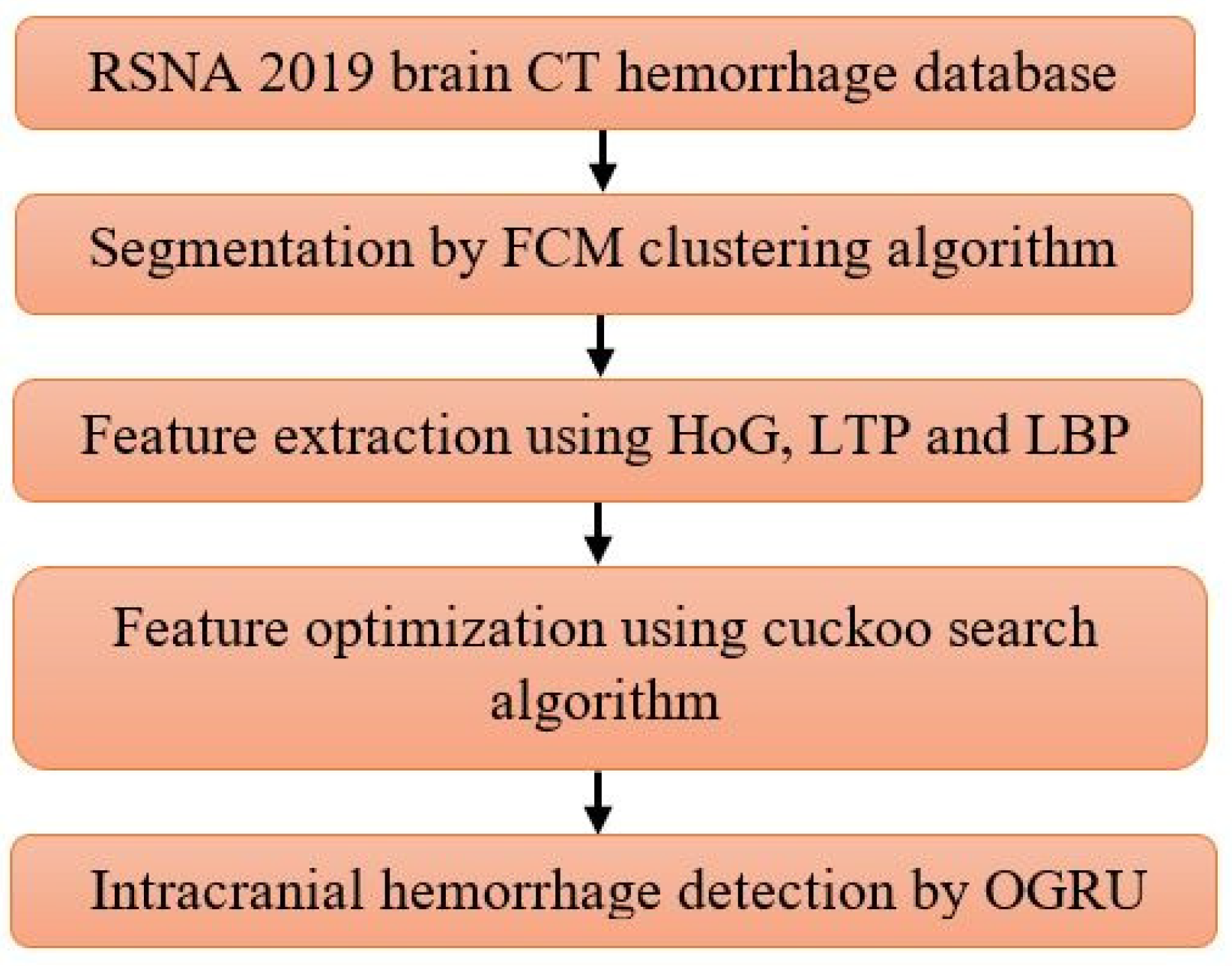
In the intracranial hemorrhage detection, the proposed system comprises five phases: Image Collection: RSNA 2019 brain CT hemorrhage database, Segmentation: FCM clustering algorithm, Feature Extraction: HoG, LTP, and LBP, Feature Optimization: Binary cuckoo search algorithm, and Classification: OGRU. The flowchart of the proposed system is illustratively specified in Figure 1.

Figure 1. Flowchart of the proposed system.

3.1. Image Collection

The proposed OGRU model’s performance is validated on a foreign database: RSNA 2019 brain CT hemorrhage database, which consists of 25,272 3D brain scans with 870,301 slices and a pixel size of $256\times 256$. In this manuscript, the proposed OGRU model is re-trained on this database, and then the results are validated with different cross-folds. In the RSNA 2019 brain CT hemorrhage database, the 3D brain scans are labeled with the annotators using 5 brain hemorrhage label types intraparenchymal, epidural, intraventricular, subarachnoid, and subdural. Furthermore, the brain scans are collected from three institutions like Stanford University, Universidade Federal de Sao Paulo Institution, and Thomas Jefferson University Hospital. In the RSNA 2019 brain CT hemorrhage database, the annotators have no information about symptoms’ acuity, medical history, patient age, and prior examination. However, it is automatically labeled as intracranial hemorrhage, while a slice comprises at least one intracranial hemorrhage type. The sample acquired 3D brain scans are depicted in Figure 2.

Figure 2. Sample acquired 3D brain scans, (a) intraparenchymal, (b) epidural, (c) intraventricular, (d) subarachnoid, and (e) subdural.

3.2. Image Segmentation

After collecting the 3D brain scans, the image segmentation is accomplished using the FCM clustering algorithm to localize the specific object in the complex templates. Hence, the FCM uses fuzzy-set theory to assign a data object to the clusters. In the FCM clustering algorithm, each object is considered a member of each cluster with a variable degree of membership. The similarity between the object is estimated by utilizing the Euclidian distance measure, which plays a crucial role to select the precise clusters. In every iteration, the objective function $j$ is reduced in the FCM clustering algorithm that is defined in Equation (1).

$$j={\displaystyle \sum }_{i=1}^N{\displaystyle \sum }_{j=1}^C{\delta }_{ij}\Vert x_{di}-c_j\Vert {}^2$$

(1)

where $C$ indicates clusters, ${\delta }_{ij}$ states degree of membership for $i^{th}$ data point $x_{di}$ in the cluster $j$, $c_j$ indicates the center vector of the cluster $j$, and $N_{x_{di}}$ denotes the number of data points.

In addition, the norm $\Vert x_{di}-c_j\Vert$ estimates the similarity of data points $x_{di}$ to the center vector of the cluster $j$. Then, ${\delta }_{ij}$ is determined for a given data point $x_{di}$ using Equation (2).

$${\delta }_{ij}=\frac{1}{{\sum }_{k=1}^C{(\frac{\Vert x_{di}-c_j\Vert }{\Vert x_{di}-c_k\Vert })}^{\frac{2}{m-1}}}$$

(2)

where $m$ states the fuzziness coefficient.

Additionally, the center vector is determined using Equation (3) [21,22].

$$c_j=\frac{{\sum }_{i=1}^N{\delta }_{ij}^m\times x_{di}}{{\sum }_{i=1}^N{\delta }_{ij}^m}$$

(3)

The fuzziness coefficient $m$ estimates the clustering tolerance by utilizing Equations (2) and (3). The limited fuzziness coefficient $m$ value has a smaller overlap between the clusters $C$. In this clustering algorithm, the accuracy $a$ is estimated by using ${\delta }_{ij}$ from the present iteration $k$ to the next iteration $k+1$, which is mathematically specified in Equation (4).

$$a={\Delta }_i^N{\Delta }_i^C\left|{\delta }_{ij}^{k+1}-{\delta }_{ij}^k\right|$$

(4)

where ${\delta }_{ij}^k$ and ${\delta }_{ij}^{k+1}$ indicates the degree of membership of the iterations $k$ and $k+1$, and $\Delta$ specifies the highest vector value. Furthermore, the hybrid feature extraction is accomplished using HoG, LBP, and LTP descriptors for extracting features from the segmented images. The sample segmented 3D brain scans are depicted in Figure 3.

Figure 3. Sample segmented 3D brain scans.

3.3. Hybrid Feature Extraction

After image segmentation, the hybrid feature extraction is accomplished by using HoG, LBP, and LTP feature descriptors, where these descriptors are selected based on the feature importance calculation. In image processing applications, the HoG descriptor is often used for extracting feature values from medical images. In the HoG feature descriptor, the magnitude, and orientation of the brain scans $I_N$ are initially computed. The vertical gradient $G_v$ and horizontal gradient $G_h$ are mathematically specified in Equation (5).

$$G_v=I_N\times {\left[-1,0,1\right]}^T, G_h=I_N\times \left[-1,0,1\right]$$

(5)

The computed vertical gradient $G_v$ and horizontal gradient $G_h$ are utilized to calculate the gradient magnitude $M\left(x,y\right)$ and angular orientation $\theta \left(x,y\right)$ that are defined in Equations (6) and (7).

$$M\left(x,y\right)=\sqrt{G_v^2\left(x,y\right)+G_h^2\left(x,y\right)}$$

(6)

$$\theta \left(x,y\right)=ta{n}^{-1}\left(\frac{G_v\left(x,y\right)}{G_{h }\left(x,y\right)}\right)$$

(7)

The gradient magnitude $M\left(x,y\right)$ and angular orientation $\theta \left(x,y\right)$ partitions the 3D brain scans into different cells. Furthermore, the orientation related to the similar cells is integrated and quantized into final histogram bins and then the respective bins are combined into the final histogram [23,24]. The total number of features $T_{hog}$ are estimated by utilizing Equation (8).

$$T_{hog}=B_{img}\times B_s\times N_b$$

(8)

where $N_b$ represents the number of bins, $B_{img}$ specifies the number of blocks per 3D brain scan, and $B_s$ denotes block size.

In addition, the LBP and LTP encode the relation between the neighborhood pixel and the referenced pixel by calculating the gray-level difference. The LBP is an effective texture feature descriptor, which transforms the 3D brain scans into labels based on luminance value. In a 3D brain scan $I$, the position of the pixel is represented as $\left(x,y\right)$, which is derived by utilizing the central pixel value $x_c$ of the threshold to signify the neighborhood pixel $n_p$. Additionally, the binary pixel value is weighted using the power of two, and further, the value is summed to generate a decimal number and it is stored in the location of $x_c$. The LBP is mathematically specified in Equations (9) and (10) [25].

$$LBP \left(x,y\right)={\displaystyle \sum }_{i=0}^{n_p-1}I{(x_i-x_c)}^{2i}, I\left(x\right)=\left\{\begin{array}{c}1, x\ge 0\\ 0, x\le 0\end{array}\right\}$$

(9)

$$U\left(LBP\left(x,y\right)\right)=\left|I\left(x_{c-1}-x_i\right)-I\left(x_0-x_i\right)\right|+{\displaystyle \sum }_{i=1}^{n_p-1}\left|I\left(x_c-x_i\right)-I\left(x_{c-1}-x_i\right)\right|$$

(10)

where $u$ denotes maximum jumping time and $x_i$ specifies the gray-level value of the center pixel $x_c$.

Similarly, the LTP is an extension of LBP that uses a thresholding constant for the pixel intensify values of three. In the LTP feature descriptor, the thresholding value is defined by using Equation (11) [26].

$$\{\begin{array}{cc}1& if n_p>x_c+T_v\\ 0& if n_p>x_c-T_v and n_p<x_c+T_v\\ -1& if n_p<x_c-T_v\end{array}$$

(11)

where $T_v$ denotes thresholding constant. By contrast, the extracted 9824 feature vectors are given as the input to the binary cuckoo search algorithm for feature optimization. The graphical representation of the feature importance calculation is shown in Figure 4.

Figure 4. Feature importance calculation.

3.4. Feature Optimization

After feature extraction, the feature optimization is accomplished using the binary cuckoo search algorithm that is stimulated using obligate parasites. In the host bird nests, the cuckoo birds lay down their eggs. The cuckoo bird mimics the external properties of the eggs from the host nests, such as color, spot, and size, and further, the cuckoo bird place the eggs in the host bird’s nests. When this approach is ineffective, the host birds identify the cuckoo eggs. Then, the host birds abandon the nest or throw away cuckoo eggs, or else the cuckoo is successful in its strategies and process for the next generation. Based on this concept, the cuckoo search algorithm is generated [27,28] and the step-by-step process of this algorithm is given below:

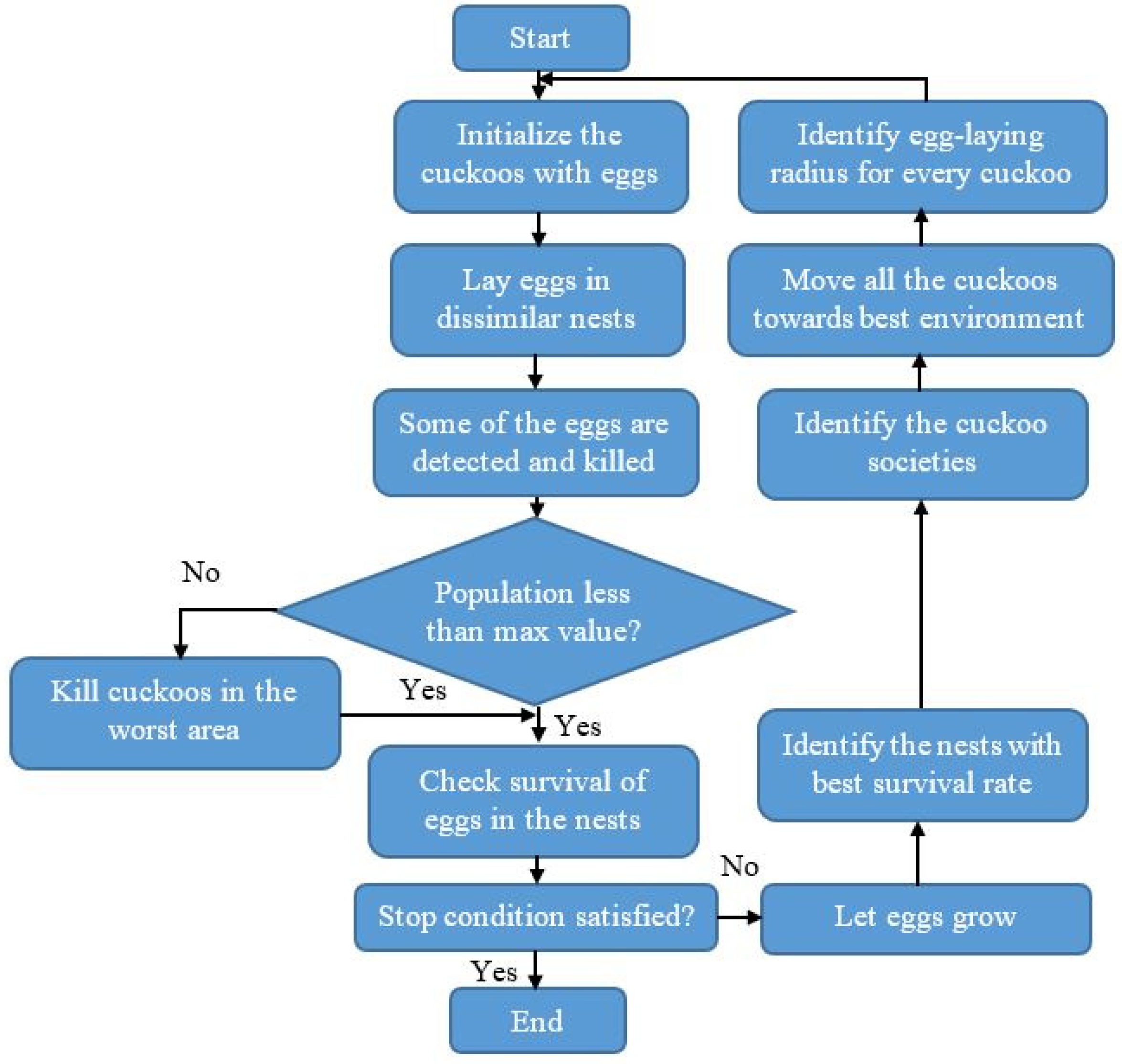
Initialization Stage: Firstly, the host nest population $P_i$ is selected randomly (where $i=1, 2\dots n$).

Generation of New Cuckoo Stage: After randomly initializing the nest population in search space, the initialized cuckoos are assessed by utilizing an objective function for identifying better solutions.

Fitness Evaluation Stage: Compute the fitness based on Equation (12) that helps to select the best one. Where,$F_L$ indicates feature length,$V$ denotes the state vector of the chaotic system and $\tilde{V}$ represents the state vector of the estimated system.

$$Fitness=\sqrt{\frac{1}{F_L}{\displaystyle \sum }_1^{F_L}{(V-\tilde{V})}^2}$$

(12)

Updating Stage: Cosine transform is employed to revise the initial solution of levy flights. A nest is chosen randomly and the excellence of the novel solution is assessed. In case, if the excellence of the new solution is superior to the old solution. The old solution is replaced with the new solution; otherwise, consider the old solution as the best solution. The levy flight used by the cuckoo search algorithm is mathematically represented in Equation (13).

$$P_i^{*}=P_i^{\left(k+1\right)}=P_i^{\left(k\right)}+\alpha \oplus Levy\left(n\right)$$

(13)

The Levy flight Equation (13) with Gaussian distribution is shown in Equations (14) and (15).

$$P_i^{*}=P_i^{\left(k+1\right)}=P_i^{\left(k\right)}+\alpha \oplus {\sigma }_s$$

(14)

$${\sigma }_s={\sigma }_{0}exp\left(-\mu \times c_g\right)$$

(15)

where ${\sigma }_0 and \mu$ indicates constant value and $c_g$ denotes the current generation.

Reject Worst Nest Stage: In this stage, the novel nests are generated randomly, and the worst nests are thrown away based on the possible values. Additionally, the best solutions are graded based on a fitness function. Finally, the best solutions are spotted and recognized as optimal solutions.

Stopping Criterion Stage: This process is replicated until the maximum iteration is accomplished.

Immigration of Cuckoos: Once the cuckoos are grown and become mature; they live in their area and society for a certain period. The best profit society value is selected after the cuckoo groups are formed in dissimilar areas. It is hard to recognize which cuckoo belongs to which group when mature cuckoos live all over the environment. To avoid this concern, cuckoo grouping is carried out using the decision tree method. Each cuckoo $\beta$ flies toward the goal habitat with a deviation of $\varnothing$ radians. These two parameters, $\beta$ and $\varnothing ,$ help cuckoos identify their positions in the environment. For each cuckoo, $\beta$ and $\varnothing$ are determined by using the Equations (16) and (17).

$$\beta \sim U\left(0,1\right)$$

(16)

$$\varnothing \sim U\left(-w,w\right)$$

(17)

where $\beta$ indicates the random number, $w$ denotes the parameter, which compels the deviation from the goal habitat.

The parameter settings of the cuckoo search algorithm are given as follows: iteration is 100, step length is 0.01, Levy flight distribution parameter is 1.5, the number of the nest is 20, the number of transition groups is 8, transition separation coefficient is 1, and transition probability coefficient is 0.1. Next, the selected 5409 feature vectors are given as the input to the OGRU model to classify six classes: Intraparenchymal, Subdural, Subarachnoid, Intraventricular, Epidural, and any other. The flowchart of the binary cuckoo search algorithm is represented in Figure 5.

Figure 5. Flowchart of the binary cuckoo search algorithm.

3.5. Classification

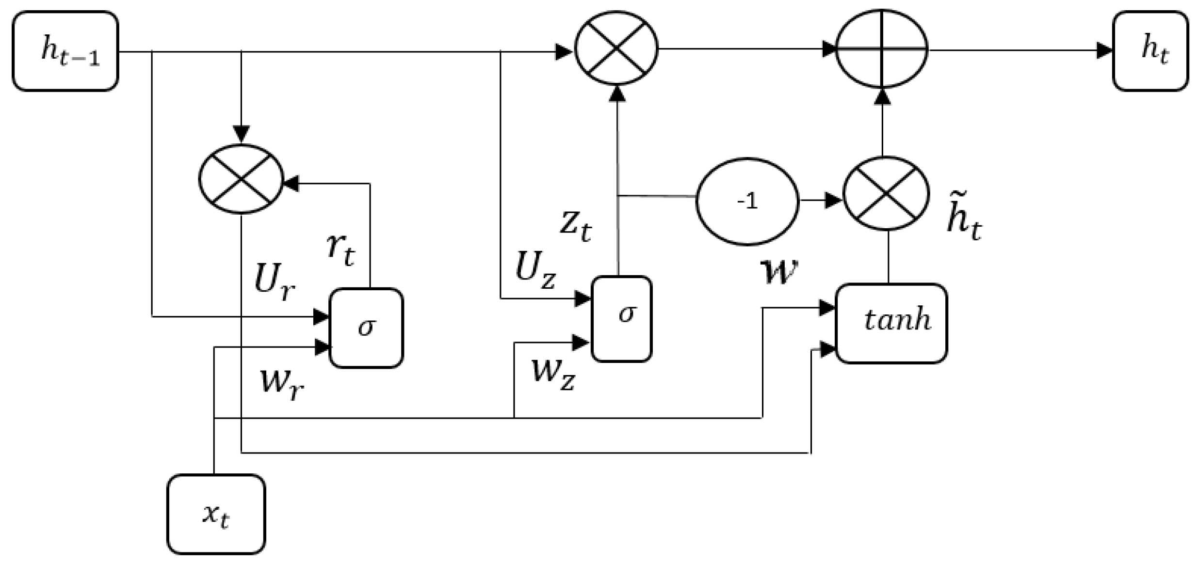
The GRU is an updated version of the Long Short Term Memory (LSTM) network that integrates forget and input gate into a single gate named the “update gate” and further, the GRU model includes an additional gate named the “reset gate”. Compared to the LSTM network, the GRU model is simple; therefore, it is becoming increasingly popular. Firstly, the GRU modulates the feature information inside the unit without using a memory cell. In the GRU model, the activation function $h_t^j$ is a linear interpolation between the previous activation $h_{t-1}^j$ and candidate activation ${\tilde{h}}_t^j$ at the time state $t$, which is mathematically specified in Equation (18) [29,30].

$$h_t^j=\left(1-z_t^j\right) h_{t-1}^j+z_t^j{\tilde{h}}_t^j$$

(18)

where $z_t^j$ represents the update gate that decides the number of units updating its activation and ${\tilde{h}}_t^j$ states candidate activation.

The mathematical expressions of the update gate and the candidate activation are defined in Equations (19) and (20).

$$z_t^j=\sigma {(w_z{A}_t+U_z{h}_{t-1})}^j$$

(19)

$${\tilde{h}}_t^j=tanh{(w{A}_t+U_r(r_t^j\times h_{t-1}))}^j$$

(20)

where $r_t^j$ states reset gates and $tanh$ states hyperbolic tangent function.

The $r_t^j$ is mathematically calculated using Equation (21).

$$r_t^j=\sigma {(w_r{A}_t+h_{t-1})}^j$$

(21)

where $w$ states parameter or weight, and $\sigma$ indicates sigmoid function.

In this scenario, the update gate $z_t^j$ controls the prior states, where the long-term dependency units are called active update gates and the short-term dependency units are called active reset gates. The Stochastic Gradient Descent (SGD) optimization algorithm is applied in the GRU model for optimizing the stochastic objective functions based on the lower-order moments. The iterative algorithm: SGD initially starts with the random point of the gradient curve, and then it slants in the slope with the help of a user-defined learning rate until the gradient curve reaches the minimum value. In this study, the SGD optimization algorithm updates the weight or parameter $w$ utilizing the gradient value $\partial L/\partial w,$ and then the corresponding gradient value is multiplied by the learning rate $\alpha$. Therefore, the updated reset gate is mathematically defined in Equation (22).

$$r_t^j=\sigma {(w_{r+1}+h_{t-1})}^j$$

(22)

where $w_{r+1}=w_r-\alpha \partial L/\partial w_r$ and the term $\partial L/\partial w_r$ states gradient loss function $L$ that reduces $w$.

If any decimal values occur, the GRU model approximately rounds off the respective decimal values into complete values. The architecture of the GRU model is specified in Figure 6.

Figure 6. Architecture of the GRU model.

The parameter settings of the GRU model are listed as follows: lambda loss amount is 0.0015, the number of hidden units are 32, the learning rate is 0.0025, and the number of iteration is 100. To resolve the un-constrained non-linear optimization issues, a BFGS algorithm is integrated with the GRU model. The BFGS algorithm uses a gradient descent function $\mu$ to further reduce the gradient value to the local minimum. The gradient descent function $\mu$ is mathematically defined in Equation (23).

$$\mu =argmin\left\{\Psi \left(\mu \right)\right\}$$

(23)

where, $\Psi \left(\mu \right)$ states non-convex function.

The point ${\mu }^{k+1}$ is computed in the next iteration $k$ using the point ${\mu }^k$, as mentioned in Equation (24).

$${\mu }^{k+1}={\mu }^k+{\vartheta }_k{d}_k$$

(24)

where $d_k$ states search direction and ${\vartheta }_k$ denotes step size, and the minimizer ${\vartheta }_k$ is mathematically defined in Equation (25).

Additionally, the search direction is specified in Equation (26).

$${\phi }_k\left(\vartheta \right)=\Psi \left({\mu }^k+\vartheta d_k\right), \vartheta >0$$

(25)

$$d_k=-S_k^{-1}{\Psi }^{\prime }\left(\mu \right)$$

(26)

where $S_k$ denotes the 2nd derivative of $\Psi$, which is called the Hessian matrix.

In this scenario, the quasi-Newton method is employed to compute $S_k$, as mentioned in Equation (27).

$$S_{k+1}{\gamma }_k={\delta }_k$$

(27)

where ${\delta }_k={\mu }^{k+1}-{\mu }^k$ and ${\gamma }_k={\Psi }^{\prime }\left({\mu }^{k+1}\right)-{\Psi }^{\prime }\left({\mu }^k\right)$.

Furthermore, the $S_k$ the approximation is computed utilizing Equation (28). The classes: Intraparenchymal, Subdural, Subarachnoid, Intraventricular, Epidural, and any other are classified based on the approximation of $S_k$. The experimental results of the OGRU-CSO model are specified in Section 4.

$$S_{k+1}=S_k-\frac{{\delta }_k{\gamma }_k^T{S}_k+S_k{\gamma }_k{\delta }_k^T}{{\gamma }_k{\delta }_k^T}+\left(1+\frac{{\gamma }_k^T{S}_k{\gamma }_k}{{\gamma }_k{\delta }_k^T}\right)\frac{{\delta }_k{\delta }_k^T}{{\delta }_k^T{\gamma }_k}$$

(28)

4. Experimental Results

In this paper, the OGRU-CSO model’s performance is simulated using MATLAB 2020a software tool on a system configuration with 16 GB random access memory, an Intel Core i9 processor, and Windows 10 operating system. The developed OGRU-CSO model’s efficiency is investigated in terms of MCC, precision, f-measure, specificity, recall, and accuracy. The mathematical formula of the undertaken performance measures is represented in Equations (29)–(34). Where, FP, FN, TP, and TN indicate false positive, false negative, true positive, and true negative:

$$Recall=\frac{TP}{TP+FN}\times 100$$

(29)

$$Precision=\frac{TP}{TP+FP}\times 100$$

(30)

$$F-measure=\frac{2TP}{FP+2TP+FN}\times 100$$

(31)

$$Accuracy=\frac{TP+TN}{TN+TP+FN+FP}\times 100$$

(32)

$$MCC=\frac{TP\times TN-FP\times FN}{\sqrt{\left(TP+FP\right)\left(TP+FN\right)\left(TN+FP\right)\left(TN+FN\right)}}\times 100$$

(33)

$$Specificity=\frac{TN}{TN+FP}\times 100$$

(34)

4.1. Quantitative Evaluation

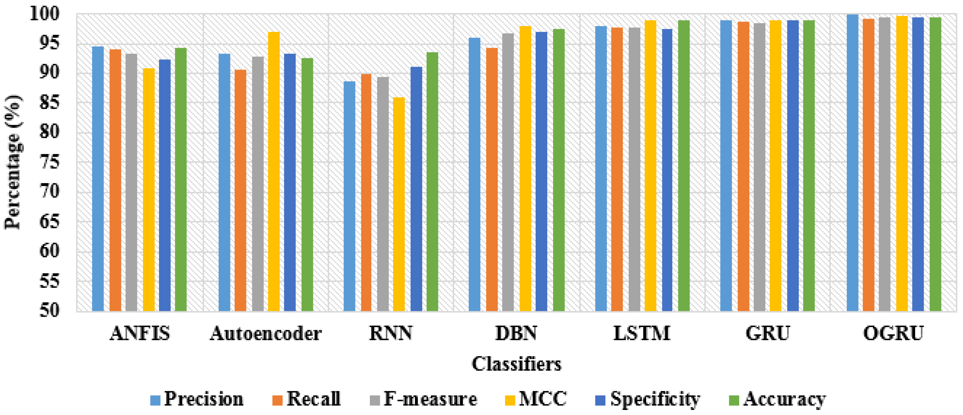
In this scenario, the efficiency of the OGRU model is validated on the RSNA 2019 brain CT hemorrhage database utilizing recall, precision, f-measure, MCC, specificity, and accuracy. By viewing Table 1 and Table 2, the performance of 7 different classifiers: LSTM, Deep Belief Network (DBN), autoencoder, Recurrent Neural Network (RNN), Adaptive Neuro-Fuzzy Inference System (ANFIS), GRU, and OGRU, are tested with the Cuckoo Search Optimization (CSO) algorithm. During the classification, similar parameters are utilized in all runs for all classifiers and a five-fold cross-validation method is applied for analyzing the performance of the OGRU model where the better use of data for training and testing decreases the computational time with limited bias and variance. The OGRU model’s performance is evaluated with two different training and testing percentages such as 50:50% and 80:20%. As stated in Table 1, the OGRU model with the CSO algorithm achieved 92.80% of precision, 90.28% of recall, 91.90% of f-measure, 92.91% of MCC, 90.88% of accuracy, and 90.48% of specificity in the intracranial hemorrhage detection with the 50% training and 50% testing of data. The obtained simulation results are better related to comparative classifiers such as LSTM, DBN, autoencoder, RNN, ANFIS, and the conventional GRU model. A graphical comparison of dissimilar classifiers with 50% training and 50% testing of data is depicted in Figure 7.

Table 1. Simulation results of the proposed model by varying the classifiers with 50:50% training and testing of data.

CSO Algorithm with 50% Training and 50% Testing of Data
Classifiers	Precision (%)	Recall (%)	F-Measure (%)	MCC (%)	Specificity (%)	Accuracy (%)
ANFIS	78.30	74.90	81.81	80.80	72.90	74.82
Autoencoder	80.88	78.50	82.88	85.55	80	82.40
RNN	82.24	80.80	86.67	86.90	82.24	84.58
DBN	86.90	84.80	86.66	87.98	86	87.77
LSTM	82.34	87.78	87.20	88.90	87.40	88.90
GRU	88.90	88.68	88.50	90.18	88.90	90.08
OGRU	92.80	90.28	91.90	92.91	90.48	90.88

Table 2. Simulation results of the proposed model by varying the classifiers with 80:20% training and testing of data.

CSO Algorithm with 80% Training and 20% Testing of Data
Classifiers	Precision (%)	Recall (%)	F-Measure (%)	MCC (%)	Specificity (%)	Accuracy (%)
ANFIS	94.50	94.09	93.40	90.83	92.30	94.32
Autoencoder	93.30	90.55	92.80	96.97	93.20	92.47
RNN	88.78	89.80	89.29	86	91.10	93.50
DBN	95.98	94.30	96.66	97.99	96.90	97.48
LSTM	97.90	97.74	97.82	98.94	97.43	98.93
GRU	98.98	98.65	98.50	99	98.98	99.04
OGRU	99.86	99.25	99.34	99.67	99.40	99.36

Figure 7. Graphical comparison of dissimilar classifiers with 50% training and 50% testing of data.

Furthermore, the RSNA 2019 brain CT hemorrhage database is categorized into train set and test set with the ratio of 80% and 20%. In the RSNA 2019 brain CT hemorrhage database, the highest performance is achieved by the OGRU model with the CSO algorithm. The developed OGRU-CSO model achieved a precision of 99.86%, recall of 99.25%, f-measure of 99.34%, MCC of 99.67%, specificity of 99.40%, and classification accuracy of 99.36%, which are superior related to other classification techniques: LSTM, DBN, autoencoder, RNN, ANFIS, and conventional GRU model. By viewing Table 2, the proposed OGRU-CSO model is highly capable of extracting and optimizing the most discriminative features, which helps in achieving better classification with limited feature vectors. A graphical comparison of dissimilar classifiers with 80% training and 20% testing of data is stated in Figure 8.

Figure 8. Graphical comparison of dissimilar classifiers with 80% training and 20% testing of data.

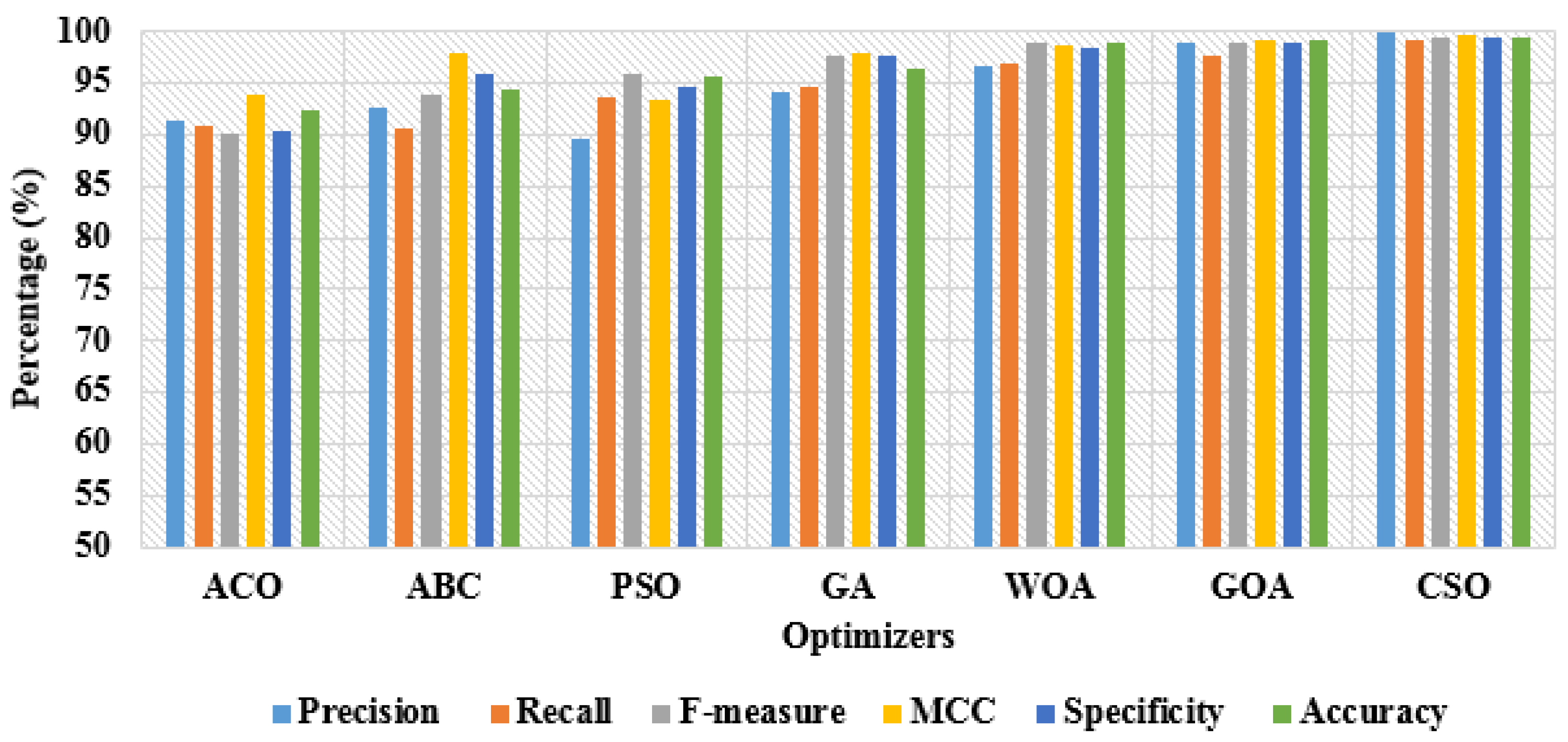
In Table 3 and Table 4, the performance investigation is conducted by using different feature optimization algorithms, such as Ant Colony Optimization (ACO), Artificial Bee Colony (ABC), Particle Swarm Optimization (PSO), Genetic Algorithm (GA), Whale Optimization Algorithm (WOA), CSO, and Grasshopper Optimization Algorithm (GOA) with OGRU model. Related to other combinations, the CSO algorithm with the OGRU attained higher results in intracranial hemorrhage detection. In this paper, the CSO algorithm significantly selects the optimum feature vectors with a better balance between exploitation and exploration. However, the comparative optimization algorithms suffer from a premature convergence rate because the optimization algorithms are stuck at the local optimal value. As seen in Table 3 and Table 4, the proposed OGRU-CSO model obtained significant performance with 80:20% training and testing of RSNA 2019 brain CT hemorrhage data compared to 50:50% training and testing of data. The graphical representation of dissimilar optimizers with 50% training and 50% testing of data is specified in Figure 9. Correspondingly, the graphical comparison of dissimilar optimizers with 80% training and 20% testing of data is denoted in Figure 10.

Table 3. Simulation results of the proposed model by varying the optimizers with 50:50% training and testing of data.

OGRU Model With 50% Training and 50% Testing of Data
Optimizers	Precision (%)	Recall (%)	F-Measure (%)	MCC (%)	Specificity (%)	Accuracy (%)
ACO	78.90	80.10	79.00	78.00	80.54	82.36
ABC	82.50	80.55	80.92	77.97	85.96	84.45
PSO	84.66	82.20	81.82	78.20	84.68	85.59
GA	88.70	84.58	84.73	79.84	87.68	86.48
WOA	88.78	86.94	85.86	80.50	88.80	88.87
GOA	88.90	87.87	88.96	82.90	89.90	89.19
CSO	92.80	90.28	91.90	92.91	90.48	90.88

Table 4. Simulation results of the proposed model by varying the optimizers with 80:20% training and testing of data.

OGRU Model with 80% Training and 20% Testing of Data
Optimizers	Precision (%)	Recall (%)	F-Measure (%)	MCC (%)	Specificity (%)	Accuracy (%)
ACO	91.40	90.90	90.00	93.80	90.40	92.30
ABC	92.50	90.50	93.90	97.90	95.90	94.40
PSO	89.70	93.50	95.85	93.29	94.67	95.55
GA	94.00	94.56	97.65	97.80	97.65	96.40
WOA	96.70	96.90	98.80	98.70	98.40	98.99
GOA	98.90	97.69	98.97	99.09	99.00	99.11
CSO	99.86	99.25	99.34	99.67	99.40	99.36

Figure 9. Graphical representation of dissimilar optimizers with 50% training and 50% testing of data.

Figure 10. Graphical comparison of dissimilar optimizers with 80% training and 20% testing of data.

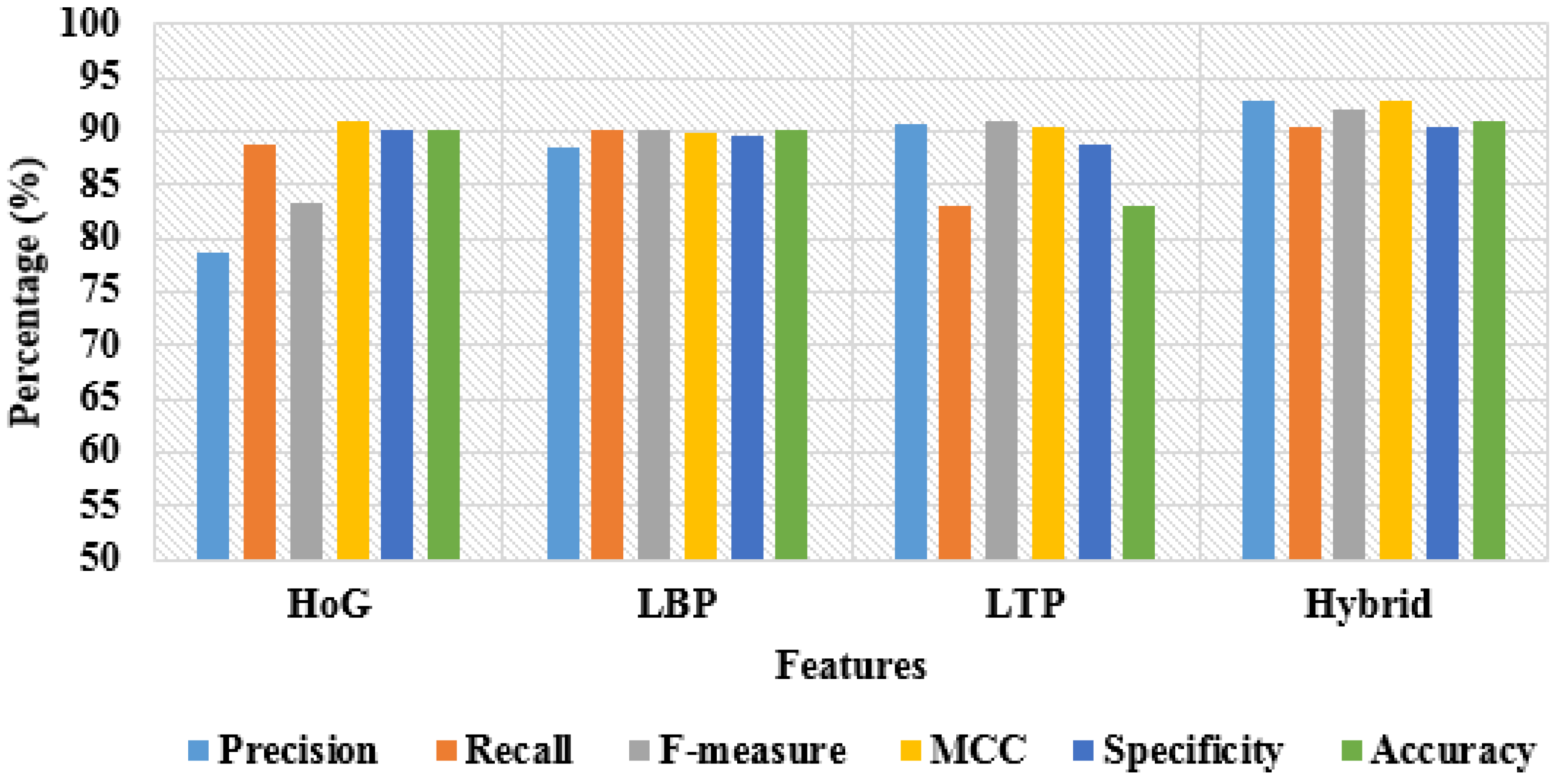
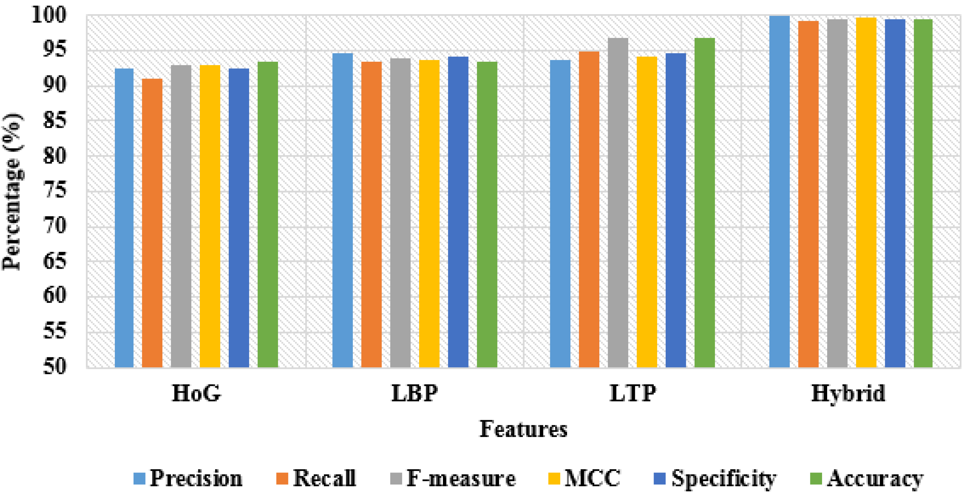
In addition, the simulation results of the proposed model by varying the features with 50:50% and 80:20% training and testing of data are depicted in Table 5 and Table 6. By inspecting the tables, the hybrid-feature extraction has achieved better classification results compared to individual feature descriptors by means of precision, recall, f-measure, MCC, specificity, and accuracy. A graphical comparison of dissimilar features with 50% training and 50% testing of data is denoted in Figure 11. In addition, the graphical comparison of dissimilar features with 80% training and 20% testing of data is represented in Figure 12.

Table 5. Simulation results of the proposed model by varying the features with 50:50% training and testing of data.

OGRU-CSO Model with 50:50% Training and Testing of Data
Features	Precision (%)	Recall (%)	F-Measure (%)	MCC (%)	Specificity (%)	Accuracy (%)
HoG	78.62	88.82	83.40	90.99	90.22	90.00
LBP	88.50	90.13	90.14	89.77	89.65	90.02
LTP	90.70	82.89	90.78	90.24	88.66	82.93
Hybrid	92.80	90.28	91.90	92.91	90.48	90.88

Table 6. Simulation results of the proposed model by varying the features with 80:20% training and testing of data.

OGRU-CSO Model with 80:20% Training and Testing of Data
Features	Precision (%)	Recall (%)	F-Measure (%)	MCC (%)	Specificity (%)	Accuracy (%)
HoG	92.52	91.09	93.02	92.87	92.43	93.36
LBP	94.55	93.43	93.94	93.55	94.08	93.42
LTP	93.72	94.88	96.77	94.20	94.60	96.90
Hybrid	99.86	99.25	99.34	99.67	99.40	99.36

Figure 11. Graphical comparison of dissimilar features with 50% training and 50% testing of data.

Figure 12. Graphical comparison of dissimilar features with 80% training and 20% testing of data.

4.2. Comparative Evaluation

Additionally, the comparative investigation between the proposed and the existing models are indicated in Table 7. Anupama et al. [10] created a novel intracranial hemorrhage detection system based on a synergic deep learning model and a Grab cut-based segmentation algorithm. Hence, the developed model has achieved 95.73% of classification accuracy, 97.78% of specificity, and 94.01% of recall on the benchmark intracranial hemorrhages detection database.

Table 7. Comparative investigation between the proposed and the existing models.

Models	Database	Accuracy (%)	Recall (%)	Specificity (%)
Synergic deep learning model [10]		95.73	94.01	97.78
ResNeXt-101 [15]		97.54	60.79	99.32
ResNeXt-101 with bidirectional LSTM [15]	RSNA 2019 brain CT hemorrhage	97.83	72.86	99
2D CNN [16]		95	95.84	94.85
OGRU-CSO		99.36	99.25	99.40

Burduja et al. [15] have combined a pre-trained CNN model named ResNeXt-101 with a bidirectional long short-term memory network for recognizing intracranial hemorrhages in 3D CT scans. The experimental results showed that the individual ResNeXt-101 model achieved 97.54% of classification accuracy, 60.79% of recall, and 99.32% of specificity. However, the ResNeXt-101 with bidirectional long short-term memory network has achieved better specificity of 99%, recall of 72.86%, and classification accuracy of 97.83% on the RSNA 2019 brain CT hemorrhage database. Wang et al. [16] developed a novel deep learning model, which integrates two sequence models and 2D CNN to achieve precise acute intracranial hemorrhage detection. However, the presented model attained specificity of 94.85%, recall of 95.84%, and classification accuracy of 95% on the benchmark intracranial hemorrhages detection database. Related to these comparative models, the developed OGRU-CSO model achieved superior results in intracranial hemorrhage detection by utilizing specificity, recall, and accuracy on the RSNA 2019 brain CT hemorrhage database. In addition to this, the selection of the optimal features by the CSO algorithm reduces the model complexity to linear. The computational time of the proposed model is 33.28 s, which is superior to other optimizers and classifiers.

5. Conclusions

In this paper, the OGRU-CSO model is developed for intracranial hemorrhage detection or segmentation in the 3D CT scans. The proposed OGRU-CSO model consists of two important phases: feature selection or optimization and classification. After segmenting the diseased portions from the collected 3D CT scans, the feature vectors are extracted using three feature descriptors such as HoG, LBP, and LTP. The extracted features are multi-dimensional, so the CSO optimization algorithm is employed for optimizing the dimension of the extracted feature vectors to improve the computation time and the system complexity. Finally, the optimized discriminative feature vectors are given as the input to the OGRU for the sub-type classification of intracranial hemorrhages. In the experimental section, the proposed OGRU-CSO model achieved 99.36% of classification accuracy on the RSNA 2019 brain CT hemorrhage database, which is effectively related to other classifiers and optimizers. Furthermore, the computational complexity of the proposed OGRU-CSO model is linear by optimizing the feature vectors. As a future extension, a novel hyper-parameter optimization algorithm can be included in the OGRU model to further enhance intracranial hemorrhage lesions detection.

References

1. Li, L.; Wei, M.; Liu, B.; Atchaneeyasakul, K.; Zhou, F.; Pan, Z.; Kumar, S.A.; Zhang, J.Y.; Pu, Y.; Liebeskind, D.S.; et al. Deep learning for hemorrhagic lesion detection and segmentation on brain CT images. IEEE J. Biomed. Health Inform. 2020, 25, 1646–1659. [Google Scholar] [CrossRef] [PubMed]
2. Remedios, S.W.; Roy, S.; Bermudez, C.; Patel, M.B.; Butman, J.A.; Landman, B.A.; Pham, D.L. Distributed deep learning across multisite datasets for generalized CT hemorrhage segmentation. Med. Phys. 2020, 47, 89–98. [Google Scholar] [CrossRef]
3. Karki, M.; Cho, J.; Lee, E.; Hahm, M.H.; Yoon, S.Y.; Kim, M.; Ahn, J.Y.; Son, J.; Park, S.H.; Kim, K.H.; et al. CT window trainable neural network for improving intracranial hemorrhage detection by combining multiple settings. Artif. Intell. Med. 2020, 106, 101850. [Google Scholar] [CrossRef] [PubMed]
4. Kuo, W.; Häne, C.; Mukherjee, P.; Malik, J.; Yuh, E.L. Expert-level detection of acute intracranial hemorrhage on head computed tomography using deep learning. Proc. Natl. Acad. Sci. USA 2019, 116, 22737–22745. [Google Scholar] [CrossRef] [PubMed]
5. Duperron, M.G.; Tzourio, C.; Schilling, S.; Zhu, Y.C.; Soumare, A.; Mazoyer, B.; Debette, S. High dilated perivascular space burden: A new MRI marker for risk of intracerebral hemorrhage. Neurobiol. Aging 2019, 84, 158–165. [Google Scholar] [CrossRef] [PubMed]
6. Imran, R.; Hassan, N.; Tariq, R.; Amjad, L.; Wali, A. Intracranial Brain Haemorrhage Segmentation and Classification. Iksp J. Comput. Sci. Eng. 2021, 1, 52–56. [Google Scholar]
7. Lee, J.Y.; Kim, J.S.; Kim, T.Y.; Kim, Y.S. Detection and classification of intracranial haemorrhage on CT images using a novel deep-learning algorithm. Sci. Rep. 2020, 10, 20546. [Google Scholar] [CrossRef]
8. Lee, H.; Yune, S.; Mansouri, M.; Kim, M.; Tajmir, S.H.; Guerrier, C.E.; Ebert, S.A.; Pomerantz, S.R.; Romero, J.M.; Kamalian, S.; et al. An explainable deep-learning algorithm for the detection of acute intracranial haemorrhage from small datasets. Nat. Biomed. Eng. 2019, 3, 173–182. [Google Scholar] [CrossRef]
9. Huang, J.L.; Woehrle, T.A.; Conway, P.; McCarty, C.A.; Eyer, M.M.; Eyer, S.D. Evaluation of a protocol for early detection of delayed brain hemorrhage in head injured patients on warfarin. Eur. J. Trauma Emerg. Surg. 2019, 45, 481–487. [Google Scholar] [CrossRef]
10. Anupama, C.S.S.; Sivaram, M.; Lydia, E.L.; Gupta, D.; Shankar, K. Synergic deep learning model-based automated detection and classification of brain intracranial hemorrhage images in wearable networks. Pers. Ubiquitous Comput. 2022, 26, 1–10. [Google Scholar] [CrossRef]
11. Raghavendra, U.; Pham, T.; Gudigar, A.; Vidhya, V.; Rao, B.N.; Sabut, S.; Wei, J.K.E.; Ciaccio, E.J.; Acharya, U.R. Novel and accurate non-linear index for the automated detection of haemorrhagic brain stroke using CT images. Complex. Intell. Syst. 2021, 7, 929–940. [Google Scholar] [CrossRef]
12. Hssayeni, M.D.; Croock, M.S.; Salman, A.D.; Al-khafaji, H.F.; Yahya, Z.A.; Ghoraani, B. Intracranial hemorrhage segmentation using a deep convolutional model. Data 2020, 5, 14. [Google Scholar] [CrossRef]
13. Ye, H.; Gao, F.; Yin, Y.; Guo, D.; Zhao, P.; Lu, Y.; Wang, X.; Bai, J.; Cao, K.; Song, Q.; et al. Precise diagnosis of intracranial hemorrhage and subtypes using a three-dimensional joint convolutional and recurrent neural network. Eur. Radiol. 2019, 29, 6191–6201. [Google Scholar] [CrossRef] [PubMed]
14. Sage, A.; Badura, P. Intracranial hemorrhage detection in head CT using double-branch convolutional neural network, support vector machine, and random forest. Appl. Sci. 2020, 10, 7577. [Google Scholar] [CrossRef]
15. Burduja, M.; Ionescu, R.T.; Verga, N. Accurate and efficient intracranial hemorrhage detection and subtype classification in 3D CT scans with convolutional and long short-term memory neural networks. Sensors 2020, 20, 5611. [Google Scholar] [CrossRef]
16. Wang, X.; Shen, T.; Yang, S.; Lan, J.; Xu, Y.; Wang, M.; Zhang, J.; Han, X. A deep learning algorithm for automatic detection and classification of acute intracranial hemorrhages in head CT scans. NeuroImage Clin. 2021, 32, 102785. [Google Scholar] [CrossRef]
17. Gautam, A.; Raman, B. Towards effective classification of brain hemorrhagic and ischemic stroke using CNN. Biomed. Signal. Processing Control 2021, 63, 102178. [Google Scholar] [CrossRef]
18. Mansour, R.F.; Aljehane, N.O. An optimal segmentation with deep learning based inception network model for intracranial hemorrhage diagnosis. Neural Comput. Appl. 2021, 33, 13831–13843. [Google Scholar] [CrossRef]
19. Kumar, I.; Bhatt, C.; Singh, K.U. Entropy based automatic unsupervised brain intracranial hemorrhage segmentation using CT images. J. King Saud Univ. Comput. Inf. Sci. 2020, 34, 2589–2600. [Google Scholar] [CrossRef]
20. Patel, A.; Leemput, S.C.V.D.; Prokop, M.; Ginneken, B.V.; Manniesing, R. Image level training and prediction: Intracranial hemorrhage identification in 3D non-contrast CT. IEEE Access 2019, 7, 92355–92364. [Google Scholar] [CrossRef]
21. Huang, H.; Meng, F.; Zhou, S.; Jiang, F.; Manogaran, G. Brain image segmentation based on FCM clustering algorithm and rough set. IEEE Access 2019, 7, 12386–12396. [Google Scholar] [CrossRef]
22. Dubey, Y.K.; Mushrif, M.M. FCM clustering algorithms for segmentation of brain MR images. Adv. Fuzzy Syst. 2016, 2016, 3406406. [Google Scholar] [CrossRef]
23. Kapoor, R.; Gupta, R.; Son, L.H.; Jha, S.; Kumar, R. Detection of power quality event using histogram of oriented gradients and support vector machine. Measurement 2018, 120, 52–75. [Google Scholar] [CrossRef]
24. Nigam, S.; Singh, R.; Misra, A.K. Efficient facial expression recognition using histogram of oriented gradients in wavelet domain. Multimed. Tools Appl. 2018, 77, 28725–28747. [Google Scholar] [CrossRef]
25. Turkoglu, M.; Hanbay, D. Leaf-based plant species recognition based on improved local binary pattern and extreme learning machine. Phys. A: Stat. Mech. Its Appl. 2019, 527, 121297. [Google Scholar] [CrossRef]
26. Kanwal, N.; Girdhar, A.; Kaur, L.; Bhullar, J.S. Digital image splicing detection technique using optimal threshold based local ternary pattern. Multimed. Tools Appl. 2020, 79, 12829–12846. [Google Scholar] [CrossRef]
27. Mareli, M.; Twala, B. An adaptive Cuckoo search algorithm for optimisation. Appl. Comput. Inform. 2018, 14, 107–115. [Google Scholar] [CrossRef]
28. Cuong-Le, T.; Minh, H.L.; Khatir, S.; Wahab, M.A.; Tran, M.T.; Mirjalili, S. A novel version of Cuckoo search algorithm for solving optimization problems. Expert Syst. Appl. 2021, 186, 115669. [Google Scholar] [CrossRef]
29. Chen, J.; Jing, H.; Chang, Y.; Liu, Q. Gated recurrent unit based recurrent neural network for remaining useful life prediction of nonlinear deterioration process. Reliab. Eng. Syst. Saf. 2019, 185, 372–382. [Google Scholar] [CrossRef]
30. Xu, C.; Shen, J.; Du, X.; Zhang, F. An intrusion detection system using a deep neural network with gated recurrent units. IEEE Access 2018, 6, 48697–48707. [Google Scholar] [CrossRef]
Publisher’s Note: MDPI stays neutral with regard to jurisdictional claims in published maps and institutional affiliations.
Article Metrics
Citations
Article Access Statistics
Multiple requests from the same IP address are counted as one view.