Real-Time Prediction Model of Carbon Content in RH Process

Abstract

In the Ruhrstahl–Heraeus (RH) vacuum degassing process, we propose a real-time prediction model for the carbon content in molten steel, and show that the decarburization endpoint can be accurately determined using this model. Firstly, we applied a novel off-gas analyzer that can measure the carbon oxide concentration produced in the decarburization reaction faster and more accurately. Next, we generate decarburization curves using the off-gas components measured by the new analyzer. The decarburization curve describes the carbon content profile well during operation, and shows good agreement with the actual carbon content. In order to predict the carbon content during operation in real time, we create an artificial neural network (ANN) using the decarburization curves and operation data. By comparing the endpoint carbon content measured at the end of the operation with the predicted values, we confirmed the excellent predictive performance of the ANN model. Finally, we show that it is possible to accurately determine the decarburization endpoint using the prediction model. We expect that the proposed real-time prediction model can increase the productivity of the RH process.

1. Introduction

The Ruhrstahl–Heraeus (RH) vacuum degassing process is a kind of secondary steelmaking process between the Basic Oxygen Furnace (BOF) and the Continuous Casting (CC) process [1,2,3,4]. It aims to improve the cleanliness of steel by reducing impurities such as hydrogen, nitrogen and oxygen. It also controls the temperature of the molten steel to achieve the requirement of the CC process. In particular, due to the excellent decarburization capability of the RH process, it is the most popular vacuum steel refining unit for the production of Ultra-Low Carbon (ULC) steel and Interstitial Free (IF) steel for automobiles [5,6,7,8].

In order to produce high-quality ULC steel, it is important to estimate the decarburization rate of the molten steel during the operation and to determine the decarburization end time exactly. If the operation is terminated too early due to the incorrect prediction of the decarburization rate, the mechanical and chemical properties of steel products may deteriorate due to the high carbon content and additional work may be required to remove the residual carbon in the melt. In contrast, if the operation time is delayed longer than necessary, the consumption of utilities such as circulation gas, ejection steam and electricity increases and the erosion of refractory materials in the vacuum chamber and submerged snorkels accelerates. Since the temperature of the molten steel may become too low due to the excessively long operating time, it may take additional energy and time to reheat the molten steel. In addition, some ULC steels, such as Bake Hardened (BH) steel [9], have very narrow upper and lower limits of target carbon content, so it is necessary to determine the decarburization end time through more accurate estimation of the decarburization rate.

Because it is difficult to measure the dissolved carbon content of the molten steel in real time, process operators typically rely on intermittent sampling measurements or their long experience to estimate the dissolved carbon content during the RH process. So there have been various studies to predict the decarburization rate accurately and to understand the degassing reaction in the RH process.

Based on mass and thermal balance, the decarburization reaction can be expressed as a first-order equation with the apparent rate constant of decarburization [10,11,12,13]. Many studies have attempted to determine the influence of various factors affecting the apparent rate constant of decarburization, such as circulation flow rate, initial carbon and oxygen concentration, internal pressure of vacuum chamber and flow rate of Top Oxygen Blowing (TOB) [11,14,15,16,17,18]. In addition, they have tried to obtain sophisticated prediction models by identifying decarburization mechanisms according to the reaction zone where the decarburization reactions take place and by analyzing changes in decarburization rates over operating time [5,14,17,19,20,21]. However, the RH process involves multidimensional physicochemical phase changes at high temperature and the model parameters may change depending on the capacity and conditions of the equipment. Therefore, it is difficult to obtain a generalized model through experiments, especially in large-scale commercial facilities where experiments are time-consuming and expensive.

Some researchers have used Computational Fluid Dynamics (CFD) to calculate nonlinear reactions in the RH processes, taking into account various operating conditions that are difficult to test directly. CFD is particularly effective in identifying decarburization rates according to reaction area or operating time and in finding optimal process conditions such as circulation flow rate, oxygen blowing and snorkel dimensions [22,23,24]. However, the CFD models have limitations to account for all important responses due to computational power, lack of prior knowledge of the system, or modeling complexity. In addition, they are often not suitable for real-time prediction due to inaccurate or excessive assumptions used in the model [15,25].

Other researchers have studied data-driven modeling that combines real-time data collected from various sensors and machine learning algorithms. Kim et al. [26,27] use Fuzzy logic to predict the end point of decarburization in the middle of the RH operation. They have selected the main factors affecting the operating time through correlation analysis and multiple regression analysis and have constructed separate Fuzzy models according to the steel type. The prediction model learns the actual decarburization endpoint by the operator and does not account for changes in dissolved carbon content during operation. Kleimt et al. [28,29] propose a dynamic model of the RH process for online observation and model-based control. They calculate thermodynamic equilibrium and reaction kinetics by considering the cyclic process data and acyclic event data. The model shows excellent performance in predicting the decarburization rate as well as impurities and temperature changes of molten steel. However, there is a limit to obtaining a generalized model because the parameter identification of the physical model must be preceded. Zhang et al. [30] attempt to calculate the dissolved carbon content in real time during RH operations using the operator’s experience, metallurgical knowledge and operational data. Jianwen et al. [31] tried to predict the endpoint carbon content using the Radial Basis Function (RBF) neural network in a Vacuum Oxygen Decarburization (VOD) vacuum steel refining process. However, these studies show relatively large prediction errors due to the lack of consideration for the actual change in dissolved carbon content during operation. In addition to the RH process, the data-driven models are actively used in various fields of the steelmaking process and studies have been reported to predict the change of impurities [32,33,34] and temperature [35] of the molten steel. However, the difficulty of collecting dissolved carbon content data poses an obstacle to developing real-time prediction models in the RH process. In other words, it is not only difficult to measure the continuous change in the dissolved carbon during operation, but it is also time-consuming and expensive to obtain the actual carbon content under various operating conditions.

In this work, we proposed a real-time prediction model for carbon content in molten steel using real-time operation data and the carbon oxide content in off-gas and showed that the decarburization end time could be accurately determined using the model. The main idea of this study is that carbon oxides emitted through the off-gas in the RH process come only from molten steel. If we know exactly the amount of carbon oxides in the off-gas at any given time, we can accurately infer the decarburization reaction rate at that time. However, the off-gas analyzer used in the general RH process is installed far from the vacuum chamber where the decarburization reaction takes place, so it is difficult to capture the decarburization reaction in the molten steel in time. So we firstly introduced a new type of gas analyzer, Tunable Diode Laser Absorption Spectroscopy (TDLAS), to the RH process and showed that the off-gas components emitted from the vacuum chamber could be measured faster and more accurately by using it. Next, we introduced a decarburization curve to estimate the carbon concentration in the molten steel using carbon monoxide and carbon dioxide concentrations in the off-gas measured by the TDLAS analyzer and confirmed the similarity between the results of the decarburization curve and the actual sampling data. Since the decarburization curve can be obtained after an operation is over, it cannot be used for online prediction. Instead, we used Artificial Neural Networks (ANNs) as an online prediction model for carbon content in the molten steel. We had trained the ANN model by using the process data obtained during operations and the decarburization curves as input and output values, respectively. Finally, we compared the actual carbon concentrations at the end of decarburization with the predicted values of the ANN model to confirm the validity of the prediction model.

This paper is organized as follows. Section 2 describes the use of the TDLAS analyzer in the RH process and the method of developing a real-time prediction model for dissolved carbon content using off-gas measurement. Section 3 evaluates the measurement performance of the TDLAS analyzer and validates the accuracy of the carbon concentrations in molten steel using the proposed prediction model. Section 4 provides conclusions and future scope.

2. Materials and Methods

2.1. Method Overview

The procedure performed in this paper to develop a real-time decarburization model can be summarized as follows:

• A new method to measure CO and CO₂ concentrations in the off-gas

  (a)

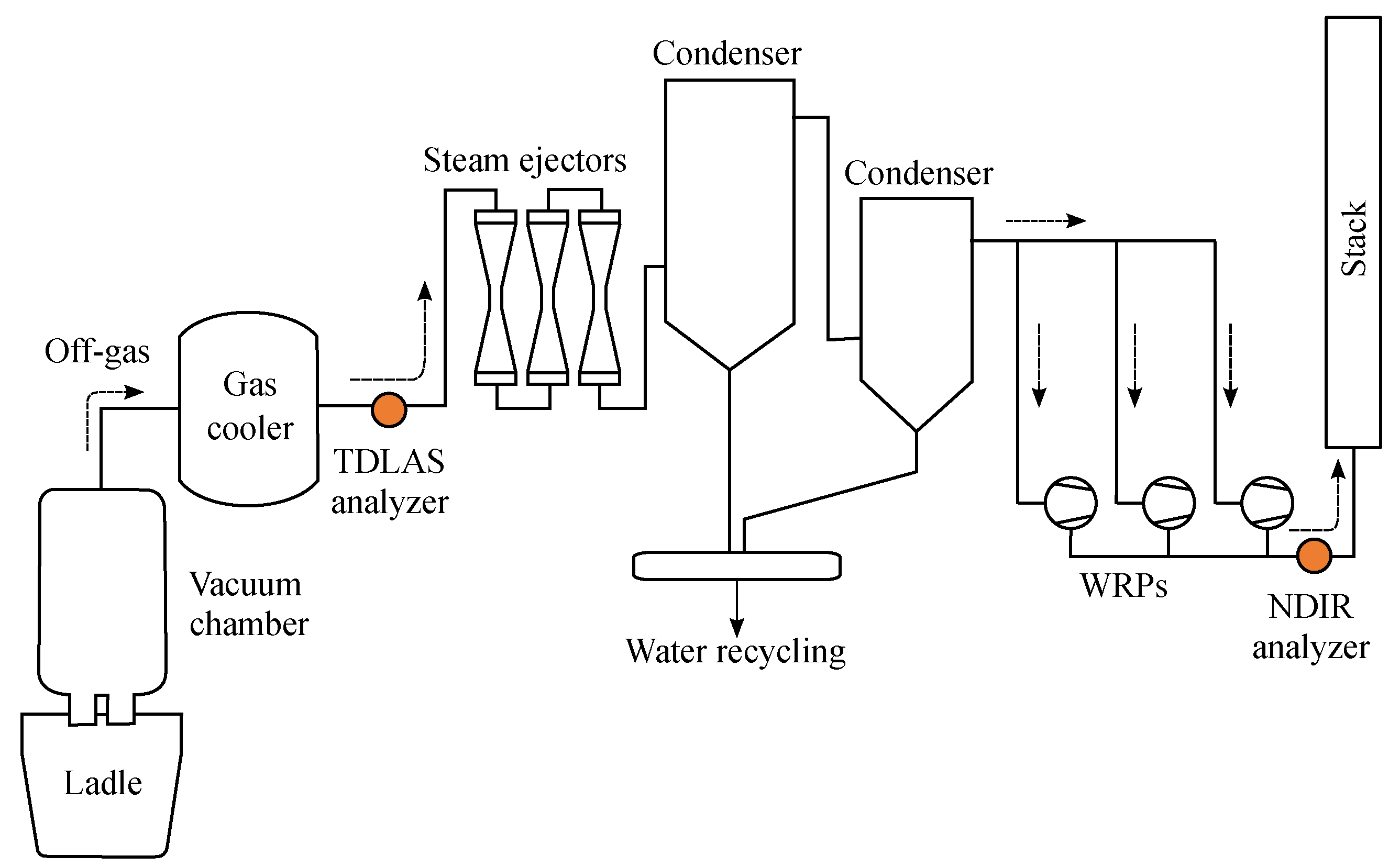
  Application of a new off-gas analyzer close to the vacuum chamber

  (b)

  Comparison and verification of measurement results

• Offline decarburization model

  (a)

  Construction and verification of decarburization curves of molten steel

• Online prediction model

  (a)

  Training the ANN model using the decarburization curve as the target value

  (b)

  Verification using endpoint carbon contents

• Determination of the decarburization endpoint using online predictive model

2.2. RH Vacuum Degassing Process

The RH vacuum degasser consists of a vacuum chamber with two snorkels at the bottom, vacuum facilities consisting of Water Ring Pumps (WRPs) and steam ejectors and alloy hoppers for injecting alloy ores (Figure 1). Once the ladle containing the molten steel is located under the vacuum chamber, the chamber descends to submerge the snorkels into the melt. The circulation gas (typically argon) is introduced into one of the two snorkels through gas lines installed in a circumferential direction of the snorkels and at the same time, the pressure inside the vacuum chamber is finally lowered to 1 kPa or less by using vacuum facilities. Due to the buoyancy of the circulation gas and the low pressure inside the vacuum chamber, the molten steel in the ladle rises to the vacuum chamber through the snorkels into which the circulation gas is injected.

In the vacuum chamber, impurities such as nitrogen, hydrogen and carbon present in the molten steel are removed in a gaseous state due to the difference of gas partial pressure between the atmosphere and the melt. The molten steel inside the vacuum chamber is returned to the ladle through the opposite snorkel and this circulation process is repeated until the impurities in the molten steel are lowered to the desired level. The carbon component combines with oxygen present in the molten steel and is emitted in the form of carbon monoxide (CO) or carbon dioxide (CO₂). In some cases, the TOB installed on the top or side of the vacuum chamber can accelerate the decarburization reaction by supplying additional oxygen to the surface of the molten steel at high speed [15,36].

The main decarburization reactions are as follows:

$$\begin{array}{cc}\hfill \left[\mathrm{C}\right]+\frac{1}{2}\left\{{\mathrm{O}}_2\right\}& ⟶\left\{\mathrm{CO}\right\}\hfill \\ \hfill \left[\mathrm{C}\right]+\left[\mathrm{O}\right]& ⟶\left\{\mathrm{CO}\right\}\hfill \\ \hfill \left\{\mathrm{CO}\right\}+\frac{1}{2}\left\{{\mathrm{O}}_2\right\}& ⟶\left\{{\mathrm{CO}}_2\right\}\hfill \end{array}$$

(1)

where the brackets and braces represent the dissolved and gaseous states of their corresponding components, respectively. In actual operations, operators use the CO and CO₂ concentrations contained in the off-gas as an auxiliary means to predict the decarburization rate in the molten steel.

2.3. Measurement of the Carbon Oxide Concentration

As shown in Figure 1, we measured CO and CO₂ concentrations in the off-gases using two types of gas analyzers: Non-Dispersive Infra-Red (NDIR) and TDLAS. Both are IAS (Infrared Absorption Spectrograph), meaning they use the property that different gas species absorb different wavelengths of light. The concentration of a specific gas is measured by detecting the intensity of the light emitted by the analyzer being absorbed or transmitted by the gas component. Analyzers using IAS are classified according to the type of light source and signal processing method.

The NDIR spectrograph [37,38,39] is the most commonly used analyzer for measuring the concentration of gas components in the RH process. It consists of an infrared source, a sample cell containing the gas of interest, a reference cell containing an inert gas and a detector. The light emitted from the broadband light source is split into two branches and passes through the sample cell and the reference cell, respectively. We can calculate the concentration of the gas of interest using the difference in intensity between the two beams passing through the two cells. Even though this method is an easy and inexpensive method widely used for off-gas measurement in steelmaking processes, it is sensitive to disturbances such as dust, humidity, temperature changes and pressure changes and has limitations in harsh environments and in situ measurement. Therefore, the NDIR analyzers are typically installed at the end of the exhaust line of the RH process to minimize disturbances, which causes a time delay in detecting changes in the off-gas composition occurring in the vacuum chamber.

The TDLAS analyzer has been expanding its applications in various industries such as petrochemicals, power plants and steelmaking processes due to its excellent wavelength selectivity and strong resistance to disturbances [40,41,42,43,44,45,46,47,48,49,50,51,52]. It emits a monochromatic laser beam of a specific wavelength absorbed by the sample gas from the diode laser (transmitter) and measures the intensity of light passing through the sample using a detector (receiver). By measuring the absorption spectrum while varying the wavelength of the laser, it is possible to reduce the influence of background noise and disturbance and improve measurement accuracy. In addition, the TDLAS analyzer measures the gas concentration within a volume determined by the laser beam width and Optical Path Length (OPL), which reduces the measurement error due to the uneven gas mixtures, resulting in more reliable gas composition. These features allow direct measurement of the off-gas concentrations inside the exhaust line in situ, even in harsh environments.

In this work, we used two TDLAS analyzers to measure both CO and CO₂ concentrations and installed them in a cross duct configuration to measure the gas concentration in the center of the exhaust duct. We installed the TDLAS analyzers on the rear of the gas cooler close to the vacuum chamber; there it was less affected by dust and also used the existing NDIR analyzers installed near the stack at the end of the exhaust line.

2.4. Estimation of the Carbon Content in the Molten Steel

The RH process requires high airtightness between the vacuum chamber and the exhaust line to obtain a high vacuum. Therefore, the amount of air flowing in or out of the process is very small and we assume that CO and CO₂ observed in the exhaust line only occur inside the molten steel. That is, if we know the total amount of carbon oxides emitted from the molten steel, it is possible to estimate the total amount of decarburization of the molten steel. Using the real-time carbon oxide concentration during the RH operation, we calculated the carbon concentration of the molten steel over time as follows:

$$\begin{array}{cc}\hfill {\left[\mathrm{C}\right]}_t& ={\left[\mathrm{C}\right]}_{t-1}-({\left\{\mathrm{CO}\right\}}_t+{\left\{{\mathrm{CO}}_2\right\}}_t)\times \alpha \hfill \end{array}$$

(2)

$$\begin{array}{cc}\hfill \alpha & =\frac{{\left[\mathrm{C}\right]}_{t_0}-{\left[\mathrm{C}\right]}_{t_f}}{{\sum }_{t=t_0}^{t_f}({\left\{\mathrm{CO}\right\}}_t+{\left\{{\mathrm{CO}}_2\right\}}_t)}\hfill \end{array}$$

(3)

where [C]${}_t$ is the dissolved carbon concentration (ppm) in the molten steel at time t, {CO}${}_t$ and {CO₂}${}_t$ are the concentrations (%) of the carbon oxides in the off-gas measured at time t and $t_0$ and $t_f$ are the start and end time of the decarburization process, respectively. Moreover, $\alpha$ is a conversion factor that converts the measured CO and CO₂ concentrations in the off-gas to the amount of decarburization in the molten steel.

We can obtain decarburization curves over time from the initial and final carbon concentrations in the molten steel and the real-time measurement of CO and CO₂ concentrations. In order to confirm the consistency of the decarburization curves obtained using Equation (2), we selected 12 decarburization operations and sampled the molten steel at intervals of 1–2 min during the decarburization operations to measure the actual amount of dissolved carbon.

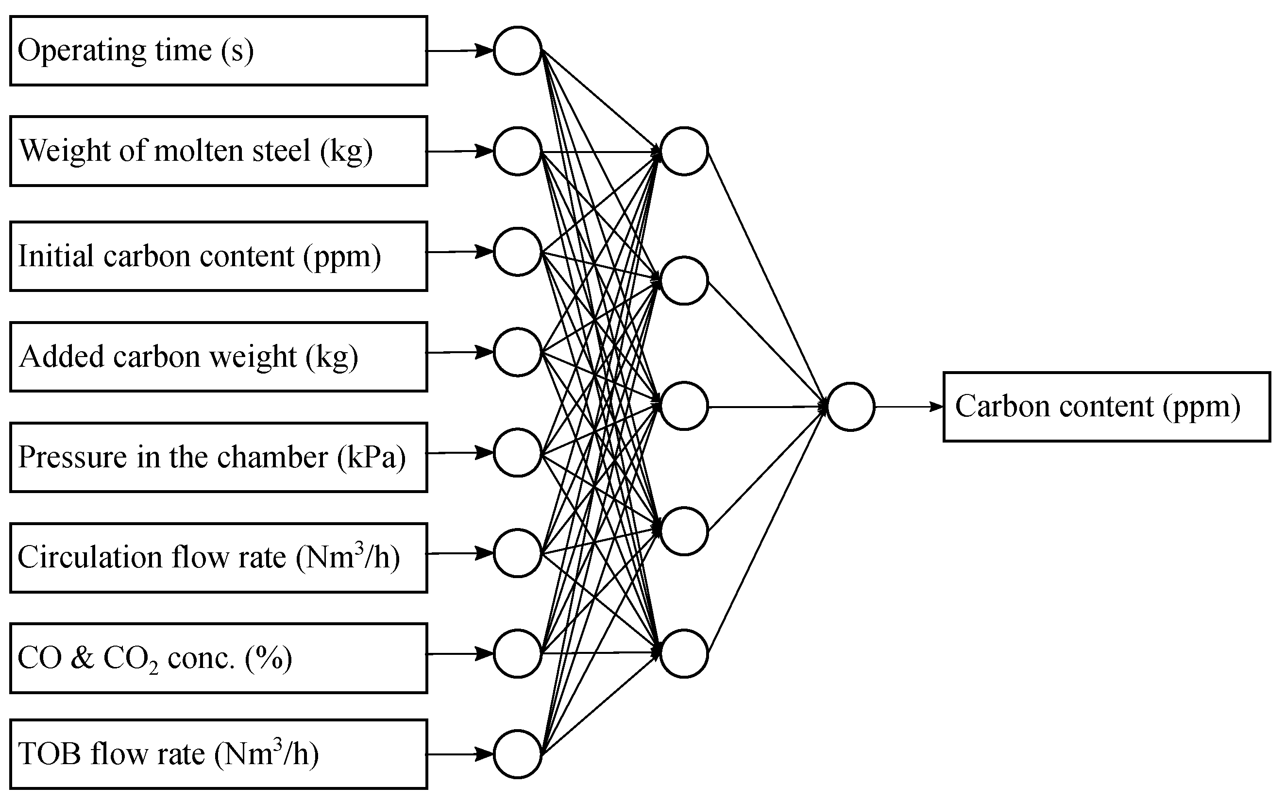
2.5. Artificial Neural Network Model

To calculate the decarburization curves using Equation (2), it is necessary to know the final carbon concentration in the molten steel and the total amount of carbon oxides emitted during the entire operating period. Therefore, we cannot directly use Equation (2) to predict the real-time decarburization rate during operation. Instead, we built a predictive model that learns the decarburization curves for various operations using Artificial Neural Networks (ANNs).

The ANN model consisted of an input layer with eight inputs, a hidden layer with five neurons and an output layer with one output (Figure 2). We used the main factors affecting the decarburization rate along with the carbon oxide concentrations in the off-gas as inputs to the model and used the output value of the decarburization curve as the target value. In Figure 2, the operation time is the time elapsed from the start of the operation until each datum is collected and the CO and CO₂ concentration means the sum of carbon oxides measured at each time point. One thing to mention is the added carbon weight. In some cases, operators may insert additional carbon into the molten steel during operation in order to achieve the target carbon concentration in consideration of the composition, temperature and operating time of the molten steel. Since the additional carbon directly affects the final carbon concentration, we used it as an input to the ANN model.

The input variables can be categorized into four groups. The weight of molten steel, initial carbon content and added carbon weight decide the total amount of dissolved carbon content. The pressure in the vacuum chamber, circulation flow rate and TOB flow rate indicate the control parameters which affect the decarburization rate. The operating time is the main factor that has the greatest influence on the final dissolved carbon content, if other conditions are equal. The CO and CO₂ concentrations are the indicators which show the current decarburization rate.

All the features were min-max normalized. For simplicity, we assumed that the concentration of CO and CO₂ was between 0 and 100% and the pressure in the vacuum chamber was between 0 and 101.3 kPa. We used the actual maximum and minimum values for the other variables for the normalization.

From March 2016 to December 2017, we obtained a total of 626 operation data from the 300 ton-RH process of POSCO Gwangyang Works, of which 70% was used as training data and the remaining 30% was used as test data. The data can be divided into three groups according to when the data were collected; the second quarter of 2016 (Period 1), the first quarter of 2017 (Period 2) and the fourth quarter of 2017 (Period 3).

In the model, the activation function of the hidden layer was Rectified Linear Unit (ReLU) and that of the output layer was a linear function. To train the model, we used Adaptive Moment Estimation (Adam) as an optimizer and Mean Squared Error (MSE) as a loss function. To obtain a generalized model, we trained the model using 10-fold cross validation. We tested some combination of the number of hidden layers and the number of neurons in each layer. The number of hidden layers was set to 1, 2 or 3 and the number of neurons in each hidden layer was changed to 5, 10 and 15. The performance of the models was compared using the Root Mean Squared Error (RMSE) values of the validation data for all 39 cases.

3. Results and Discussion

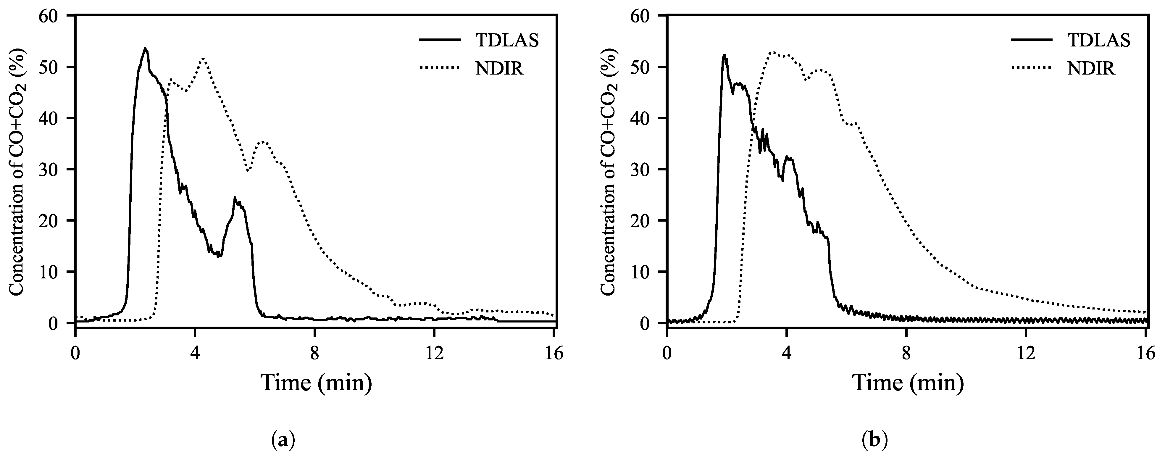
3.1. Comparison of Off-Gas Measurements Using TDLAS and NDIR Analyzers

Figure 3 shows the concentration of carbon oxides in the off-gas measured in real-time during the RH operations using TDLAS and NDIR analyzers during two representative RH operations. Here, the concentration of carbon oxides means the sum of CO and CO₂ concentrations. The change in the concentration of carbon oxides during the operations showed similar values and trends in both analyzers. However, the TDLAS analyzer was installed in situ closer to the vacuum chamber and due to its fast response characteristics, it was able to detect the changes in carbon oxide concentration about one minute faster than the NDIR analyzer. This shows that the TDLAS analyzer can measure the changes in the off-gas composition quickly and accurately in the RH process with high temperature and severe pressure changes.

Although the results of the measurements with the two types of analyzers showed similar trends overall, the graph of the measured values of the NDIR analyzer was wide and tended to decrease slowly toward the latter part of the operation. In general, the degassing reaction occurs intensively in the early stages of the operation and the reaction is significantly reduced after reaching a high vacuum [14,17,20]. Therefore, there should be a point at which the carbon oxide concentration in the off-gas converges rapidly to zero as in the graph measured by the TDLAS analyzer.

We assumed that one of the reasons why the measured value of the NDIR analyzer decreased very slowly in the latter of the operations was the reduced flow rate of the off-gas. Once the pressure is sufficiently low, the pressure in the vacuum chamber and the exhaust line is similar, reducing the overall off-gas flow rate and speed. Accordingly, at the end of the exhaust line, it takes a long time to detect the change in the off-gas composition occurring inside the vacuum chamber. Leakage in some of the long exhaust lines of the RH degassing unit due to equipment aging may also be another reason for the very slow decline of carbon oxide concentration measured by the NDIR analyzer late in the operations. On the other hand, by installing the TDLAS analyzers relatively close to the vacuum chamber, it was possible to reliably analyze the off-gas components regardless of the aforementioned reasons.

The carbon oxides gradually decrease after a sudden occurrence at the beginning of the RH operation, but in some operations, they tend to increase briefly in the middle of operation (about 5 min after the start of the operation in Figure 3a). This is called secondary decarburization. Although the exact cause is not known, we estimated that the gas components trapped in the molten steel were rapidly discharged as the circulating flow reached the maximum value. During this period, the flow rate of the off-gas increases and the pressure in the vacuum chamber is kept flat or decreases slowly.

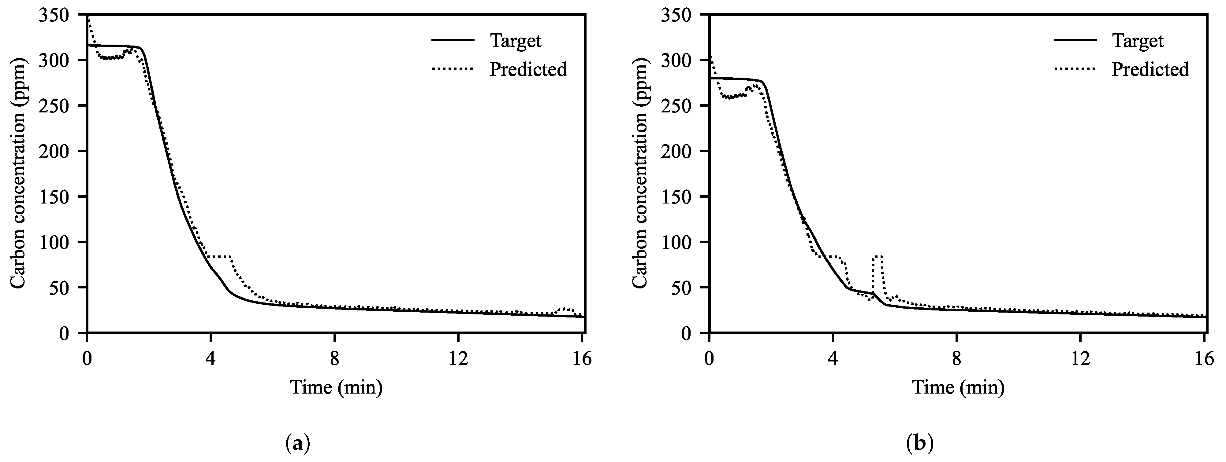
3.2. Verification of the Consistency of the Decarburization Curve

We compared the decarburization curves obtained using Equation (2) with the actual carbon concentrations measured through sampling in the molten steel (Figure 4). Three of the 12 operations used in the comparison were the cases in which carbon was added to the molten steel during the RH operation. We calculated the decarburization curves by using the measured values of the TDLAS and NDIR analyzer, respectively.

In the decarburization curves using the TDLAS analyzer, it was possible to confirm the point at which the decarburization rate changed rapidly. This is consistent with the results of previous studies [14,17,20] dividing the operation stage into two to three stages based on the period when the decarburization reaction changes rapidly in RH operation. On the other hand, it was difficult to clearly distinguish the stages of the decarburization reaction in the decarburization curve using the NDIR analyzer.

When carbon was not added during operation, Figure 4a shows that the decarburization curve using the TDLAS analyzer was similar to the actual amount of dissolved carbon, but the decarburization curve using the NDIR analyzer did not reflect the change in the actual values. From the results of Figure 3, we can deduce why the decarburization curve using the NDIR analyzer is different from the actual carbon concentration. It is difficult for the NDIR analyzer to immediately detect changes in the off-gas components emitted from the molten steel even if the decarburization reaction occurs intensely due to the installation location and its characteristics. In addition, even when the decarburization reaction decreases rapidly, the measured value of carbon oxides tends to decrease very slowly. Therefore, the decarburization curves obtained using the NDIR analyzer changed more slowly than the actual amount of dissolved carbon and showed relatively larger values than the actual values when the decarburization reaction was slow.

When carbon was added during the RH operations, Figure 4b showed that the decarburization curves differed from the actual amount of dissolved carbon. Additional carbon had been added about 3–4 min after the start of operation and the dissolved carbon content measured at about 6 min had increased. The difference in values was reasonable because we did not consider the effect of added carbon when calculating the decarburization curve. It is a meaningful task to identify changes in the decarburization curve due to the addition of carbon, but it is beyond the scope of this study. Instead, we used the weight of the added carbon as an input to the ANN model to train the effect of added carbon on endpoint carbon concentration.

Figure 5 shows the error between the predicted value of the decarburization curve using the TDLAS analyzer and the measured value of the carbon concentration in the molten steel for all the sampling values. At the early stage of the operations, the errors between the predicted value and the actual value were very large, but decreased rapidly as time passed. One of the reasons for the large prediction error in the early stages of the operations may be the difference between the sampling time of the molten steel and the recording time of the operation data. Since the decarburization reaction occurs very intensely in the early stages of operation, the carbon concentration may change significantly within a short time. Considering the manual sampling of the molten steel, even a small difference between the sampling time and the data recording time may increase the prediction error. In addition, the measured carbon concentration may vary depending on the sampling location because the molten steel is not uniformly mixed during this period [23,24,53]. However, in the latter stages of the operations, the decarburization reaction proceeds slowly and the uniformity of the molten steel is good due to the multiple circulation of the molten steel. Therefore, the influence of the sampling time and location is relatively small during this period. After 10 min from the start of the operations, the mean and standard deviation of the prediction error were small regardless of whether carbon was added during operation (

Table 1. Accuracy of the decarburization curves according to the carbon addition and operation time. The prediction error means the difference between the output of the decarburization curve and the actual amount of dissolved carbon obtained through sampling.

Processing Time	Error in Operations without Carbon Addition		Error in Operations with Carbon Addition
	Mean	Std. Dev.	Mean	Std. Dev.
<10 min	19.44 ppm	17.29 ppm	22.45 ppm	20.58 ppm
≥10 min	2.72 ppm	3.08 ppm	3.77 ppm	4.90 ppm

).

Since the decarburization curve obtained using the TDLAS analyzer explained the change of the actual carbon content in the molten steel well, we concluded that the decarburization curves could be used as a target value for supervised learning. Measuring dissolved carbon content over time is essential for creating a reliable, real-time prediction model. However, it is very hard to continuously obtain the dissolved carbon content that changes during operation due to time and cost limitations. This problem can be solved by using the output values of the decarburization curves as the actual carbon content. However, since the decarburization curve could be calculated after the end of operation, it cannot be used directly as an online model. Instead, we used the ANN model as a real-time prediction model of the dissolved carbon content.

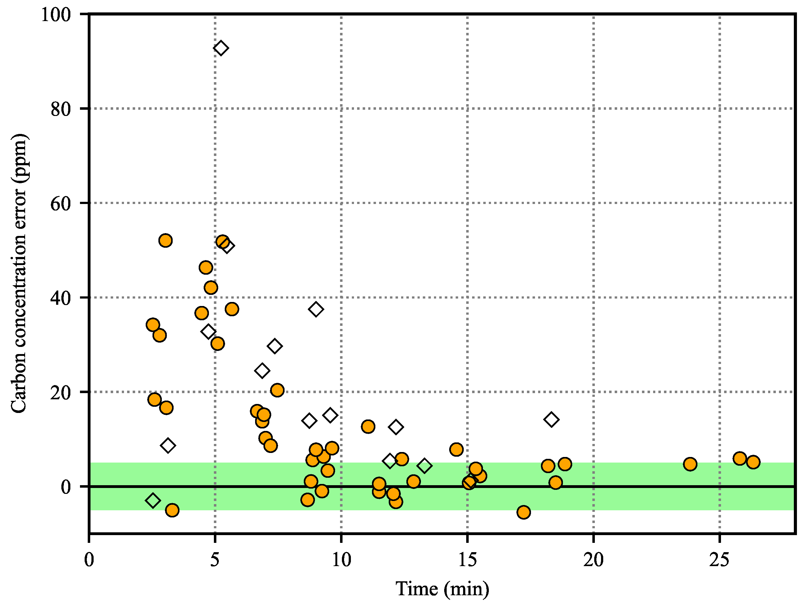
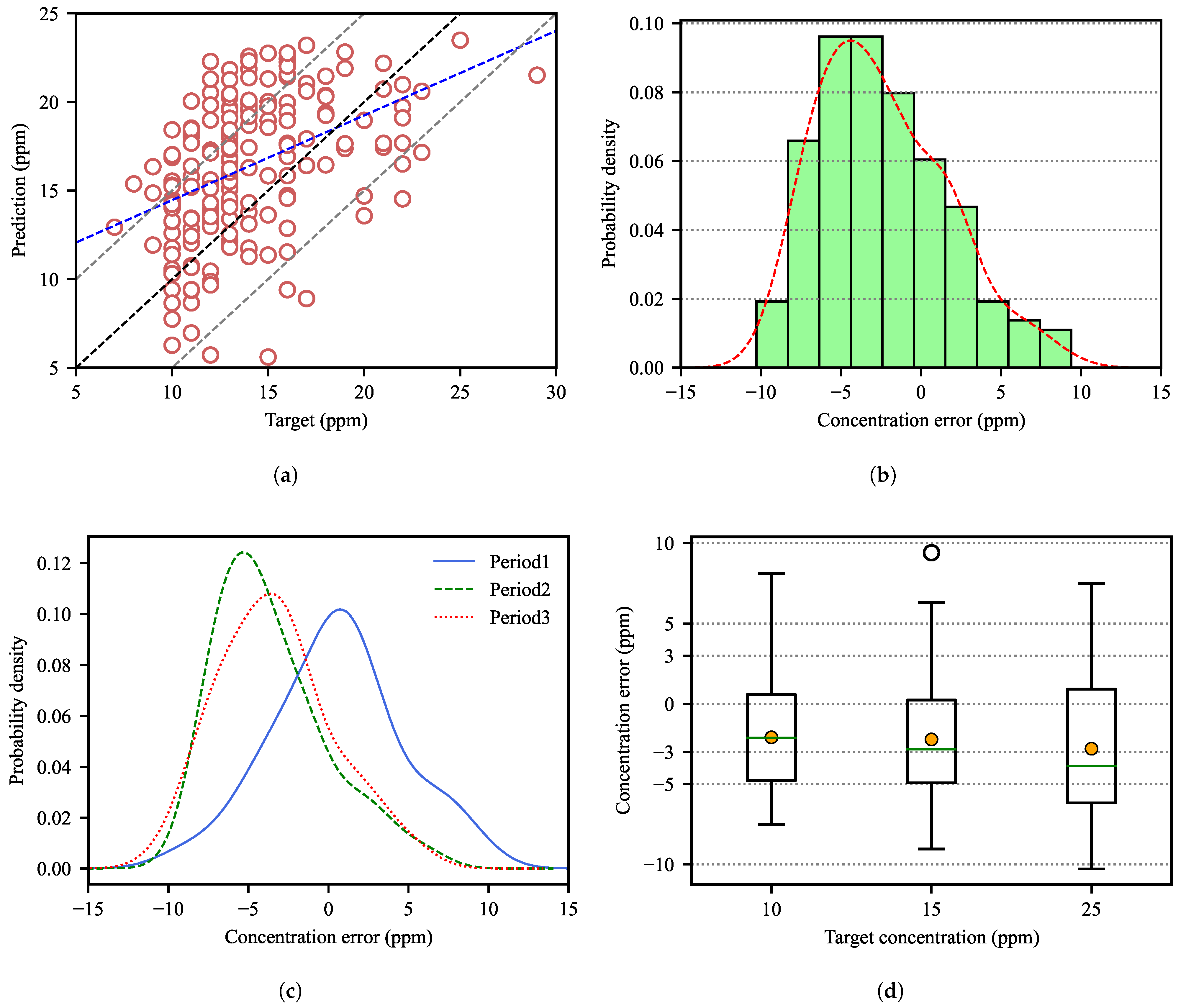
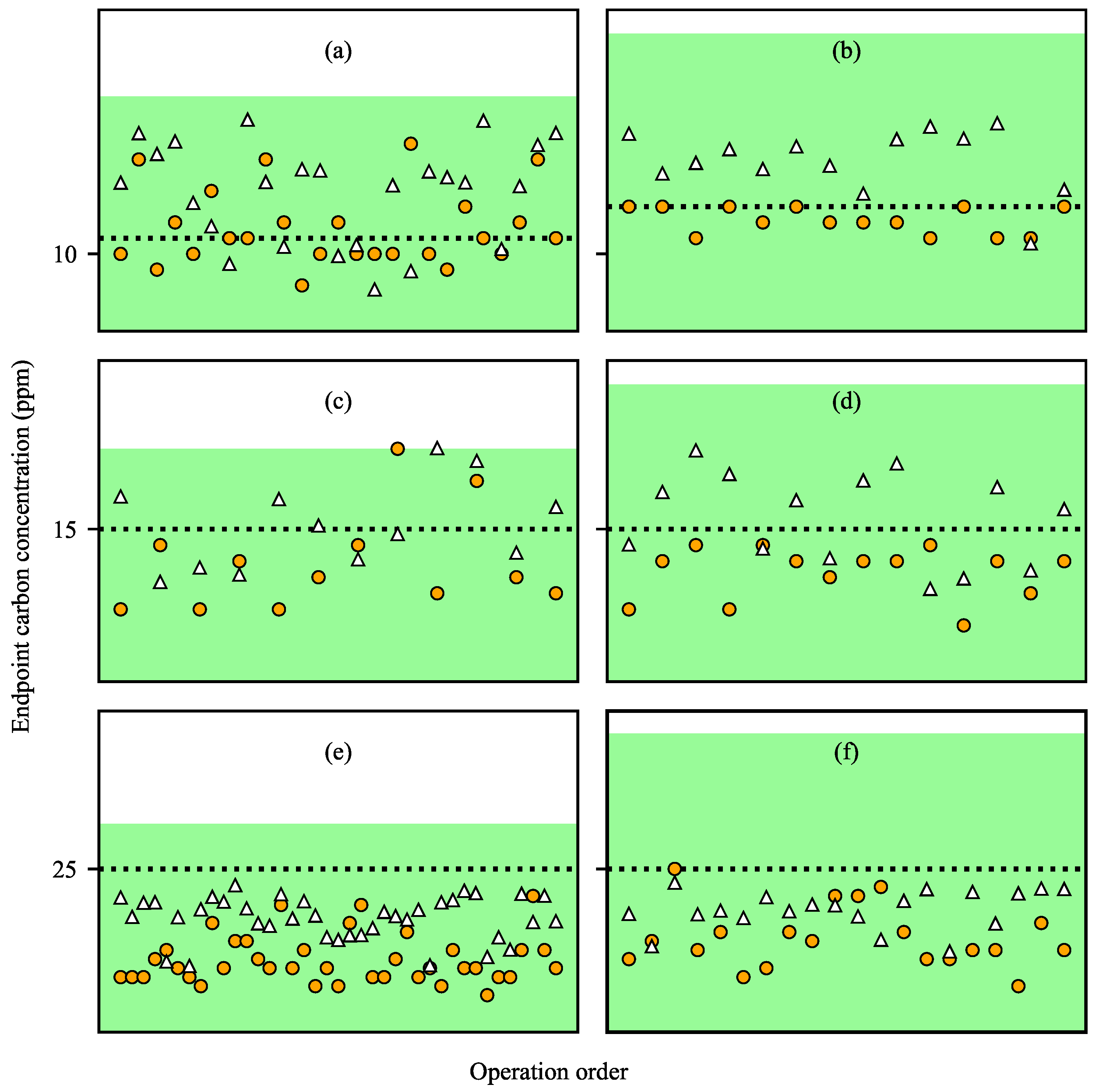
3.3. Predictive Performance of ANN Model

Contrary to initial expectations, excellent results were obtained with an RMSE of 18.6 ppm in a simple structure using one hidden layer with five neurons. When there were 10 and 15 neurons in one hidden layer, the RMSE was 73.6 ppm and 43.8 ppm, respectively, which gave poor results. The structure with three hidden layers showed the best results in the multilayer neural network (10-15-15); the RMSE was 17.9 ppm, which did not improved the performance significantly compared to the structure having one hidden layer.

Figure 6a,b shows the decarburization curves using the measured values of the TDLAS analyzer and the prediction results of the ANN model for them. Although the prediction results of the ANN model followed the decarburization curves well, the prediction values at the beginning of the operations were somewhat unstable. In particular, the initial values of the prediction curves often did not match the actual initial carbon concentrations already known from the measurements. A reason for this result was that we could not constrain the model so that the predicted value at the start of operation was the same as the actual initial carbon concentration. It will be possible to improve the predictive performance in the early stages of operations by training the model using data under various conditions. However, since this study focuses on the prediction of the endpoint carbon concentration, we leave it as a future challenge to improve the prediction performance in the early stages of operation.

At about 4 min after the start of operation, the predicted value of the ANN model showed a plateau, though the decarburization curve continued to decrease. Generally, the decarburization curves plateau when the second decarburization occurs (Figure 3a). The reason why the prediction error was relatively large around 4 min after the start of operation was because the model predicted that the secondary decarburization occurred during this period. The decarburization curve of Figure 6a shows no secondary decarburization and Figure 6b shows the occurrence of secondary decarburization in the short term. In order to accurately predict the secondary decarburization period, it seems that additional training using more diverse data is needed.

Interestingly, in Figure 6b, even though we did not consider the amount of added carbon when calculating the decarburization curves, some operations showed that the predicted values of the ANN model increased near the time of carbon addition. These results assumed that the predictive model had been trained to adjust the intermediate carbon concentration using the input information about the added carbon to follow the final carbon concentration.

Figure 7 shows the error distributions between the actual dissolved carbon concentration at the end of decarburization of the RH process and the predicted values of the prediction model for the test data.

In Figure 7a, the errors between the measured and predicted values of the endpoint carbon concentration were within ±10 ppm. The Pearson coefficient of correlation was 0.436, which means a moderate correlation between measured and predicted values. In general, it shows that the predicted value is larger than the actual measured values. Considering the measurement error of the actual concentration and the deviation between samples, the predictive performance was relatively good.

In Figure 7b, the distributions of prediction errors were right-skewed, which means that the actual dissolved carbon concentrations were somewhat smaller than the predicted values. This suggests that the ANN model was under-fitted due to the lack of data for various operating conditions, as there were many operations with similar initial carbon concentration and the molten steel weight. However, if we determine the decarburization end time using the predicted value, the actual carbon concentration is always below the upper target range of the concentration. Thus, it is possible to determine the decarburization end time for steels without a target lower limit.

Figure 7c shows the distribution of prediction errors according to the data collection period. In Period 1, the prediction error was evenly distributed around zero, but in Periods 2 and 3, it is right-skewed. There was facility maintenance work between Periods 1 and 2, so we estimated that changes in the facility and operating conditions might have affected the training of the prediction model. In particular, the circulation rate of the molten steel was increased due to facility improvement and as a result, the actual decarburization rate could be faster than Period 1 in the operation of Periods 2 and 3. Therefore, we expect that prediction accuracy will improve by iteratively training and upgrading the model by acquiring data that can reflect changes in facility and operating conditions.

Figure 7d shows the distribution of prediction errors according to the target carbon concentration. It was confirmed that the smaller the target carbon concentration, the smaller the prediction error and deviation (

Table 2. Prediction error of the ANN model according to the target carbon contents.

Prediction Error	Target Carbon Content
	10 ppm	15 ppm	25 ppm
Mean	−2.09 ppm	−2.22 ppm	−2.80 ppm
Std. dev.	3.56 ppm	3.96 ppm	4.47 ppm

). In general, the lower the target carbon concentration, the longer the operating time and the longer the slow decarburization reaction. In this case, the prediction error was small because the change in the carbon concentration in the molten steel was slow and the operating conditions were stable. On the other hand, if the target concentration is large, the operation is terminated when the variability in operating conditions and decarburization rate is relatively large. In this case, it seems necessary to train the model with more diverse data.

Figure 8 shows the predicted and measured values of carbon concentration for each steel type. In general, steels are classified into many types according to the target carbon concentration and the allowable concentration range. As discussed above, the predicted carbon concentrations in the molten steel were generally higher than the measured values, but both predicted and measured values were within the allowable concentration ranges. In particular, for the steel types of (b), (d), (e) and (f), both the predicted and measured values were much smaller than the upper limit of the allowable range, so it is possible to reduce the operating time using the predicted values and prevent excessive decarburization operations. For the steel types with small target values, the decarburization operations generally ended near the target values and excessive decarburization operations were rare. Therefore, it is necessary to further reduce the prediction errors in order to determine the accurate decarburization end time in these steel types.

Finally, the total prediction error of the ANN model for the test data was −2.43 ppm in the mean and 4.02 ppm in the standard deviation, which showed a good performance compared to previous studies [29,30].

4. Conclusions

The RH vacuum degasser is a very important secondary steelmaking process that determines the quality of the final product. In the RH process, it takes a lot of time to remove the carbon contents from the molten steel, so many studies have been conducted to reduce the decarburization time to improve productivity and reduce costs. In this paper, we proposed a method to accurately determine the decarburization endpoint by continuously predicting the dissolved carbon contents during the operation, which is difficult to measure directly. The decarburization curve, which continuously simulates changes in carbon content, was a novel approach to develop accurate online predictive models. By comparing the results of the real-time prediction model proposed in this study with the actual endpoint carbon contents, we obtained better prediction performance than previous studies. The total prediction error of the prediction model for the test data was −2.43 ppm in the mean and 4.02 ppm in the standard deviation, which was an excellent result compared to the other studies. Above all, we showed that the decarburization endpoint could be determined using the prediction model and the processing time could be reduced without affecting the final steel quality.

We expect that the methodology and real-time prediction model proposed in this paper can be widely used in predicting the components and temperatures required in various steel production processes. In addition, future challenges will involve improving the model to make it more suitable for steel production processes, using various algorithms such as Recurrent Neural Network (RNN) and Long Short-Term Memory (LSTM) with excellent time-series modeling performance.

References

1. Ghosh, A. Secondary Steelmaking: Principles and Applications; CRC Press: Boca Raton, FL, USA, 2000; pp. 147–185. [Google Scholar]
2. Stolte, G. Secondary Metallurgy: Fundamentals, Processes, Applications; Stahleisen: Dusseldorf, Germany, 2002; pp. 24–97. [Google Scholar]
3. Kor, G.J.W.; Glaws, P.C. Ladle refining and vacuum degassing. In The Making, Shaping and Treating of Steel; AISE Steel Foundation: Pittsburgh, PA, USA, 1998; pp. 661–713. [Google Scholar]
4. Zulhan, Z.; Schrade, C. Vacuum treatment of molten steel: RH (Rurhstahl Heraeus) versus VTD (vacuum tank degasser). In Proceedings of the 2014 SEAISI Conference and Exhibition, Kuala Lumpur, Malaysia, 26–29 May 2014. [Google Scholar]
5. Zhan, D.P.; Zhang, Y.P.; Jiang, Z.H.; Zhang, H.S. Model for Ruhrstahl–Heraeus (RH) decarburization process. J. Iron Steel Res. Int. 2018, 25, 409–416. [Google Scholar] [CrossRef]
6. Kuwabara, T.; Umezawa, K.; Mori, K.; Watanabe, H. Investigation of decarburization behavior in RH-reactor and its operation improvement. ISIJ Int. 1988, 28, 305–314. [Google Scholar] [CrossRef]
7. Schrade, C.; Huellen, M.; Zulhan, Z. New concepts for high-productivity RH plants. Metall. Res. Technol. 2006, 103, 445–451. [Google Scholar] [CrossRef]
8. Fukuda, Y.; Onoyama, S.; Imai, T.; Mukawa, S.; Sado, T.; Fukiage, K.; Kunitake, O.; Takagi, N.; Matsumoto, H. Development of high-grade steel manufacturing technology for mass production at Nagoya works. Nippon Steel Tech. Rep. 2013, 104, 90–96. [Google Scholar]
9. Baker, L.J.; Daniel, S.R.; Parker, J.D. Metallurgy and processing of ultralow carbon bake hardening steels. Mater. Sci. Technol. 2013, 18, 355–368. [Google Scholar] [CrossRef]
10. Hoshida, T.; Endou, G.; Ebisawa, T.; Taguchi, K.; Takahashi, K.; Kikuchi, Y. Melting of ultra-low carbon steel with RH. Tetsu-to-Hagane 1983, 69, S179. [Google Scholar]
11. Sumida, N.; Fujii, T.; Oguchi, Y.; Morishita, H.; Yoshimura, K.; Sudo, F. Production of ultra-low carbon steel by combined process of bottom-blown converter and RH degasser. Kawasaki Steel Tech. Rep. 1983, 8, 69–76. [Google Scholar]
12. Harashima, K.; Mizoguchi, S.; Kajioka, H. Kinetics of decaburization of low carbon liquid iron under reduced pressures. Tetsu-to-Hagane 1988, 74, 449–456. [Google Scholar] [CrossRef] [Green Version]
13. Kishimoto, Y.; Yamaguchi, K.; Sakuraya, T.; Fujii, T. Decarburization reaction in ultra-low carbon iron melt under reduced pressure. ISIJ Int. 1993, 33, 391–399. [Google Scholar] [CrossRef] [Green Version]
14. Higuchi, Y.; Ikenaga, H.; Shirota, Y. Effects of [C], [O] and pressure on RH vacuum decarburization. Tetsu-to-Hagane 1998, 84, 709–714. [Google Scholar] [CrossRef] [Green Version]
15. Han, C.; Ai, L.; Liu, B.; Zhang, J.; Bao, Y.; Cai, K. Decarburization mechanism of RH-MFB refining process. Int. J. Miner. Metall. Mater. 2006, 13, 218–221. [Google Scholar] [CrossRef]
16. Tavares, R.P.; Nascimento, A.A.; Pujatti, H.L.V. Mass transfer coefficients during steel decarburization in a RH degasser. Defect Diffus. Forum 2008, 273, 679–684. [Google Scholar]
17. Liu, B.S.; Zhu, G.S.; Li, H.X.; Li, B.H.; Cui, A.M. Decarburization rate of RH refining for ultra low carbon steel. Int. J. Miner. Metall. Mater. 2010, 17, 22–27. [Google Scholar] [CrossRef]
18. Tavares, R.P. Mass Transfer in Steelmaking Operations. In Mass Transfer in Multiphase Systems and its Applications; IntechOpen: London, UK, 2011; pp. 255–273. [Google Scholar]
19. Saint-Raymond, H.; Huin, D.; Stouvenot, F. Mechanisms and modeling of liquid steel decarburization below 10 ppm carbon. Mater. Trans. JIM 2000, 41, 17–21. [Google Scholar] [CrossRef]
20. Tembergen, D.; Teworte, R.; Robey, R. RH metallurgy. Millennium Steel 2008, 104–108. [Google Scholar]
21. Li, P.H.; Wu, Q.J.; Hu, W.H.; Ye, J.S. Mathematical simulation of behavior of carbon and oxygen in RH decarburization. J. Iron Steel Res. Int. 2015, 22, 63–67. [Google Scholar] [CrossRef]
22. Van Ende, M.A.; Kim, Y.M.; Cho, M.K.; Choi, J.; Jung, I.H. A kinetic model for the Ruhrstahl Heraeus (RH) degassing process. Metall. Mater. Trans. B 2011, 42, 477–489. [Google Scholar] [CrossRef]
23. Zhang, J.; Liu, L.; Zhao, X.; Lei, S.; Dong, Q. Mathematical model for decarburization process in RH refining process. ISIJ Int. 2014, 54, 1560–1569. [Google Scholar] [CrossRef] [Green Version]
24. Ling, H.; Zhang, L. A Mathematical model for prediction of carbon concentration during RH refining process. Metall. Mater. Trans. B 2018, 49, 2963–2968. [Google Scholar] [CrossRef]
25. Inoue, S.; Furuno, Y.; Usui, T.; Miyahara, S. Acceleration of decarburization in RH vacuum degassing process. ISIJ Int. 1992, 32, 120–125. [Google Scholar] [CrossRef] [Green Version]
26. Kim, B.I.; Choi, Y.J.; Park, S.Y.; Lee, J.S. The development of decarburization prediction model in RH process by Fuzzy logic technology. In Proceedings of the 2nd Asian Control Conference, Seoul, Korea, 22–25 July 1997; pp. 635–638. [Google Scholar]
27. Kim, B.I. The Development of Decarburization Ending Point Prediction Model Using Fuzzy Logic Technology in Secondary Refining Process. Master’s Thesis, Pohang University of Science and Technology (POSTECH), Pohang, Korea, 1997. [Google Scholar]
28. Kleimt, B.; Köhle, S.; Paura, G.; De Santis, M.; Granati, P.; Liberati, L.; Jungreithmeier, A.; Zuba, G. Improvement of Vacuum Circulation Plant Operation on the Basis of the BFI Simulation Model; EUR: Luxembourg, 2000.
29. Kleimt, B.; Köhle, S.; Jungreithmeier, A. Dynamic model for on-line observation of the current process state during RH degassing. Steel Res. Int. 2001, 72, 337–345. [Google Scholar] [CrossRef]
30. Zhang, G.F.; Chen, Y. Decarburization automatic prediction system in RH degasser. In Proceedings of the 2010 5th International Conference on Computer Science & Education (ICCSE), Hefei, China, 24–27 August 2010; pp. 986–989. [Google Scholar]
31. Jianwen, L.; Chengzhuang, L. Endpoint carbon content prediction of VOD using RBF neural network. In Proceedings of the 2013 2nd International Symposium on Instrumentation and Measurement, Sensor Network and Automation (IMSNA), Toronto, ON, Canada, 23–24 December 2013; pp. 588–590. [Google Scholar]
32. Rezaee, B. Desulfurization process using Takagi–Sugeno–Kang Fuzzy modeling. Int. J. Adv. Manuf. Technol. 2010, 46, 191–197. [Google Scholar] [CrossRef]
33. Chauhan, S.; Singh, M.; Meena, V.K. Comparative study of BOF steelmaking process based on ANFIS and GRNN model. Int. J. Eng. Innov. Technol. IJEIT 2013, 2, 198–202. [Google Scholar]
34. Wang, Z.; Liu, Q.; Liu, H.; Wei, S. A review of end-point carbon prediction for BOF steelmaking process. High Temp. Mater. Process. 2020, 39, 653–662. [Google Scholar] [CrossRef]
35. Meradi, H.; Bouhouche, S.; Lahreche, M. Prediction of bath temperature using neural networks. World Acad. Eng. Technol. 2008, 2, 946–950. [Google Scholar]
36. Yamaguchi, K.; Kishimoto, Y.; Sakuraya, T.; Fujii, T.; Aratani, M.; Nishikawa, H. Effect of refining conditions for ultra low carbon steel on decarburization reaction in RH degasser. ISIJ Int. 1992, 32, 126–135. [Google Scholar] [CrossRef]
37. Crawley, L.H. Application of Non-Dispersive Infrared (NDIR) Spectroscopy to the Measurement of Atmospheric Trace Gases. Master’s Thesis, University of Canterbury, Christchurch, New Zealand, 2008. [Google Scholar]
38. Hodgkinson, J.; Smith, R.; Ho, W.O.; Saffell, J.R.; Tatam, R.P. Non-dispersive infra-red (NDIR) measurement of carbon dioxide at 4.2 μm in a compact and optically efficient sensor. Sens. Actuators B Chem. 2013, 186, 580–588. [Google Scholar] [CrossRef]
39. Thomas, S.; Haider, N.S. A study on basics of a gas analyzer. Int. J. Adv. Res. Electr. Instrum. Eng. 2013, 2, 6016–6025. [Google Scholar]
40. Kazuto, T.; Tomoaki, N.; Yukihiko, T.; Junichi, M. TDLS200 tunable diode laser gas analyzer and its application to industrial process. Yokogawa Tech. Rep. English 2010, 53, 113–116. [Google Scholar]
41. Madabushi, J.; Fahle, D.; Heinlein, C. Calibration and validation philosophy and procedures for tunable diode laser analyzer in process applications. In Proceedings of the ISA 55th Analysis Division Symposium 2010, New Orleans, LA, USA, 25–29 April 2010. [Google Scholar]
42. Avetisov, V.; Bjoroey, O.; Wang, J.; Geiser, P.; Paulsen, K.G. Hydrogen sensor based on tunable diode laser absorption spectroscopy. Sensors 2019, 19, 5313. [Google Scholar] [CrossRef] [Green Version]
43. Kikkari, J.J. An Optical Process Sensor for Steel Furnace Pollution Control and Energy Efficiency. Master’s Thesis, University of Toronto, Toronto, ON, Canada, 2000. [Google Scholar]
44. Schlosser, E.; Ebert, V.; Williams, B.A.; Fleming, J.W.; Sheinson, R.S. NIR-diode laser based in situ measurement of molecular oxygen in full-scale fire suppression tests. In Proceedings of the 2000 Halon Options Technical Working Conference, Albuquerque, NM, USA, 2–4 May 2000; pp. 492–503. [Google Scholar]
45. Allemand, B.; Bockel-Macal, S.; Bruchet, P.; Januard, F.; Laurent, J. Continuous fumes monitoring for dynamic control of oxygen injections in EAF. In Proceedings of the 2nd International Conference On Process Development in Iron and Steelmaking, Scanmet II, Lulea, Sweden, 6–9 June 2004. [Google Scholar]
46. Januard, F.; Bockel-Macal, S.; Vuillermoz, J.C.; Laurent, J.; Lebrun, C. Dynamic control of fossil fuel injections in EAF through continuous fumes monitoring. Metall. Res. Technol. 2006, 103, 275–280. [Google Scholar] [CrossRef]
47. Lackner, M. Tunable diode laser absorption spectroscopy (TDLAS) in the process industries—A review. Rev. Chem. Eng. 2007, 23, 65–147. [Google Scholar] [CrossRef]
48. Krassnig, H.J.; Kleimt, B.; Voj, L.; Antrekowitsch, H. EAF post-combustion control by on-line laser-based off-gas measurement. Arch. Metall. Mater. 2008, 53, 455–462. [Google Scholar]
49. Tolazzi, D.; Marcuzzi, S.; Beorchia, S. LINDARC EAF off-gas analysis system-installation at Gerdau Ameristeel Jacksonville (Florida-USA). In Proceedings of the AisTech 2011, Indianapolis, IN, USA, 2–5 May 2011. [Google Scholar]
50. Arimoto, H.; Takeuchi, N.; Mukaihara, S.; Kimura, T.; Kano, R.; Ohira, T.; Kawashima, S.; Iwakura, K. Applicability of TDLAS gas detection technique to combustion control and emission monitoring under harsh environment. Int. J. Technol. 2011, 1, 1–9. [Google Scholar]
51. Brisson, D.; Grieshaber, K.W.; Sappey, A.D.; Chigwedu, C. Robust EAF laser gas analysis system-ZoloSCAN. In Proceedings of the AisTech 2014, Indianapolis, IN, USA, 5–8 May 2014. [Google Scholar]
52. Frish, M.B.; Laderer, M.C.; Smith, C.J.; Ehid, R.; Dallas, J. Cost-effective manufacturing of compact TDLAS sensors for hazardous area applications. Components Packag. Laser Syst. II 2016, 9730, 135–143. [Google Scholar]
53. Drozdz, P.; Falkus, J. The modeling of vacuum steel refining in the RH degassing unit based on thermodynamic analysis of the system. Arch. Metall. Mater. 2007, 52, 585–591. [Google Scholar]
Figure 1. Schematic diagram of the RH vacuum degasser.It shows the installation locations of the TDLAS and NDIR analyzers (filled circles).
Applsci 12 10753 g001
Figure 2. Input and output parameters of the ANN model. The target carbon contents are the result of the decarburization curve. The unit of the carbon content is parts per million (ppm), which means the weight fraction of carbon in molten steel.
Applsci 12 10753 g002
Figure 3. Changes in concentration of carbon oxides in the off-gas during two representative RH operations measured by TDLAS (solid lines) and NDIR (dotted lines) analyzers. Each graph represents the sum of the CO and CO2 concentrations measured at each time point. (a) Secondary decarburization is clearly shown. (b) Secondary decarburization did not occur.
Applsci 12 10753 g003
Figure 4. Comparison of the decarburization curves and the actual carbon concentrations (filled circles). Operations (a) without or (b) with additional carbon. The solid and dotted lines represent the decarburization curves obtained using TDLAS and NDIR analyzers, respectively.
Applsci 12 10753 g004
Figure 5. Prediction errors between the output of the decarburization curves using the TDLAS analyzer and the actual carbon concentrations. Empty diamonds and filled circles represent operations with or without additional carbon, respectively. A prediction is considered excellent if the prediction error is within ±5 ppm (green area).
Applsci 12 10753 g005
Figure 6. Prediction results of the ANN model for the target decarburization curves in two example operations (a) without and (b) with additional carbon. The solid and dotted lines represent the decarburization curve using the TDLAS analyzer and the predicted values of the ANN model, respectively.
Applsci 12 10753 g006
Figure 7. Predictive performance of endpoint carbon concentrations on test data. (a) Target vs. predicted values of the ANN model (blue line: regression line with slope 0.478; black line: ideal prediction line with slope 1.0; gray lines: the predicted values are within the ideal line ± 5 ppm); (b) error distribution for all test data; (c) error distribution by the period of collected data; (d) box plot of prediction error by target values (filled circles represent the mean values of each steel type).
Applsci 12 10753 g007
Figure 8. Measured (filled circles) and predicted (empty triangles) carbon concentrations at the end of decarburization by steel types. The target carbon content is: (a) 11 ppm, (b) 13 ppm, (c,d) 15 ppm and (e,f) 25 ppm. Areas filled in green indicate acceptable ranges of carbon concentrations and dashed black lines indicate target carbon concentrations. The X-axis of each plot represents the order of operation for each steel type.
Applsci 12 10753 g008