Abstract
In the calculus of functionally graded plates, the concept of multilayer plate is often used. For the use of this concept in this calculus, the continuous variation of the respective properties is replaced with a step variation. The first problem that arises in front of the user is related to the number of layers, which must be a finite and reasonably large number, to be accessible to the current calculus and to ensure the necessary accuracy of the results (under 5%). Another problem, generally poorly substantiated, is the one related to the assumption of a constant value of the Poisson’s ratio (usually 0.30 for the considered materials) over the entire plate thickness. The paper also contains a quantitative study of the influence of the Poisson ratio (4,…,10%), whose variation can be neglected, but only in certain circumstances. The presentation and substantiation of how to use the multilayer plate concept through models, methods and methodologies, along with the substantiation of the choice of the number of layers and the influence of the Poisson’s ratio, represent the main evidence of the originality of this work. The proposed numerical models are based on the use of common 3D finite elements. The software Ansys is used, which offers a multilayer finite element, which is taken into account in the comparative analysis of the results. The validation of the results is carried out by comparison with the analytical solution. The objective and purpose of this paper, that of completing the palette of achievements regarding the calculus of functionally graded plates, without modification of the stiffness matrices of the finite elements and using existing software products, are fulfilled.
1. Introduction
Functionally graded materials (FGMs) represent a special category of composite materials, usually made of two materials, with very different properties (Figure 1).
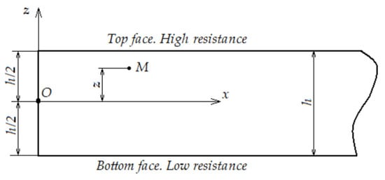
Figure 1.
The adopted coordinate system.
The material properties vary continuously (Figure 2) between the extreme surfaces of the material, where the properties are those of the respective materials in their pure state [1,2,3]. Today, the most used materials used in the construction of FGMs are ceramic materials and metals. Their volume fractions, in the thickness direction, varies continuously, according to a material law F(z), as Figure 2 shows.
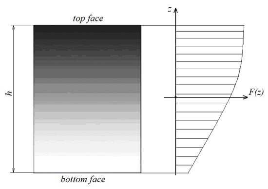
Figure 2.
The variation of the properties on the thickness of the material.
The material law function F(z) defines the variation of the elastic, physical and mechanical properties of the material (Young’s Modulus, Poisson’s ratio, density, thermal coefficient, etc.). Several material laws are known [3,4], having the names: Power Law, Reuss Law, Voigt Law, Local Representative Volume Element (LRVE) Law, Tamura Law, Mori-Tanaka Law, Exponential Law, Sigmoid Law and others. The best-known and most used material law, in practice and in the literature, is the Power Law (Sina et al., 2009), which for Young’s Modulus, F(z) ≡ E(z), has the expression [2],
where the indices “t” and “b” mean the top face or side of the material with higher properties, respectively the bottom face or side of the material with low properties and k is the power coefficient (values from ‘0’ to ‘∞’). In Figure 3, the variation of the material law function for E(z) is presented for different values of the power coefficient.
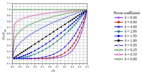
Figure 3.
Variation of material Power Law for different values of power coefficient k.
Of course, there are many other material pairs such as: polymer-elastomer, organic-inorganic glasses, etc. which can be used [4,5]. The name of such materials appeared in the mid-1980s, being introduced by scientific researchers from Japan, who were working on the creation of ultra-resistant materials at high temperatures for aerospace constructions.
The appearance of functionally graded materials attracted the attention of many scientific researchers [6,7,8,9,10,11], whose efforts were channeled in two directions: the realization (manufacturing) of these materials and the calculation of the structures from these materials. The two directions interfere and stimulate each other, especially in the field of materials design. In both directions the results are remarkable, but not finished; both manufacturing and calculation being in continuous development [12,13,14,15].
The field of use of FGMs [16,17] is very broad, such as biomedical equipment and instruments, medical prostheses, solar panels, aerospace constructions, sensor construction, optics, electronics and many others. The attention given to FGM is fully justified [18].
The present paper comes from the concern (purpose) to find models and calculation methodologies as simple as possible, as efficient as possible, based on the current knowledge of analytical and numerical analysis of structures [19], using widely accessible commercial analysis programs with the finite element method. In the field of calculation of plates from FGMs [20,21,22], the concept of multilayer plate is often used.
This concept is grounded in the calculus of functionally graded plates (FGPs), providing substantiated answers to a series of questions regarding the number of layers (their thickness), the influence of Poisson’s ratio, the influence of the power coefficient from the material law, etc. The calculation model and methodology, based on the concept of a multilayer plate, are validated by the calculus compared to the analytical solution of the plate bending rigidity, the maximum transverse displacement, the calculus of the stresses and the calculus of free vibration frequencies.
The results of the numerical calculation take into comparative analysis the use of the finite element dedicated to multilayer plates, from the library of the Ansys program [23]. The conclusions are based on quantitative determinations, on graphic representations, on comparative analyzes and the creation of models and practical methodologies, immediately applicable.
The purpose of our study is to make available to those interested in models, methods and methodologies for calculating of FGPs with existing and scientifically validated calculus means and procedures, without interventions in the classical theory of plates, without changes in the stiffness matrices of the finite elements, without building dedicated software products, without anything special, but solving a special problem, namely: the calculus of functional graded plates.
Nowadays, the literature on the calculus of functionally graded plates is rich one, but despite this fact, the calculus is mainly based on the determination of the bending rigidity of the plates by direct integration of the definition relation by neglecting the influence of Poisson’s ratio. The use of the multilayer plate concept, the use of their classical calculus relations [18], long validated theoretically and experimentally, allows us taking into account the influence of all calculus parameters.
The novelties of this study also consist in the theoretical substantiation of the use of the multilayer plate concept, in determining the influence of the adopted number of layers, in choosing their thickness and in developing a methodology for this purpose.
2. Multilayer Plate Concept
The plate is considered to be built by a number of layers, without slipping between them. Each layer is considered to be homogeneous and isotropic.
This concept of multilayer plate and its parameters are illustrated in Figure 4. For a plate, made up of a finite number of layers, each layer being considered homogeneous and isotropic, the bending rigidity D = D* is [24]:
where
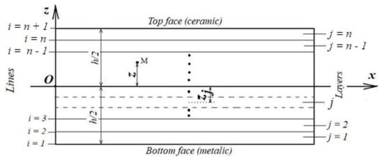
Figure 4.
The reference system, the lines “i” and layers “j” that define the multilayer plate.
The index j, in the relations (3) to (5) refers to the jth layer, like in Figure 4. So, the governing differential equation (Sophie-Germain) of the multilayered plates is [24,25]:
For a circular plane plate, with a constant distributed load pz the relation (3) becomes [24,25]:
The methodology for solving FGPs, based on the multilayer plate concept, involves replacing the continuous variation of the material properties (Figure 3), with a step variation (Figure 5), which would correspond to a set of 20 homogeneous and isotropic layers, each of them having different properties.
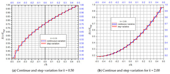
Figure 5.
The step variation, compared to the continuous variation at the layer level, for two values of power coefficient k.
Looking at the curves in Figure 5, we find that the step variation is not a constant one. This is higher or lower depending on the power coefficient value, which also influences the sign and value of the curvature.
3. Calculus of the FGPs Bending Rigidity
In the plate calculus, the determination of the bending rigidity (D) is of maximum importance, because the development of the calculation for the determination of any other parameters implies the knowledge of the bending rigidity.
3.1. The Multilayer Plate Method
The bending rigidity of the FGPs can be calculated using relations (2) to (5). This is an analytical solution, based on the concept of a multilayer plate.
3.2. Direct Integration Method
Another way of bending rigidity calculus is the direct integration [24,25] of the rigidity definition relation (8), with constant Poisson’s ratio:
When E(z) is replaced with relation (1), the solution of the relation (8) is:
4. Calcuus of the Material Density of FGPs
4.1. Analytical Calculus by Direct Integration
The plate equation of motion, [24,25], expressed in terms of bending and twisting efforts Mx, My, Mxy and displacement w(x,y,t) is written [26]:
where I0 is the inertial coefficient, having the following calculus relation:
Using the material Power Law also for density, the relation (11) is written:
Analytical solution of the integral (12) is:
The inertial coefficient I0 is the basis of the material density calculus, which for the case of a circular plane plate, takes place as follows:
4.2. Analytical Calculus by Multilayer Plate Concept
The methodology is similar to the one for calculating the Young’s modulus at the level of each layer (a constant value on the layer thickness), using the same material law:
5. Case Study
It is considered a plane circular plate, loaded with an uniformly distributed load, as Figure 6 shows, having the radius R of 50 [mm], the thickness h of 4 [mm] and the distributed load p of 5 [MPa].
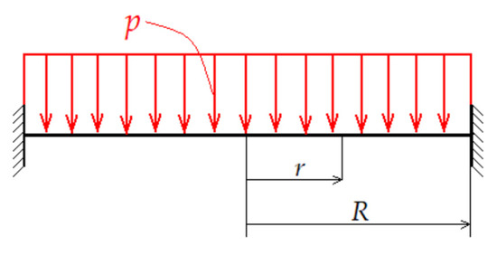
Figure 6.
Functionally graded circular plane plate.
The material properties are presented in Table 1.

Table 1.
Material properties.
5.1. Calculus of the Layer Material Properties
For a number of 20 layers, using for each layer, the z coordinate of its middle, using the relation (1) for Young’s modulus, relation (20) for Poisson ratio and relation (19) for material density, the values from Table 2 were determined.
Table 2.
Layer material properties for k = 0.05.
The same material law—Power Law—was used for all material parameters. The values presented in Table 2 are calculated for the value 0.05 of the power coefficient k.
The variation of these parameters on the FGP thickness is in steps; the variation curves are presented in Figure 7, for Young’s modulus and material density, respectively, for the same power coefficient k = 0.05. Poisson’s ratio has also the same variation, but often it is considered to have a constant value on the entire thickness.
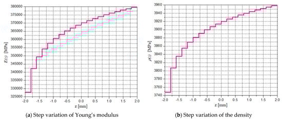
Figure 7.
Variation curves of some material properties, (a) Young’s modulus, (b) density.
From the analysis of Figure 5 and Figure 7, we find that for values of the power coefficient lower than one, the variation in steps is stronger in the part of the material with lower properties and vice versa.
In Table 3, the values of Young’s modulus are presented, for the FGP model, with 20 layers and different values of the power coefficient k, according to the methodology presented above, using the Power Law of the material properties variation.
Table 3.
The values of Young’s modulus E(zj) for different k values for 20 layers.
The values of the material properties, for any value of the power coefficient k and for any number of layers, can be known according to the presented methodology and used in the calculus of bending rigidity, displacements, stresses, free vibration frequencies, etc. regarding plates made of functionally graded materials.
5.2. Calculus of the Bending Rigidity of the Plate
The analytical calculation of the global stiffness of the FGP with relation (10) has the advantage that it does not use the concept of a multilayer plate but has the disadvantage that the Poisson coefficient value is considered constant.
The analytical calculation of the global stiffness of the FGP with relations (2) to (5) has the advantage that it can take into account the variation of Poisson’s ratio (in steps, as for all parameters of the FGP), but has the disadvantage that it has no connection with the number of layers.
Table 4 presents the values of bending rigidity for different values of Poisson’s ratio, as follows (in Table 4): ceramic material (νceram), average value of those two materials (νmed), average values depending on power coefficient k of the layer values (ν), constant value of 0.30 (νconst) and aluminum material (νalum).
Table 4.
The analytical values of bending rigidity by direct integration.
For the constant value of Poisson’s ratio, ν = 0.30, the following results presented in Table 5 were obtained, for the analytical calculus under concept of multilayered plate.
Table 5.
Layer number influence on bending rigidity.
Analyzing the results from Table 4 and Table 5, it is found that the bending rigidity of FGPs varies with the power coefficient k of the material law, with the number of layers (when using the concept of myltistrate plate) and with the Poisson’s ratio ν.
The graphic representations in Figure 8, in addition to the fact that they suggestively and correctly present the way of bending rigidity variation, allow us to find analytical variation curves, which can provide accurate data for any values of the parameters in the respective range.
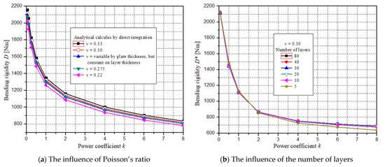
Figure 8.
Bending rigidity versus power coefficient k, for different Poisson’s ratio (a) and layers (b).
The curves in Figure 8 also show us that the bending rigidity value is slightly influenced by the Poisson’s ratio, Figure 8a and especially by the number of layers, Figure 8b. Moreover, in many works the influence of the Poisson’s ratio variation is neglected and a constant value of 0.30 is used. The mode of variation of the FGP bending rigidity versus the power coefficient k, calculated based on the concept of multilayer plate and on the analytical calculus by direct integration, is presented in Figure 9a. In Figure 9b, the errors between those curves are graphically presented.
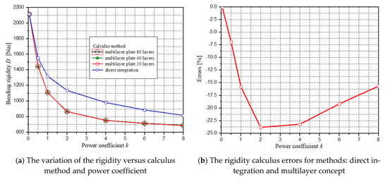
Figure 9.
Bending rigidity curves and their errors versus power coefficient k.
The use of the multilayer plate concept requires the adoption of a number of layers that ensure the necessary accuracy of all results. For this purpose, by comparing the bending rigidity variation curves depending on the number of layers with the analytical value, for different values of the power coefficient, the most suitable value of the number of layers is found. Such methodology is graphically presented in Figure 10a–f. The results coming from this methodology are comparatively presented in Table 6.
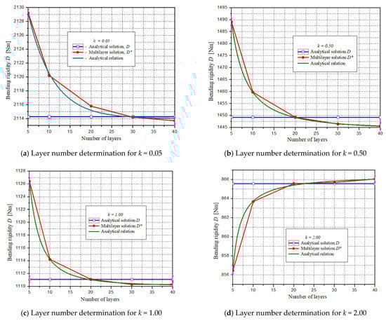
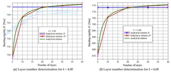
Figure 10.
Graphical determination of the layers number for some k values.
Table 6.
Analytical relations and their results.
Considering that the variation of the bending rigidity of the plate with the number of layers is represented on the basis of a small number of points (only 5), between which the variation is linear (a less credible case), we proceeded to find a mathematical relationship with non-linear variation, which will pass as close as possible, through the respective points.
The respective relationship allows us to find out the stiffness of the respective plate for any number of layers in the abscissa values range of the graph. This methodology applied to those 5 points where the plate rigidity was known, led to very close results, for which the calculus errors for 10 or more layers is below 1%, as seen in Table 6.
Looking at Figure 10, it can be seen that a number of 20 layers is the most suitable for using the multilayer plate concept, except for the case when for k = 0.05, the most suitable number is 30.
6. The Multilayer Plate Concept in the Numerical Calculus by FEM of FGPs
The multilayer plate concept can be used successfully, without changes in the theoretical foundations of the finite element method [27], with ordinary finite elements and with validated and widely accessible calculation programs.
In what follows, the Ansys program and the 3D finite element was used [28,29] in the available variants: ordinary structural finite element and multilayer finite element.
6.1. Finite Element Models
The numerical calculation by the finite element method was carried out using the 3D finite element Solid185 from the Ansys program library [28,29,30,31].
This finite element was used with two options: structural element (Figure 11a), which is a common finite element [31], implemented in many programs and multilayered finite element (Figure 11b), which is a special finite element, dedicated to multilayer structures (plates, beams, etc.).
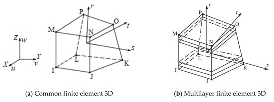
Figure 11.
Finite element 3D, Solid185 with its options (structural and layered).
Finite element model is presented in Figure 12. Because the structure—Figure 3—has two axes of symmetry [30,31] the finite element model is simplified one (quarter of structure), as it is presented in Figure 12a,b. In Figure 13, two details of the discretization are presented, referring to the finite element Solid185 with its options: structural element, respectively multilayer element (Figure 13b).
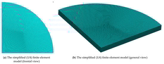
Figure 12.
The 3D finite element model for static analysis.
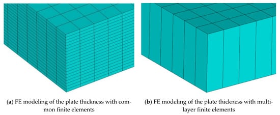
Figure 13.
FE mesh detail: (a) common FE, (b) multilayer FE.
As we can see looking at Figure 13b, when the multilayer finite element is used, the functionally graded plate is modeled with a single layer of finite elements.
In all the numerical calculus presented here, the multilayer plate concept was applied for a number of 20 layers. For each of the variants presented in Figure 13a,b, the material properties for each layer are entered—by different methodologies, according to the user manual [32].
In the analysis with FEM, we used a 3D model, with 3 dimensions of the finite elements: 1, 2 and 3 mm; the calculation model was a quarter of the structure, the plate having two axes of symmetry. The finite element models, for free vibration analysis is a complete model, as Figure 14 shows.
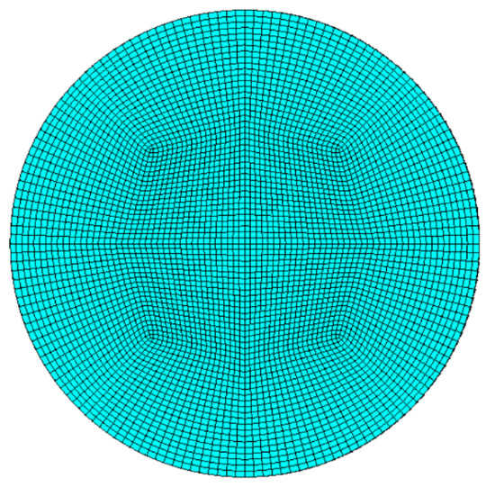
Figure 14.
The 3D finite element model for free vibration analysis.
6.2. Calculus of the Maximum Transverse Displacement
The calculus of the maximum transverse displacement (it occurs in the center of the plate) is calculated with the relation,
which leads to the following result:
The error between the values of and is only 0.07 percent. Practically, we can consider only one value of the analytical calculus, namely:
The results of the numerical calculus with finite elements, compared to the result of the analytical calculation, are presented in Table 7.
Table 7.
The values of the maximum transverse displacements.
The errors highlighted in the table validate both the application of the multilayer board concept and the methodology used. Using the common finite element (Model I) leads to even better results. than using the multilayer finite element (Model II), but it is more sensitive to the size of the finite element. The multilayer finite element is less sensitive [32] to the size of the finite elements. Figure 15 shows the field of transverse displacements of the functionally graded plate. Figure 15a refers to common finite element modeling, and Figure 15b refers to multilayer finite element modeling.
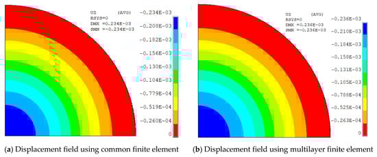
Figure 15.
Transversal displacements field of FGP.
The above results and errors show us the validity of the concepts, methods and methodologies used for problem solving. In all the details of the numerical calculation: the type of the finite element, its size, the choice of the number of layers, the correctness of the model, thus providing all useful information to any interested researcher, with access to the usual calculation means and procedures (not dedicated to structures made of functionally graded materials).
6.3. Calculus of the Stresses
Using the known relationships from plate theory, in clamped section, radial and tangential stresses are calculated with de relations:
The maximum values of the stresses occur at the level of the extreme faces (z = ±h/2). Since relations (23) and (24) are valid only for the homogeneous and isotropic plate, we will apply them to a fictitious homogeneous and isotropic plate, with the same bending stiffness, but with material characteristics available for entire plate thickness. This value of Young’s modulus is considered to be the average value (Table 2, column 3). Therefore:
Using relation (23) we obtain:
Table 8 presents in a comparative way, the results of the analytical calculus with the numerical one, based on the concept of multilayer plate. The errors regarding the result of the numerical calculation based on the multilayer board concept, compared to the result of the analytical calculation, validate the presented and used model and methodology.
Table 8.
The results of the stress calculus.
In Figure 16 and Figure 17 the stress fields σx ≡ σr (on the plate contour) are presented, by graphic post processing, on the deformed plate state.
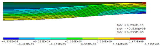
Figure 16.
Radial stress field on the contour, multilayered plate, common FE.
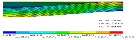
Figure 17.
Radial stress field on the contour, multilayered plate, multilayered FE.
In Figure 18, the variation of the radial stress on the thickness of the FGP is shown, in the clamped edges is presented. The variation is approximately linear, as it is known from general plate theory. As can be seen in Figure 18, in the middle of the plate, the stress is not zero, so the neutral plane is not positioned at the half of plate thickness. Additionally, the extreme stress values are not equal.
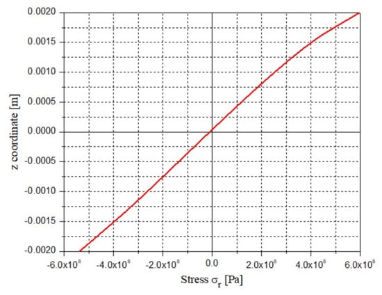
Figure 18.
Nodal radial stress variation on the plate thickness, in the clamped edges.
Using the relationships,
which come from the calculus model presented in Figure 19, the parameter d that defines the positioning of the neutral plane has the following calculus relation:
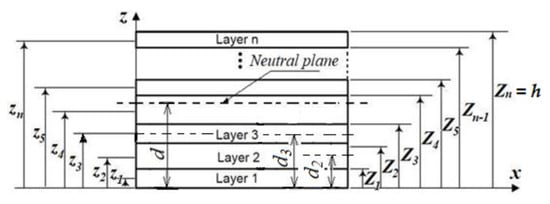
Figure 19.
Calculus model for determining the position of the neutral plane.
The position of the neutral plane can also be defined with respect to the median plane of the plate (the one that divides the thickness of the plate into two equal parts), by the parameter d*, defined by the relation:
The calculation of the two parameters, d and d* leads us to the results presented in the table below (Table 9), for the different values of the power coefficient k.
Table 9.
Neutral plane positioning parameters.
The graphical representation of the variation of the positioning parameter d versus the power coefficient k can be watched in Figure 20. We can notice that the shape of the curve presented in Figure 20 is similar to the shape of the variation curve of Young’s modulus versus power coefficient k (Figure 3).
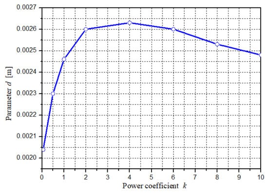
Figure 20.
Parameter d of the neutral plane positioning versus power coefficient k.
6.4. Calculus of the Free Vibration Frequencies
Analytically, we can determine the free vibration frequencies of thin circular plates [33,34] of homogeneous and isotropic material, by the relations (30) and (31).
In the relations (30) and (31), ωi is the vibration angular velocity “i” [rad/s], fi is the free vibration frequency “i” [Hz], R is the radius of the circular plate, h is the plate thickness and αi is a constant which depends on the number of nodal circles (S) and the number of nodal diameters (n), Figure 21, according to the data provided by the literature [33,34]. Some values of these parameters are presented in Table 10.
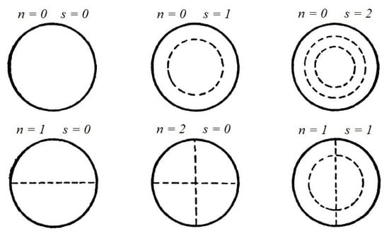
Figure 21.
Nodal circles and nodal diameters.
Table 10.
Some values of αi for some free vibration frequencies.
Using the concept of a multilayer plate, both for the analytical calculus and for the numerical one by FEM, we will use the average value of the density for those 20 layers (Table 2, column 10), denoted ρ* in bellow relation; the same observation is valid for the bending rigidity of the FGP (D*). So, the relation (30) is written:
The values of the parameters D* and ρ* from relation (32) are those calculated based on the concept of a multilayer plate (Table 5, column 4 and, respectively Table 2, column 10).
Table 11 shows the results of calculations based on the use of relations (30) and (31). Based on these results, the curves in Figure 22 were constructed. It can be seen that the free vibration frequency values decrease with increasing of the power coefficient values.
Table 11.
Some results of natural frequencies by analytical calculus.
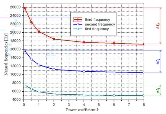
Figure 22.
Natural frequencies versus power coefficient k.
As Figure 22 shows, the rate of decrease in frequency with the coefficient k is the smallest for the first frequency, and the rate of decrease grows up with the number of frequencies (Δf3 > Δf2 > Δf1).
The numerical analysis with the finite element method of the free vibration frequencies was carried out in the same model variants, as in the previous cases. The results of the numerical analysis by FEM of the free vibrations for the considered FGP are presented synthetically, tabularly and graphically, in Table 12, respectively, by Figure 22. The values presented in Table 12 show that for first frequency, a very good concordance exists, regardless of calculus variants, compared to the analytical solution, based on the same concept of multilayered plate.
Table 12.
Some results regarding natural frequencies [Hz], by FEM calculated.
The analysis of the results in Table 12 and the graphs in Figure 23 shows that Model_I (ordinary finite element) lead to the results closest to the analytical calculus regarding the first three frequencies. The coincidence of the three curves is the best for the first frequency.
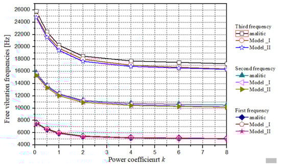
Figure 23.
Compared free vibration frequencies of analyzed FGP.
The shapes of the free vibration frequencies for those two models used (Model_I, Model_II) are presented in Figure 24, Figure 25 and Figure 26.
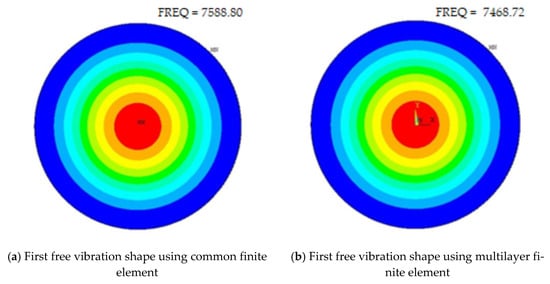
Figure 24.
The shape of the first frequency (n = 0; s = 0), Model_I (a) and Model_II (b)) frequency.
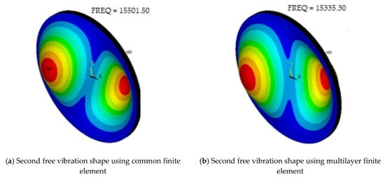
Figure 25.
The shape of the second frequency (n = 1; s = 0), Model_I (a) and Model_II (b).
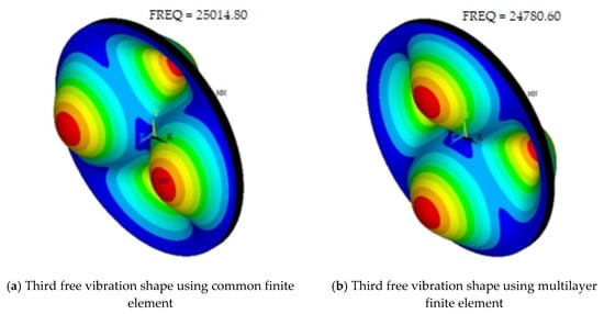
Figure 26.
The shape of the third (a) frequency (n = 2; s = 0), Model_I (a) and Model_II (b).
The errors, shown in Table 12, are graphically presented in Figure 27a for the first frequency and in Figure 27b for the second frequency. It can be immediately seen that Model_I lead to results closer to those calculated analytically.
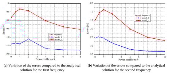
Figure 27.
Error variation between analytical and numerical results, versus power coefficient k.
7. Conclusions
This work is the fruit of our endeavors to find ways, means, models and methodologies for solving functionally graded plate calculation problems, with the currently available means, without interventions in the fundamentals of analytical or numerical methods, without the use of dedicated software products.
This being the objective of our research and of this paper, it meets our goal, that of making available to a large number of researchers an accessible, efficient calculus way, that complements the efforts and achievements of other researchers in this field.
The results of our research, some of which are presented in this paper, confirm the fact that the multilayer plate concept, proposed and used by us for the functionally graded plates calculus, proved not only valid, but very effective and suitable for solving of many problems. Among these, in this paper are detailed subjects such as the calculation of the bending rigidity, the calculus of the transversal displacements of the FGP, the calculus of the stresses, the calculus for determining the position of the neutral plane and the calculus of the frequencies of the free vibrations of the plate.
Certainly, other topics of the functionally graded plates calculus can be addressed, because any other calculus subject is based on the main parameters involved in the calculus of FGPs, illustrated in this paper. Regarding the rigidity calculus, an important choice that the researcher must make is whether to use direct integration—relation (9)—or the concept of a multilayer plate—relations (2)–(5). The results illustrated by Figure 9 show significantly different results, especially for values of the power coefficient greater than 1.
On the other hand, all calculus based on the determination of the bending rigidity with relations (2)–(5) lead to very close results, obtained both analytically and numerically. The cause of the inconsistency, between the FGP bending rigidity calculus by those two methods, is the hypothesis adopted according to which the Poisson’s ratio is constant throughout the thickness of the plate, a fact that allowed a facility for the mathematical calculus. In the multilayer plate concept, any parameter is considered constant, but only on the thickness of the respective layer. In our opinion, the influence of the variation on the plate thickness of the Poisson’s ratio is a weak one, but its complete neglect must be adopted with caution. This conclusion is based on the study carried out and illustrated in Figure 8. Therefore, for calculating the stiffness of FGPs, we recommend the multilayer plate concept.
Our research shows that the number of layers taken into account has a little influence, but only on the calculus of the global bending rigidity of the FGP, Figure 8b. Taking into account the variation of all the material characteristics on the plate thickness can be done successfully and without mathematical difficulties, only on the basis of the multilayer plate concept. The results can be significantly influenced, as can be seen from the analysis of the results in Table 4. This paper gives an original and substantiated answer regarding the choice of the number of layers, which leads to the desired accuracy. For the case study presented in this paper, the minimum number of layers is 20.
Applying this relationship (statistically determined) for the case study in this paper leads us to the number of layers used, namely 20 layers. We can recommend that the number of layers to result from the condition that the layer thickness to be less than or equal to the 20th part of the plate thickness expressed in meters.
The use, along with the usual finite element, of the multilayer finite element from the Ansys program library, allowed us an additional validation of the models and methodologies used to approach the calculus of FGPs based on the multilayer plate concept.
These conclusions, together with the conclusions and observations stated in the previous subsections, highlight the value and originality of our study regarding the use of the multilayer plate concept for the calculation of functionally graded plates.
The originality of this work is based on at least two strong points, namely: the use of the multilayer plate concept based on the classical theory, well known and verified and establishing a methodology for adopting a number of layers to ensure the desired accuracy.
Besides these, the use of the multilayer plate concept, which we recommend, allows taking into account all the calculus parameters, including the Poisson’s ratio, which is considered constant in the specialized literature. Regarding this aspect, the question arises as to what that constant value should be.
As seen in this work, through the results in Table 2 and Table 4 and Figure 8, the influence of Poisson’s ratio exists, it varies both with the power coefficient k, it can be highlighted both in analytical and numerical calculation and obviously, its influence depends on the values corresponding to the materials on the extreme faces.
An acceptable and accessible calculation, in terms of precision and calculation effort, taking into account any parameters that characterize the functionally graded plate, is currently represented by the use of the multilayer plate concept as presented in this paper.
All the conclusions of this study are supported by key quantitative values such as: the validity of the method, the model and the methodology through the error values from the comparative analysis of the results regarding the maximum transverse displacement of the plate (1.3%), the maximum radial stress in the plate (0.52%) and the calculation of the first frequency of the free vibrations of the plate (0.19%).
Besides these, we demonstrated (with the power of quantitative determinations) that the influence of the variation of the Poisson ratio is small, but not always negligible.
If the accuracy required for the calculation of a functionally graded plate also requires taking into consideration the variation of the Poisson’s ratio, the model, method and calculation methodology presented by us, based on the concept of a multilayer plate, represents a valid and accessible solution.
Funding
This research received no external funding.
Conflicts of Interest
The author declares no conflict of interest.
References
- Anju, M.; Subha, K. A Review on Functionally Graded Plates. Int. Res. J. Eng. Technol. 2018, 5. [Google Scholar]
- Toudehdehghan, A.; Lim, J.W.; Foo, K.E.; Ma’Arof, M.; Mathews, J. A Brief Review of Functionally Graded Materials. MATEC Web Conf. 2017, 131, 03010. [Google Scholar] [CrossRef]
- Pradhan, K.K.; Chakraverty, S. Overview of functionally graded materials. In Computational Structural Mechanics; Elsevier: Amsterdam, The Netherlands, 2019; pp. 1–10. [Google Scholar]
- Mahamood, R.M.; Akinlabi, E.T.; Shukla, M.; Pityana, S.L. Functionally graded material: An overview. In Proceedings of the World Congress on Engineering, London, UK, 4–6 July 2012; Volume 3. [Google Scholar]
- Marzavan, S. EFG Method in Numerical Analysis of Foam Materials. Mech. Time Depend. Mater. 2021, 26, 409–429. [Google Scholar] [CrossRef]
- Nastasescu, V.; Marzavan, S. An overview of functionally graded material models. In Proceedings of the Romanian Academy—Series A, Bucharest, Romania, 20 September 2022; Volume 23, pp. 257–265. [Google Scholar]
- Gilewski, W.; Pełczyński, J. Material-Oriented Shape Functions for FGM Plate Finite Element Formulation. Materials 2020, 13, 803. [Google Scholar] [CrossRef]
- Alshorbagy, A.E.; Eltaher, M.; Mahmoud, F. Free Vibration Characteristics of a Functionally Graded Beam by Finite Element Method. Appl. Math. Model. 2010, 35, 412–425. [Google Scholar] [CrossRef]
- Ramu, I.; Mohanty, S. Modal Analysis of Functionally Graded Material Plates Using Finite Element Method. Procedia Mater. Sci. 2014, 6, 460–467. [Google Scholar] [CrossRef]
- Kadoli, R.; Akhtar, K.; Ganesan, N. Static Analysis of Functionally Graded Beams Using Higher Order Shear Deformation Theory. Appl. Math. Model. 2008, 32, 2509–2525. [Google Scholar] [CrossRef]
- Yang, X.; Li, W.; Li, J.; Ma, T.; Guo, J. FEM Analysis of Temperature Distribution and Experimental Study of Microstructure Evolution in Friction Interface of GH4169 Superalloy. Mater. Des. 2015, 84, 133–143. [Google Scholar] [CrossRef]
- Chung, Y.-L.; Chen, W.-T. Bending Behavior of FGM-Coated and FGM-Undercoated Plates with Two Simply Supported Opposite Edges and Two Free Edges. Compos. Struct. 2007, 81, 157–167. [Google Scholar] [CrossRef]
- Huang, C.-S.; Lee, H.-T.; Li, P.-Y.; Chang, M.-J. Three-Dimensional Free Vibration Analyses of Preloaded Cracked Plates of Functionally Graded Materials via the MLS-Ritz Method. Materials 2021, 14, 7712. [Google Scholar] [CrossRef]
- Nguyen, D.K.; Bui, V.T. Dynamic Analysis of Functionally Graded Timoshenko Beams in Thermal Environment Using a Higher-Order Hierarchical Beam Element. Math. Probl. Eng. 2017, 2017, 1–12. [Google Scholar] [CrossRef]
- Hadji, L.; Bernard, F. Bending and Free Vibration Analysis of Functionally Graded Beams on Elastic Foundations with Analitical Validation. Adv. Mater. Res. 2020, 9, 63–98. [Google Scholar] [CrossRef]
- Tarlochan, F. Functionally Graded Material: A New Breed of Engineered Material. J. Appl. Mech. Eng. 2013, 2. [Google Scholar] [CrossRef]
- El-Galy, I.M.; Saleh, B.I.; Ahmed, M.H. Functionally Graded Materials Classifications and Development Trends from Industrial Point of View. SN Appl. Sci. 2019, 1, 1378. [Google Scholar] [CrossRef]
- Gupta, A.; Talha, M. Recent Development in Modeling and Analysis of Functionally Graded Materials and Structures. Prog. Aerosp. Sci. 2015, 79, 1–14. [Google Scholar] [CrossRef]
- Sebacher, B.; Hanea, R.G.; Marzavan, S. Conditioning the Probability Field of Facies to Facies Observations Using a Regularized Element-free Galerkin (EFG) Method. Pet. Geostat. Florence 2019, 2019, 1–5. [Google Scholar]
- Kapania, R.K.; Raciti, S. Recent Advances in Analysis of Laminated Beams and Plates, Part II: Vibrations and Wave Propagation. AIAA J. 1989, 27, 935–946. [Google Scholar] [CrossRef]
- Zenkour, A.M. Generalized Shear Deformation Theory for Bending Analysis of Functionally Graded Plates. Appl. Math. Model. 2006, 30, 67–84. [Google Scholar] [CrossRef]
- Singha, M.; Prakash, T.; Ganapathi, M. Finite Element Analysis of Functionally Graded Plates under Transverse Load. Finite Elem. Anal. Des. 2011, 47, 453–460. [Google Scholar] [CrossRef]
- Marzavan, S.; Sebacher, B. A new methodology based on finite element method (FEM) for generation of the probability field of rock types from subsurface. Arab. J. Geosci. 2021, 14, 843. [Google Scholar] [CrossRef]
- Szilard, R. Theories and Applications of Plate Analysis: Classical, Numerical and Engineering Methods. Appl. Mech. Rev. 2004, 57, B32–B33. [Google Scholar] [CrossRef]
- Timoshenko, S.; Woinowsky-Krieger, S. Theory of Plates and Shells; International Edition McGraw-Hill: New York, NY, USA, 1959. [Google Scholar]
- Chakraverty, S.; Pradhan, K.K. Vibration of Functionally Graded Beams and Plates; Academic Press: Cambridge, MA, USA; Elsevier: Amsterdam, The Netherlands, 2016. [Google Scholar]
- Marzavan, S.; Nastasescu, V. Displacement Calculus of the Functionally Graded Plates by Finite Element Method. Alex. Eng. J. 2022, 61, 12075–12090. [Google Scholar] [CrossRef]
- Bathe, K.J. Finite Element Procedures; Prentice-Hall, Inc.: Hoboken, NJ, USA, 1996. [Google Scholar]
- Huebner, K.H.; Dewhirst, D.L.; Smith, D.E.; Byrom, T.G. The Finite Element Method for Engineers, 3rd ed.; John Willey and Sons, Inc.: Hoboken, NJ, USA, 1995. [Google Scholar]
- Hughes, J.R.T. The Finite Element Method Linear Static and Dynamic Finite Element Analysis; Prentice Hall International Editions: Hoboken, NJ, USA, 1987. [Google Scholar]
- Zienkiewicz, O.C.; Taylor, R.L.; Zhu, J.Z. The Finite Element Method, 4th ed.; McGraw-Hill Book Company: New York, NY, USA, 2005. [Google Scholar]
- Kohnke, P. Theory Reference for the Mechanical APDL and Mechanical Applications; Release 12.0; ANSYS, Inc.: Canonsburg, PA, USA, 2009. [Google Scholar]
- Leissa, W.A. Vibration of Plates; National Aeronautics and Space Administration: Washington, DC, USA, 1969. [Google Scholar]
- Timoshenko, S. Vibration Problems in Engineering, 2nd ed.; D. Van Nostrand Company, Inc.: New York, NY, USA, 1937. [Google Scholar]


Publisher’s Note: MDPI stays neutral with regard to jurisdictional claims in published maps and institutional affiliations. |
© 2022 by the author. Licensee MDPI, Basel, Switzerland. This article is an open access article distributed under the terms and conditions of the Creative Commons Attribution (CC BY) license (https://creativecommons.org/licenses/by/4.0/).