Article

Model for Estimating the Modulus of Elasticity of Asphalt Layers Using Machine Learning

1
Faculty of Civil Engineering in Subotica, University of Novi Sad, Kozaračka 2a, 24000 Subotica, Serbia
2
Department of Civil Engineering and Geodesy, Faculty of Technical Sciences, University of Novi Sad, Trg Dositeja Obradovića 6, 21000 Novi Sad, Serbia
*
Author to whom correspondence should be addressed.
Appl. Sci. 2022, 12(20), 10536; https://doi.org/10.3390/app122010536
Submission received: 25 September 2022 / Revised: 15 October 2022 / Accepted: 16 October 2022 / Published: 19 October 2022
(This article belongs to the Section Civil Engineering)

Abstract

:
The management of roads, as well as their maintenance, calls for an adequate assessment of the load-bearing capacity of the pavement structure. This serves as the basis on which future maintenance requirements are planned and plays a significant role in determining whether the rehabilitation or reconstruction of the pavement structure is required. The stability of the pavement structure depends on a large number of parameters, and it is not possible to fully assess all of them when making an estimation. One of the most significant parameters is the modulus of elasticity of asphalt layers (EAC). The goal of this study is to use models based on machine learning to perform a quick and efficient assessment of the modulus of elasticity of asphalt layers, as well as to compare the formed models. The paper defines models for EAC estimation using machine learning, in which the input data include the measured deflections and the temperature of the upper surface of the asphalt layer. Analyses of modeling using artificial neural networks (ANNs), support vector machines (SVMs) and boosted regression trees (BRT) were compared. The SVM method showed a higher accuracy in estimating the EAC modulus, with a mean absolute percentage error (MAPE) of 7.64%, while the ANN method and the BRT achieved accuracies of 9.13% and 8.84%, respectively. Models formed in this way can be practically implemented in the management and maintenance of roads. They enable an adequate assessment of the remaining load-bearing capacity and the level of reliability of the pavement structure using non-destructive methods, at the same time reducing the financial costs.

1. Introduction

Pavement constructions of highways, main roads and local roads are most often realized as flexible pavement constructions. Due to the negative impact of traffic load, various weather conditions and other parameters on the load-bearing capacity of pavement structures, it is necessary to implement a maintenance program in order to determine when and where maintenance works need to be carried out.
Non-destructive methods and the backcalculating method of the elasticity of asphalt layers (EAC) have proven to be reliable when it comes to analyzing the mechanical properties of the pavement structure, and therefore can be used for the assessment of the load-bearing capacity of pavement structures and their remaining service life [1,2,3,4,5,6].
A non-destructive method provides a mechanical approach to pavement design. In this paper, deflection data were obtained by a non-destructive method using a falling weight deflectometer (FWD) device. For the data obtained in this way, backcalculation procedures were used to determine the stiffness of the individual layers of the pavement structure. In order to calculate the modules as accurately as possible, it was necessary to measure the deflections at different locations along the road section, all of which featured a uniform layer thickness.
Currently, there are a number of models for calculating the modulus of elasticity. The two basic divisions of modeling methods include classical methods and methods based on artificial intelligence. Artificial intelligence has wide applications in different areas of construction. The most frequently applied artificial intelligence method, which has proven to be a successful alternative for predicting the elasticity modulus from deflection data, is machine learning (ML). Machine learning methods are defined by systems that solve complex problems for which there are no sequential algorithms, but only data about solutions. Based on such data, these methods form their own solutions according to their own learning rules. ML methods are successfully applied in order to solve complicated problems in construction [7,8], and they have also proven to be a highly efficient problem-solving tool when applied in civil engineering [9,10,11,12]. The ML methods used in this paper involve artificial neural networks (ANNs), support vector machines (SVMs) and boosted regression trees (BRTs).
As a result of the shortcomings of classical calculation and the complexity of inverse modeling, numerous calculations have been developed and implemented. These range from the simplest programs to advanced methodologies based on artificial intelligence. There has been an increasing application of computational methods based on artificial intelligence, since they are aimed at reducing the sensitivity of calculation results and errors that occur during measurements [13].
Neural networks and genetic algorithms can be applied to optimize backcalculated moduli, in order to avoid premature convergence and to obtain reliable elastic moduli [14,15].
According to some research [16,17,18], in order to obtain the most realistic properties of the pavement construction through neural networks modeling, it is necessary to apply a synthetic database of measured deflections. However, to perform such a calculation, the measured deflections and the thickness of the pavement structure layers, as well as Poisson’s coefficient, need to be entered as the input parameters.
Recent research studies by Gopalakrishnan [19,20] have focused on the development of flexible pavement analysis models based on neural networks which are trained using finite elements for predicting critical pavement responses and layer moduli.
By using the ANN method, Baldo et al. [21,22] predicted the modulus of elasticity of the asphalt layers of airport pavement structures. The deflections, on which the formed models of homogeneous sections were based, were measured by a heavy weight deflectometer. The results were compared depending on the combination of input parameters (deflections, layer thickness and coordinates of the corresponding homogeneous section) and the combination of activation functions. Saltan and Terzi [23] created a model using the ANN method for predicting the elasticity modulus of asphalt layers and their thickness, using the input parameters of deflections measured by the FWD device.
Gopalakrishnan [24] predicted the elasticity modulus of the asphalt layer and the lower load-bearing layers using the SVM method. The input parameters for the asphalt layer moduli included layer thickness and measured deflections, whereas the lower load-bearing layer input parameters included the obtained asphalt layer moduli, layer thicknesses and measured deflections. The results were compared with the models created by the ANN method. Subsequently, a conclusion was drawn that the SVM method can represent an alternative to the ANN method, keeping in mind that the required database is often limiting and unrepresentative.
Saltan [25] wrote the first research paper based on ML, in which models were designed with multiple methods, including ANNs, SVMs and BRTs. He predicted the modulus of elasticity and Poisson’s coefficient with the input parameters of the measured deflections.
In this work, the models were created within the aforementioned ML methods. Moreover, the impact of the input data on the output values of the EAC model was analyzed. Owing to possible problems while collecting data for input parameters, one of the main aims of this research is the automation of backcalculation procedures while reducing the number of input parameters needed for calculations, so as to obtain reliable and sufficiently accurate EAC values in a more rapid way. The research aims to find the best forecasting model, which would be much more practical to apply.

2. Theory and Calculation

The ANN [26] method requires a large set of data for network training. It then quickly calculates the required output data with significant accuracy and precision, in comparison with classical methods and neuro-fuzzy systems [27]. The SVM method has been derived from the statistical theory of learning [28], which applies structural risk minimization, while the ANN only applies the minimization of the mean square error in the data set. As a result, a better prediction is obtained by the SVM model. The BRT [29] method is a supervised learning method that contrasts with ANN and SVM. Other methods process ML data numerically and result in one “best” model. However, the BRT theory processes them independently of their assumptions and uses the boosting method to combine a large number of relatively simple models for the optimization of predictive performance.

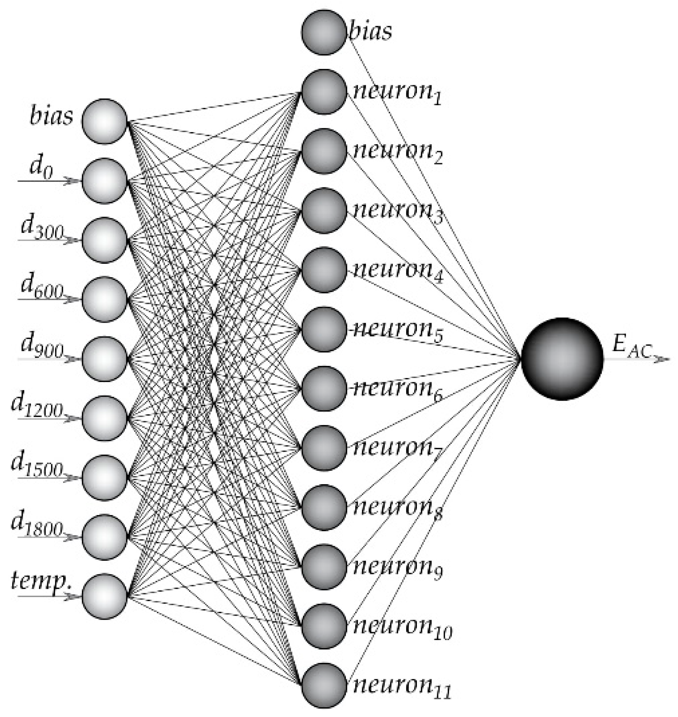
2.1. Artificial Neural Networks (ANN)

An ANN is a machine-learning method used for evaluating and processing of information. The general structure of an ANN consists of an input layer, one or more hidden layers and an output layer.
The formation of an ANN model undergoes three phases: the network modeling phase, network training phase and performance evaluation phase.
To define the network architecture, a range of parameters are used, such as:
  • number of input parameters;
  • number of layers and neurons in them;
  • number of output data;
  • selection of activation functions of hidden and output neurons;
  • type of training function, whether the network is forward- or backward-oriented.
In this paper, the available data set is divided into training data, validation data and testing data. In the training phase, the model is trained with the learning algorithm Levenberg–Marquardt (LM), a second-order numerical optimization technique which combines the advantages of the Gauss–Newton and the steepest descent algorithms. It is very effective when training networks that have up to several hundred units of weight [30].
Supervised learning involves two basic steps, a forward and a backward one. Neural network training incorporates the following steps for the fine-tuning of weights and biases, in order to obtain the most accurate solutions at the output [26,31]:
Step 1: Model initialization: initializes weights and biases;
Step 2: Forward propagation: using the given input xi, weights wi and biases b, the linear combination of inputs and weights (zi) is calculated for each layer. After that, the output values (ai) are calculated by applying the activation function to (zi), represented in the Equation (1):
a i = f ( z i ) = f ( j = 1 R x j w i , j + b )
In the current study, the logistic sigmoid (LogS) was used for the hidden activation function, while the output layer was associated with the linear activation function (purelin) [32]. Activation functions and expressions are shown in Figure 1.
Step 3: Compute the loss function, based on which the difference between the obtained prediction and the given target values is reached. The calculation is based on the mean square error, represented in Equation (2):
M S E = 1 n 1 n ( y i a i ) 2
Step 4: Backpropagation is conducted, in which the gradients of the loss function are calculated. Using these gradients, the parameters are adjusted from the last layer to the first one.
Step 5: Iterations are repeated until it is observed that the loss function has been minimized, without overfitting the training data.
The described process of the feed-forward neural network and backpropagation is schematically shown in Figure 2.
In this paper, the input neurons include the measured deflections and surface temperature of the asphalt layer. The best ANN architecture for the EAC prediction comprises eight input neurons, one hidden layer with eleven neurons and one output neuron (Figure 3).
The learning rate and adaptation parameter Mu affect the convergence speed of the backpropagation algorithm. A learning rate of 0.001 and an adaptation parameter Mu of 0.001 were chosen. The epoch (iteration number) was limited to 1000 during training. The database for ANN modeling is divided in the following way: 85% for the training set, 10% for the validation set and 5% for the testing set.

2.2. Support Vector Machine (SVM)

A SVM is a machine-learning method often applied for classification and regression, and it was first identified by Vapnik. SVM regression is considered a non-parametric method since it relies on kernel functions.
In training data set   { ( x 1 , y 1 ) ,   ( x 1 , y 1 ) , ,   ( x l , y l ) } Χ   x   R , Χ denotes the space of the input data x of n-dimensional vectors. SVM uses f ( x , w ) = i = 1 N w i · φ i ( x ) as an approximating function. The function f ( x , w ) is explicitly written as the function of weights w, which are the subject of the training.
The evaluation of the regression model based on the SVM rests upon the evaluation of the approximation error, which tolerates errors within the ε-insensitivity zone. There is also the possibility of displaying the error outside of the ε-insensitivity zone, by introducing the linear loss function, represented in Equation (3) [28,33]:
| y f ( x , w ) | ε = { 0 | y f ( x , w ) | ε   i f i f | y f ( x , w ) | ε | y f ( x , w ) | > ε
The main goal of the SVM algorithm is to simultaneously perform the minimization of R e m p ε and   w . The linear regression hyperplane f ( x , w ) = w T x + b is obtained by minimizing the actual error, as given in Equation (4):
R = 1 2 w 2 + C ( i = 1 l | y i f ( x i , w ) | ε )
If slack variables ξ and ξ * for the deviations above and below ε tube are introduced (Figure 4), in order to overcome the impossible limitations of the optimization problem, the expression stated in Cortes and Vapnik is obtained. It is represented in Equations (5) and (6) [28]:
R w , ξ , ξ * = [ 1 2 w 2 + C ( i = 1 l ξ + i = 1 l ξ * ) ]
subject   to   { y i w T x i b   ε + ξ , i = 1 , l w T x i + b y i   ε + ξ * , i = 1 , l ξ , ξ *   0 , i = 1 , l  
The constant C > 0 is a pre-determined tolerance parameter which penalizes errors (large values of ξ and   ξ * ) that are greater than ε, thus reducing the approximation error.
The optimal hyperplane is obtained by maximizing the dual Lagrange function. After solving the dual regression problem, the following parameters are obtained:
  • optimal weight vector: w o = i = 1 l ( α i * α i ) x i
  • optimal bias: b o = 1 l i = 1 l ( y i x i T w o )
which define the optimal regression hyperplane, represented in Equation (7):
f ( x , w ) = w T x + b
where α i * ,     α i are Lagrange multipliers.
A kernel function is used to approximate a non-linear function. Vectors x i are transferred into the multi-dimensional space through the mapping Φ   :   Χ   where (z-space) represents the future space. The final approximate function is defined by the following expression as given in Equation (8):
f ( x ) = i = 1 l ( α i * α i ) K ( x i , x j ) + b
In this paper, the Gaussian (RBF) kernel function was used, defined by the following expression, represented in Equation (9):
K ( x i , x j ) = e x p ( 1 2 σ 2 x x i 2 )
where σ is the width of the RBF function.
The SVM algorithm was tested with different parameters for the ε precision parameter, C tolerance parameter and kernel scale factor γ . The best results for SVM modeling were obtained with the algorithm parameters shown in Table 1.

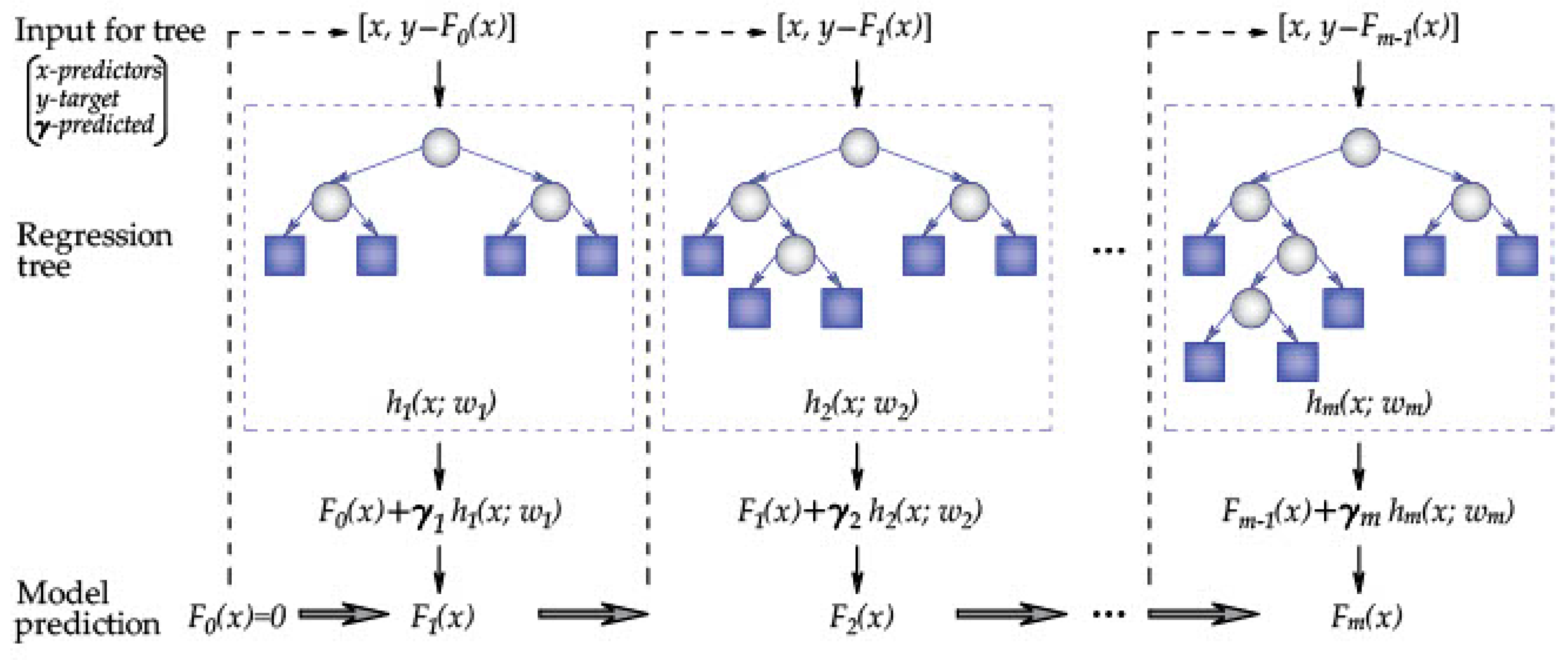
2.3. Boosted Regression Tree (BRT)

Gradient boosting (GB) is one of the machine learning methods used to solve classification and regression problems, and was developed by Jerome Friedman [34]. The GB algorithm is an optimized algorithm based on the error function. Decision trees form strong prediction models, which are created by merging base prediction models. GB is a method in which a decision tree is repeatedly added so that the next decision tree corrects the error of the previous one. The gradient optimization method is based on adjusting the last result by adding a negative value of the gradient of the function which is to be minimized. Hence, by constantly adjusting the weight of a base learner, it makes it a stronger learner. A schematic diagram of BRT is shown in Figure 5 for demonstration.
The least-squares boosting (LS Boost) algorithm is an approximation of the function Fm-1, which minimizes the expected value xi, of some specified loss function. The calculation of loss function is based on the mean square error, represented in Equation (10):
L ( y i ,   F ( x i ) ) = 1 n i = 1 N ( y i F m 1 ( x i ) ) 2
The BRT model and boosting regression tree h m ( x ; w ) are formed as follows [34,35]:
Step 1: Model initialization, represented in Equation (11):
F 0 ( x ) = argmin γ i = 1 N L ( y i , γ )
Step 2: Iterative procedure of obtaining M regression trees:
(1)
The negative value of the gradient of the loss function L ( y i ,   F ( x i ) ) is calculated, and then it is used as the estimate of the residual, as given in Equation (12):
y ˜ i = [ L ( y i , F ( x i ) ) F ( x i ) ] F ( x ) = F m 1 ( x )
(2)
A regression tree h m ( x ; w ) is optimized for the residual obtained in the previous iteration. The step size of the gradient drop is calculated, as represented in Equation (13):
( γ m , w m ) = argmin γ , w i = 1 N [ y ˜ i γ h ( x i , w m ) ] 2
Step 3: An approximation update is performed, represented in Equation (14):
F m ( x ) = F m 1 ( x ) + ν γ m h m ( x , w m )
where ν represents the learning rate, which prevents the over-fitting of the model.
The LS Boost algorithm was tested with different parameters for the learning rate, number of boosting stages and leaf size. The best results for BRT modeling were obtained with the algorithm parameters shown in Table 2.

3. Dataset

Based on the measured deflections, the EAC are obtained through backcalculation procedures. Classical backcalculation procedures require the assumption of the initial modulus of elasticity at the beginning of the calculation, on which the convergence further depends. A wrong choice of the initial modulus of elasticity often leads to a calculation that is not sufficiently accurate. Other problems that affect the accuracy of the calculation include the accuracy of measurements, the number and thickness of the pavement construction layers, as well as the temperature of the asphalt layers [36,37,38,39].
In order to form a model for predicting the elastic modulus of asphalt layers of flexible pavement structures, it is necessary to form a set of data of the measured deflections and temperature, which contain a sufficient amount of information. Based on this data set, the modulus of elasticity is calculated using classic backcalculation procedures.
Starting from the defined goals and the analysis of the research plan and program, a database that first needs to be thoroughly examined and processed is chosen. Data analysis and processing mean that when deflections are measured on the primary and secondary roads and highways, the recurring points that represent extremes and significant deviations are removed. In this way, they do not affect the data analysis. In addition, 462 pieces of information were collected for analysis, 438 of which were taken for network training, which amounts to 95% of the total amount of data. Network testing was performed based on 23 pieces of information, which is 5% of the total amount of data. The statistics of the data used in the modeling are shown in Table 3.
The models were modeled by the ANN, SVM and BRT methods using the MATLAB software package. The input variables are deflections d0, d300, d600, d900, d1200, d1500, d1800, i.e., the measured deformations at vertical distances of 0, 300, 600, 900, 1200, 1500, 1800 mm from the center of the loading plate and the temperature of the upper surface of the asphalt layer. The deflections were mostly measured in spring and autumn in the early morning hours, except for one section on the highway, which was measured in the summer period in the morning hours. ELMOD 6 software was used for the backcalculation. Three methods for calculating the asphalt modulus can be selected in this software. They include the finite element method, linear elastic theory and method of equivalent thicknesses. In this paper, the linear elastic theory was used. Since in the Republic of Serbia there is no recommendation for using these three methods, British standards are used [40]. The output variable is the modulus of elasticity of the asphalt layers (EAC) expressed in MPa.
The deflections were measured based on the load which ranges between 48.63 and 50.89 kN. Due to such a small range, the load is considered constant, and hence it is not taken as an input variable. The thickness of asphalt layers was measured at intervals of 1 km and for that reason was not taken as an input variable.
According to British standards [40], the bearing capacity of the structure is divided into three sections, according to the module values:
  • modules up to 3000 MPa—poor bearing capacity overall;
  • modules from 3000 MPa to 7000 MPa—there are damages in some places;
  • modules above 7000 MPa—good bearing capacity overall.
As a result of the aforementioned division, in this research, the models were modeled with modules of up to 7000 MPa of the maximum value.
Figure 6 shows the percentage values of the number of the current elastic modulus EAC, within the given ranges. The model’s predictive capabilities and the degree of fit of the EAC for a certain range depend on the amount of data in that range.
All models analyzed in this paper were trained on an identical training set, while the accuracy of the models was evaluated based on an identical testing set.

4. Results and Discussions

The parameters of the correlation coefficient (R), determination coefficient (R2), mean absolute percentage error (MAPE) and root mean square error (RMSE) are used to measure the accuracy of the models. MAPE is the mean absolute percentage error, representing the mean of the sum of the absolute percentage differences between the actual and predicted values. The RMSE is the standard deviation of the errors, which calculates the average difference between actual and predicted values. In this paper, the normalized value is used. These parameters can be shown mathematically with the expressions given in Table 4. If the value of R2 and R is closer to 1, the model is more reliable and the degree of fit is higher. The MAPE and RMSE are used to test the prediction ability of the model, and the smaller these values, the higher the prediction ability.
A summary of the obtained model performance results for the ANN, SVM and BRT models is shown in Table 5. The linear correlation between the actual and predicted EAC values for the ANN, SVM and RBT methods is shown in Figure 7, Figure 8 and Figure 9, respectively.
The correlation coefficient R between the backcalculated and predicted EAC values is higher than 0.96 for all models. The coefficient of determination R2 between the backcalculated and predicted EAC values is higher than 0.93 for all models. Furthermore, the ANN model is marked by a RMSE of 0.066 and a MAPE of 9.13%. The SVM model has a RMSE value of 0.059 and MAPE value of 7.64%, and the RBT model has a 0.078 RMSE and MAPE value of 8.84%. These results indicate that the model of the SVM method features better EAC prediction abilities than the other two analyzed methods. However, a rather small difference in the performance results obtained between the ANN, SVM and BRT methods shows that all three methods provide similar EAC prediction capabilities.
Similar research was presented by authors Baldo [21], Gopalakrishnan [24] and Saltan [25]. In their papers, they analyzed the following ML methods: ANN [21,24,25], SVM [24,25] and BRT [25]. Based on their research, the coefficients of determination (R2) shown in Table 6 were obtained. In all three works, the results were analyzed based on R2 and therefore compared in this analysis.
Having presented the data results from the literature, it can be noticed that the best dependence was achieved in the paper [24]; that is, the error was the smallest. The difference between this work and our research is that, in addition to the deflection values, the input data also included the values of the thickness of the pavement structure layers, which contributes to the accuracy of the analysis. In their research, Baldo et al. [21] used deflections too, but also the difference between the deflections of the surface geophone and the geophone at a certain depth. They used different combinations of inputs and based on that, the R2 of 0.9477 was obtained, which is the approximate value obtained in this paper. The analyzed methods presented in this paper were also observed by the author Saltan [25]. Saltan used deflections for the input parameters, and as a result, the obtained determination coefficients were lower than the ones obtained in this research. Analyzing the methods individually, it is observed that the R2 obtained by the ANN method has smaller deviations compared to the R2 obtained in the authors’ work, while the SVM and BRT methods have weaker R2 values compared to those of the authors’ work.

5. Conclusions

Flexible pavement structures are defined by the modulus of elasticity of asphalt layers, which is of great significance in determining the strength of the pavement and its behavior under the influence of traffic loads. They are obtained by backcalculation procedures, through measured deflections using an FWD device, applying non-destructive methods.
This paper presents a successful backcalculation system based on machine learning methods: ANNs, SVMs and BRTs. Taking into account the fact that the presented approach is relatively new in solving the problem of estimating the modulus of elasticity by using ML, the prediction results are presented in a critical comparative analysis. Based on the results shown in Table 5, a conclusion can be drawn that the SVM method features a smaller error in its ability to predict EAC (MAPE—7.64%; RMSE—0.059) in comparison with the other two analyzed methods. The errors of the ANN and BRT methods show a small deviation (MAPE from 1.2 to 1.49%; RMSE from 0.007 to 0.019) compared to the SVM method.
The models for estimating the modulus of elasticity of asphalt layers based on ML in this paper are applicable to all flexible pavement structures of highways and regional and local roads in the territory of the Republic of Serbia. The primary prerequisite for the application of the model is the formation of an adequate database with measured deflections and temperatures.
The application of the formed model makes it possible to obtain results within a very short period, using non-destructive methods. Based on these results, it is possible to see which sections require rehabilitation, reconstruction or strengthening of the pavement structure.

Author Contributions

Conceptualization, M.S. and I.P.; methodology, M.S.; software, M.S.; validation, I.P. and M.Š.; formal analysis, M.Š.; investigation, M.S. and M.Š.; resources, I.P.; data curation, M.Š.; writing—original draft preparation, M.S.; writing—review and editing, M.Š. and I.P.; visualization, M.S.; supervision, I.P.; project administration, I.P.; funding acquisition, M.S. All authors have read and agreed to the published version of the manuscript.

Funding

This research received no external funding.

Institutional Review Board Statement

Not applicable.

Informed Consent Statement

Not applicable.

Data Availability Statement

The data that support the findings of this study are available from the corresponding authors upon reasonable request.

Conflicts of Interest

The authors declare no conflict of interest.

References

  1. Talvik, O.; Aavik, A. Use of FWD Deflection Basin Parameters (SCI, BDI, BCI) for Pavement Condition Assessment. Balt. J. Road Bridge Eng. 2009, 4, 196–202. [Google Scholar] [CrossRef]
  2. Bianchini, A.; Bandini, P. Prediction of pavement performance through Neuro-Fuzzy reasoning. Comput.-Aided Civ. Infrastruct. Eng. 2010, 25, 39–54. [Google Scholar] [CrossRef]
  3. Karasahin, M.; Terzi, S. Performance model for asphalt concrete pavement based on the fuzzy logic approach. Transport 2014, 29, 18–27. [Google Scholar] [CrossRef] [Green Version]
  4. Nabipour, N.; Karballaeezadeh, N.; Dineva, A.; Mosavi, A.; Mohammadzadeh, S.D.; Shamshirband, S. Comparative Analysis of Machine Learning Models for Prediction of Remaining Service Life of Flexible Pavement. Mathematics 2019, 7, 1198. [Google Scholar] [CrossRef] [Green Version]
  5. Sun, Y.; He, D.; Li, J. Research on the Fatigue Life Prediction for a New Modified Asphalt Mixture of a Support Vector Machine Based on Particle Swarm Optimization. Appl. Sci. 2021, 11, 11867. [Google Scholar] [CrossRef]
  6. Karballaeezadeh, N.; Zaremotekhases, F.; Shamshirband, S.; Mosavi, A.; Nabipour, N.; Csiba, P.; Várkonyi-Kóczy, A. Intelligent Road Inspection with Advanced Machine Learning; Hybrid Prediction Models for Smart Mobility and Transportation Maintenance Systems. Energies 2020, 13, 1718. [Google Scholar] [CrossRef] [Green Version]
  7. Pandelea, A.; Budescu, M.; Covatariu, G. Applications of artificial neural networks in civil engineering. In Proceedings of the 2nd International Conference for Ph.D. Students in Civil Engineering and Architecture CE-PhD 2014, Cluj-Napoca, Romania, 10–13 December 2014. [Google Scholar]
  8. Abioye, S.; Oyedele, L.; Akanbi, L.; Ajayi, A.; Delgado, J.; Bilal, M.; Akinade, O.; Ahmed, A. Artificial intelligence in the construction industry: A review of present status, opportunities and future challenges. J. Build. Eng. 2021, 44, 103299. [Google Scholar] [CrossRef]
  9. Baldo, N.; Manthos, E.; Miani, M. Stiffness Modulus and Marshall Parameters of Hot Mix Asphalts: Laboratory Data Modeling by Artificial Neural Networks Characterized by Cross-Validation. Appl. Sci. 2019, 9, 3502. [Google Scholar] [CrossRef] [Green Version]
  10. Peško, I.; Mučenski, V.; Šešlija, M.; Radović, N.; Vujkov, A.; Bibić, D.; Krklješ, M. Estimation of Costs and Durations of Construction of Urban Roads Using ANN and SVM. Complexity 2017, 2017, 1–13. [Google Scholar] [CrossRef] [Green Version]
  11. Gopalakrishnan, K. Neural Networks Analysis of Airfield Pavement Heavy Weight Deflectometer Data. Open Civ. Eng. J. 2008, 2, 15–23. [Google Scholar] [CrossRef]
  12. Saltan, M.; Terzi, S. Modeling deflection basin using artificial neural networks with cross-validation technique in backcalculating flexible pavement layer moduli. Adv. Eng. Softw. 2008, 39, 588–592. [Google Scholar] [CrossRef]
  13. Tutka, P.; Nagórski, R.; Złotowska, M.; Rudnicki, M. Sensitivity Analysis of Determining the Material Parameters of an Asphalt Pavement to Measurement Errors in Backcalculations. Materials 2021, 14, 873. [Google Scholar] [CrossRef]
  14. Alkasawneh, W. Backcalculation of Pavement Moduli Using Genetic Algorithms. Ph.D. Thesis, The University of Akron, Akron, OH, USA, 2007. [Google Scholar]
  15. Zang, X.; Otto, F.; Oeser, M. Pavement moduli back-calculation using artificial neural network and genetic algorithms. Construct. Build. Mater. 2021, 287, 123026. [Google Scholar] [CrossRef]
  16. Meier, R.W.; Rix, G.J. Backcalculation of Flexible Pavement Moduli Using Artificial Neural Networks. Transp. Res. Rec. 1994, 1448, 75–82. [Google Scholar]
  17. Meier, R.W. Backcalculation of Flexible Pavement Moduli from Falling Weight Deflectometer Data Using Artificial Neural Networks. Ph.D. Thesis, School of Civil and Environmental Engineering, Georgia Institute of Technology, Atlanta, GA, USA, 1995. [Google Scholar]
  18. Bredenhann, S.; Ven, M. Application of artificial neural networks in the back-calculation of flexible pavement layer moduli from deflection measurements. In Proceedings of the 8th Conference on Asphalt Pavements for Southern Africa, Roads, The Arteries of Africa, South Africa, 12–16 September 2004; pp. 651–667. [Google Scholar]
  19. Gopalakrishnan, K.; Thompson, M.R. Backcalculation of airport flexible pavement non-linear moduli using artificial neural networks. In Proceedings of the 17th International FLAIRS Conference, Miami Beach, FL, USA, 2004. [Google Scholar]
  20. Gopalakrishnan, K. Effect of training algorithms on neural networks aided pavement diagnosis. Int. J. Eng. Sci. Technol. 2010, 2, 83–92. [Google Scholar] [CrossRef]
  21. Baldo, N.; Miani, M.; Rondinella, F.; Celauro, C. A Machine Learning Approach to Determine Airport Asphalt Concrete Layer Moduli Using Heavy Weight Deflectometer Data. Sustainability 2021, 13, 8831. [Google Scholar] [CrossRef]
  22. Baldo, N.; Miani, M.; Rondinella, F.; Celauro, C. Artificial Neural Network Prediction of Airport Pavement Moduli Using Interpolated Surface Deflection Data. Mater. Sci. Eng. 1203, 2021, 022112. [Google Scholar] [CrossRef]
  23. Saltan, M.; Terzi, S. Backcalculation of pavement layer parameters using Artificial Neural Networks. Indian J. Eng. Mater. Sci. 2004, 11, 38–42. [Google Scholar]
  24. Gopalakrishnan, K.; Kim, S. Support vector machines for nonlinear pavement backanalysis. J. Civ. Eng. (IEB) 2010, 38, 173–190. [Google Scholar]
  25. Saltan, M.; Terzi, S.; Küçüksille, E.U. Backcalculation of pavement layer moduli and Poisson’s ratio using data mining. Expert Syst. Appl. 2011, 38, 2600–2608. [Google Scholar] [CrossRef]
  26. Fauset, L. Fundamentals of Neural Networks: Architectures, Algoritms, and Applications; Prentice Hall: Enlewood Cliffs, NJ, USA, 1994; pp. 289–300. [Google Scholar]
  27. Goktepe, A.B.; Agar, E.; Lav, A.H. Comparison of multilayer perceptron and adaptive neuro-fuzzy system on backcalculating the mechanical properties of flexible pavements. ARI Bull. Istanb. Tech. Univers. 2004, 54, 1–13. [Google Scholar]
  28. Cortes, C.; Vapnik, V. Support-Vector Networks. Manufactured in The Netherlands. Mach. Learn. 1995, 20, 273–297. [Google Scholar] [CrossRef]
  29. Breiman, L.; Friedman, J.H.; Olshen, R.A.; Stone, C.J. Classification and Regression Trees; Wadsworth & Brooks/Cole Advanced Books & Software: Monterey, CA, USA, 1984. [Google Scholar]
  30. MATLAB Neural Network ToolboxTM. User’s Guide. Available online: https://ww2.mathworks.cn/help/deeplearning/index.html (accessed on 3 March 2010).
  31. Hagan, M.T.; Demuth, H.B.; Beale, M.H.; Jes’us, O.D. Neuron model and network architectures. In Neural Network Design, 2nd ed.; Hagan, M.T., Ed.; PWS Publishing: Boston, MA, USA, 2014; pp. 1–23. [Google Scholar]
  32. Math Works. MATLAB: The Language of Technical Computing from Math Works; Math Works: Natick, MA, USA, 2018. [Google Scholar]
  33. Smola, A.; Scholkopf, B. A tutorial on support vector regression. Manufactured in The Netherlands. Stat. Comput. 2004, 14, 199–222. [Google Scholar] [CrossRef] [Green Version]
  34. Friedman, J.H. Greedy function approximation: A gradient boosting machine. Ann. Stat. 2001, 29, 1189–1232. [Google Scholar] [CrossRef]
  35. Moudiki, T. LSBoost, Gradient Boosted Penalized Nonlinear Least Squares. Available online: https://www.researchgate.net/publication/346059361 (accessed on 21 November 2020).
  36. Nega, A.; Nikraz, H.; Al-Qadi, I. Dynamic analysis of falling weight deflectometer. J. Traffic Transp. Eng. 2016, 3, 427–437. [Google Scholar] [CrossRef]
  37. Lytton, R. Backcalculation of pavement layer properties. In Nondestructive Testing of Pavements and Backcalculation of Moduli ASTM STP 1026; American Society for Testing and Materials: Philadelphia, PA, USA, 1989. [Google Scholar]
  38. Chou, Y.J.; Lytton, R.L. Accuracy and Consistency of Backcalculated Pavement Layer Moduli. Transp. Res. Rec. 1991, 1293, 72–85. [Google Scholar]
  39. Harichandran, R.; Mahmood, T.; Raab, A.; Baladi, G. Modified Newton Algorithm for Backcalculation of Pavement Layer Properties. Transp. Res. Rec. 1993, 1384, 15–22. [Google Scholar]
  40. Design Manual for Roads and Bridges. HD 30/08. Volume 7, Section 3, Part 3, p. 24. Available online: https://www.standardsforhighways.co.uk/prod/attachments/97a0477a-49c3-4969-9d15-57ca13d709c9 (accessed on May 2008).
Figure 1. Activation functions.
Applsci 12 10536 g001
Figure 2. Representation of a two-layer feed-forward neural network and backpropagation.
Applsci 12 10536 g002
Figure 3. ANN architecture with one hidden layer.
Applsci 12 10536 g003
Figure 4. The soft margin loss setting for a nonlinear SVM.
Applsci 12 10536 g004
Figure 5. Schematic diagram of the gradient boosted regression tree.
Applsci 12 10536 g005
Figure 6. Percentage values of the number of EAC in the given ranges.
Applsci 12 10536 g006
Figure 7. Comparison of predicted EAC with backcalculated EAC—Model ANN.
Applsci 12 10536 g007
Figure 8. Comparison of predicted EAC with backcalculated EAC—Model SVM.
Applsci 12 10536 g008
Figure 9. Comparison of predicted EAC with backcalculated EAC—Model BRT.
Applsci 12 10536 g009
Table 1. SVM algorithm parameters.
SVM ParametersValues
ε precision parameter0.9
C tolerance parameter1600
γ kernel scale factor72
Table 2. BRT algorithm parameters.
BRT ParametersValues
Learning rate, ν 0.03
Boosting stages190
Leaf size12
Table 3. Statistical analysis of variables used for ANN, SVM and BRT modeling.
Input and Output Variables for All Data
VariablesMin.Max.MeanMedianSt.DevCount
d0 (mm)164.901383.80445.25397.25171.95462.00
d300 (mm)86.20860.30310.03288.00105.29462.00
d600 (mm)75.60370.40189.20184.4049.59462.00
d900 (mm)56.40222.10119.48118.9528.68462.00
d1200 (mm)41.50148.2083.2582.2019.47462.00
d1500 (mm)34.30102.8061.9261.8513.65462.00
d1800 (mm)27.1083.2049.3948.8510.59462.00
temperature (°C)10.3540.5323.1528.4610.82462.00
EAC (MPa)589.006963.903394.703167.551672.38462.00
Input and Output Variables for Training Set
VariablesMin.Max.MeanMedianSt.DevCount
d0 (mm)164.901383.80445.56397.85171.01438.00
d300 (mm)86.20860.30310.15288.60104.64438.00
d600 (mm)75.60370.40189.32184.7049.32438.00
d900 (mm)56.40222.10119.55119.1528.60438.00
d1200 (mm)41.50148.2083.3482.5019.41438.00
d1500 (mm)34.30102.8061.9662.0013.59438.00
d1800 (mm)27.1083.2049.4149.1510.54438.00
temperature (°C)10.3540.5323.0527.2410.84439.00
EAC (MPa)589.006963.903395.423165.701673.77439.00
Input and Output Variables for Test Set
VariablesMin.Max.MeanMedianSt.DevCount
d0 (mm)227.30998.50450.08394.50189.5223.00
d300(mm)170.30644.10314.71287.50116.7423.00
d600 (mm)117.30309.30190.71182.0053.6623.00
d900 (mm)77.20175.80120.13113.3029.6623.00
d1200 (mm)55.20126.5083.0881.0020.3223.00
d1500 (mm)43.7094.6062.2456.0014.6323.00
d1800 (mm)35.9076.3049.7244.9011.5323.00
temperature (°C)10.5139.8924.7729.2410.8523.00
EAC (MPa)1049.306921.603380.953257.601682.6623.00
Note: d0, d300, d600, d900, d1200, d1500, d1800—measured deformations at the distance of 0, 300, 600, 900, 1200, 1500 and 1800 mm from the center of the loading plate.
Table 4. Model performance evaluation criteria.
Evaluation CriteriaDefinition
Coefficient of correlation R = i = 1 n ( E a c t , i E a c t ¯ ) ( E p r e d , i E p r e d ¯ ) i = 1 n ( E a c t , i E a c t ¯ ) 2 i = 1 n ( E p r e d , i E p r e d ) ¯ ) 2
Coefficient of determination R 2 = 1 i = 1 n ( E a c t , i E p r e d , i ) 2 i = 1 n ( E a c t , i E a c t ¯ ) 2
Mean absolute percentage error M A P E = 100 n · i = 1 n | E a c t , i E p r e d , i E a c t , i   |
Root mean squared error R M S E = 1 n i = 1 n ( E a c t , i E p r e d , i ) 2
Note: E a c t , i and E a c t , i are the target and predicted modulus values, respectively; E a c t ¯ and E p r e d ¯ are the mean of the target and predicted modulus values corresponding to n patterns.
Table 5. Comparison of model performance for predicted AC surface layer modulus (EAC).
ModelData SetPerformance Index
RR2MAPERMSE
ANNtraining0.9590.91910.75%0.074
testing0.9720.9459.13%0.066
SVMtraining0.9490.9018.63%0.083
testing0.9800.9607.64%0.059
BRTtraining0.9890.9795.67%0.039
testing0.9670.9358.84%0.078
Table 6. Comparative analysis of R2 data from the literature and this paper.
Metode MLPapers
[21][24][25]Authors Paper
ANN0.94770.99960.83000.9450
SVM-0.98500.59000.9600
BRT--0.52000.9350
Publisher’s Note: MDPI stays neutral with regard to jurisdictional claims in published maps and institutional affiliations.

